momentuHMM
: R package for generalized
hidden Markov models of animal movement
Brett T. McClintock
1and Th´
eo Michelot
21
Marine Mammal Laboratory
Alaska Fisheries Science Center
NOAA National Marine Fisheries Service
Seattle, U.S.A.
Email:
[email protected]
2
School of Mathematics and Statistics
University of Sheffield
Sheffield, U.K.
Running Head: R packagemomentuHMM
October 12, 2017
1
Summary
1. Discrete-time hidden Markov models (HMMs) have become an immensely popu-lar tool for inferring latent animal behaviors from telemetry data. While movement HMMs typically rely solely on location data (e.g. step length and turning angle), auxil-iary biotelemetry and environmental data are powerful and readily-available resources for incorporating much more ecological and behavioral realism. However, complex movement or observation process models often necessitate custom and computationally-demanding HMM model-fitting techniques that are impractical for most practitioners, and there is a paucity of generalized user-friendly software available for implementing multivariate HMMs of animal movement.
2. Here we introduce an open-source R package, momentuHMM, that addresses many of the deficiencies in existing HMM software. Features include: 1) data pre-processing and visualization; 2) user-specified probability distributions for an unlimited number of data streams and latent behavior states; 3) biased and correlated random walk move-ment models, including “activity centers” associated with attractive or repulsive forces; 4) user-specified design matrices and constraints for covariate modelling of parameters using formulas familiar to most R users; 5) multiple imputation methods that account for measurement error and temporally-irregular or missing data; 6) seamless integration of spatio-temporal covariate raster data; 7) cosinor and spline models for cyclical and other complicated patterns; 8) model checking and selection; and 9) simulation.
3. After providing a brief introduction to HMMs for telemetry data, we demonstrate some of the capabilities ofmomentuHMM using real-world examples. These include mod-els for cyclical movement patterns of African elephants, foraging trips of northern fur seals and southern elephant seals, loggerhead turtle movements relative to ocean surface currents, and grey seal movements among three activity centers.
4. momentuHMM considerably extends the capabilities of existing HMM software while
accounting for common challenges associated with telemetery data. It therefore facil-itates more realistic hypothesis-driven animal movement analyses that have hitherto been largely inaccessible to non-statisticians. While motivated by telemetry data, the package can be used for analyzing any type of data that is amenable to HMMs. Prac-titioners interested in additional features are encouraged to contact the authors.
1
Introduction
Discrete-time hidden Markov models (HMMs) have become immensely popular for the analysis of animal telemetry data (e.g. Moraleset al.2004; Jonsenet al.2005; Langrock
et al.2012; McClintocket al.2012). In short, an HMM is a time series model composed
of a (possibly multivariate) observation process (Z1, . . . ,ZT), in which each data stream
is generated by N state-dependent probability distributions, and where the unobserv-able (hidden) state sequence (St∈ {1, . . . , N}, t= 1, . . . , T) is assumed to be a Markov
chain. The state sequence of the Markov chain is governed by (typically first-order) state transition probabilities, γij(t) = Pr(St+1 = j | St = i) for i, j = 1, . . . , N, and an
initial distribution δ(0). The likelihood of an HMM can be succinctly expressed using the forward algorithm:
L =δ(0)Γ(1)P(z1)Γ(2)P(z2)Γ(3)· · ·Γ(T−1)P(zT−1)Γ(T)P(zT)1N (1)
whereΓ(t) =γij(t)is theN×N transition probability matrix,P(zt) = diag(p1(zt), . . . , pN(zt)), ps(zt) is the conditional probability density of Zt givenSt=s, and1N is aN-vector of
ones. For a thorough introduction to HMMs, see Zucchini et al. (2016).
One of the most common discrete-time animal movement HMMs for telemetry loca-tion data is composed of two data streams, step length and turning angle (or bearing), which are calculated for each of the T time steps from the temporally-regular obser-vations of an animal’s position, (xt, yt), for t = 1, . . . , T + 1 (e.g. Morales et al. 2004;
McClintock et al. 2012). The step length (lt) is typically calculated as the Euclidean
distance between the locations (xt, yt) and (xt+1, yt+1), while the turning angle (φt) is
calculated as the change in bearing (bt= atan2(yt+1−yt, xt+1−xt)) between the
inter-vals [t−1, t] and [t, t+ 1] (e.g.φt= 0 ifbt−1 =bt). For this HMM composed of two data
streams, zt = (lt, φt), and, conditional on the latent state St, independent probability
distributions are typically assumed for each stream, i.e. ps(zt) = ps(lt)ps(φt). Some
common probability distributions for the step length data stream are the gamma or Weibull distributions, while the wrapped Cauchy or von Mises distributions are often employed for the turning angle or bearing. For a fitted HMM, the Viterbi algorithm is used to compute the most likely sequence of underlying states (Zucchini et al. 2016). In movement HMMs, the states are often considered as proxys for the behaviors of the animal.
While HMMs for animal movement based solely on location data are somewhat limited in the number and type of biologically-meaningful movement behavior states they are able to accurately identify, advances in biologging technology are now allowing the collection of valuable auxiliary biotelemetry data. Multivariate HMMs that utilize both location and auxiliary biotelemetry data enable identification of additional behav-ioral states that go beyond the N = 2 state approaches that are most frequently used by practitioners (e.g. McClintock et al. 2013; DeRuiter et al. 2017; McClintock et al.
2017). The most widely used 2-state HMMs for animal movement include “encamped” (or “foraging”) and “exploratory” (or “transit”) states characterized by area-restricted-search-type movements and migratory-type movements, respectively (Morales et al.
2004; Jonsen et al. 2005). However, very different behaviors can exhibit similar hori-zontal trajectories. For example, for herbivores such as North American elk (Morales
et al.2004) or central-place foragers such as harbour seals (McClintocket al.2013), the
horizontal trajectories of “resting” and “foraging” movements can be very difficult to distinguish. Standard 2-state HMMs based solely on horizontal trajectory will tend to lump these behaviors together, and this could have unintended consequences if, for ex-ample, one intends to use the estimated state sequences to identify foraging habitat. In order to tweeze apart distinct behaviors with similar horizontal trajectories, additional states can be informed by auxiliary information (e.g. dive activity, mandible accelerom-eter, heart rate, stomach temperature), incorporated as additional data stream(s) in a multivariate HMM. We note that although a HMM based on step length and turn-ing angle is bivariate (and thus also multivariate), we reserve this term for movement HMMs that include additional data streams.
When data streams are observed without error and at regular time intervals, a major advantage of HMMs is the relatively fast and efficient maximization of the likelihood using the forward algorithm (Eq. 1). However, location measurement error is rarely non-existent in animal-borne telemetry studies and depends on both the device and the system under study. For example, GPS errors are typically less than 50m, but Argos errors can exceed 10km (e.g. Costa et al. 2010). An extreme case of missing data can arise when location data are obtained with little or no temporal regularity, as in many marine mammal telemetry studies (e.g. Jonsen et al. 2005), such that few (if any) observations align with the regular time steps required by discrete-time HMMs. When explicitly accounting for uncertainty attributable to location measurement error,
temporally-irregular observations, or other forms of missing data, one must typically fit HMMs using computationally-intensive (and often time-consuming) model fitting tech-niques such as Markov chain Monte Carlo (Jonsenet al.2005; McClintocket al.2012). However, complex analyses requiring novel statistical methods and custom model-fitting algorithms are not practical for many practitioners.
While statisticians have been applying HMMs to telemetry data for decades, R (R Core Team 2017) packages such as bsam (Jonsen et al. 2005), moveHMM (Michelot
et al.2016), andswim(Whoriskey et al.2017) have recently helped make these models
of animal movement behavior more accessible to the practitioners that are actually conducting telemetry studies. These advances represent important steps toward making HMMs of animal movement more accessible, but the models that can currently be implemented with existing software remain limited in many key respects. For example, most existing HMM software for animal movement is limited to N = 2 states and two data streams (e.g. step length and turning angle). While moveHMM does permit
N > 2, it is typically difficult to identify >2 biologically-meaningful behavior states
from only two data streams (e.g. Morales et al. 2004; Beyer et al. 2013; McClintock
et al. 2014). Both moveHMM and swim are designed for temporally-regular location
data with negligible measurement error, but the realities of animal-borne telemetry often yield temporally-irregular location data subject to error (particularly in aquatic environments). Other notable deficiencies of existing software include limited abilities to incorporate spatio-temporal environmental or individual covariates on parameters, biased (or directed) movements in response to attractive, repulsive, or environmental forces (e.g. McClintock et al.2012; Langrock et al.2014), cyclical (e.g. daily, seasonal) and other more complicated behavioral patterns, or constraints on parameters.
To address these defeciencies in existing software, we introduce a new user-friendly R package,momentuHMM(Maximum likelihood analysis Of animal MovemENT behavior Using multivariate Hidden Markov Models), intended for practitioners wishing to im-plement more flexible and realistic HMM analyses of animal movement while accounting for common challenges associated with telemetry data. We provide a brief overview of
momentuHMM and demonstrate some of its capabilities using real-world examples.
Ad-ditional information, including help files, data, examples, and package usage is avail-able by downloading the momentuHMM package from CRAN (cran.r-project.org) or Github (github.com/bmcclintock/momentuHMM). This article describes momentuHMM
version 1.1.1.
2
momentuHMM overview
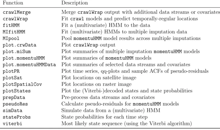
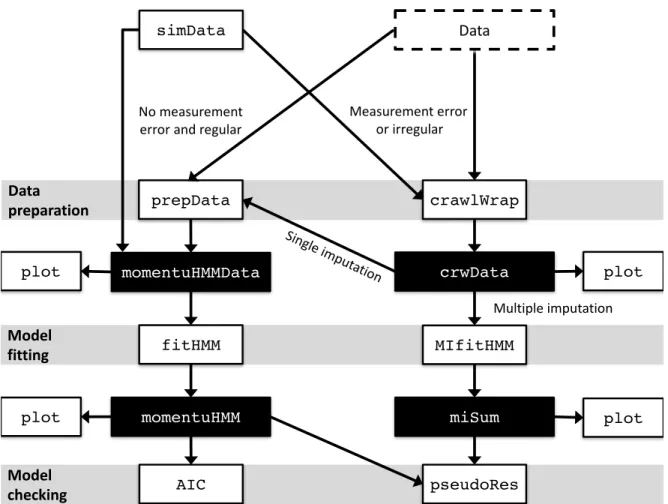
We first provide an overview of the main features and functions ofmomentuHMM. Step-by-step tutorials can be found in the package’s documentation (help(package="momentuHMM")) and vignette (vignette("momentuHMM")). The workflow formomentuHMM analyses con-sists of several steps (Fig. 1). These include data preparation, data visualization, model specification and fitting, results visualization, and model checking. The workhorse functions of the package are listed in Table 1. Usage of several of these functions is deliberately very similar to equivalent functions inmoveHMM (Michelotet al. 2016), but
the momentuHMM arguments for these functions have been generalized and expanded to
accommodate a more flexible framework for data pre-processing, model specification, parameterization, visualization, and simulation. R users already familiar withmoveHMM
will therefore likely find it easy to immediately begin using momentuHMM.
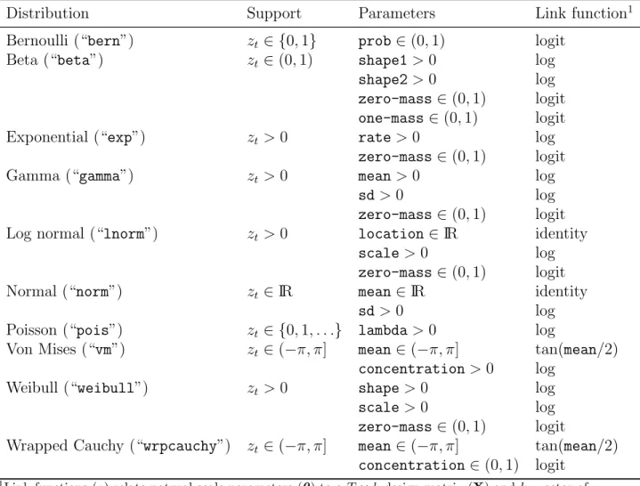
One of the key features of momentuHMMis the ability to specify an unlimited number of HMM data streams (e.g. step length, turning angle, altitude, heart rate) from a broad range of commonly used probability distributions (e.g. beta, gamma, normal, Poisson, von Mises). Using linear model formulas familiar to most R users, any of the data stream probability distribution parameters can be modelled as a function of environmental and individual covariates via link functions (Table 2). The state transition probabilities can also be modelled as a function of covariates using a multinomial logit link (e.g. Michelot
et al.2016). Permissable R classes for covariates includenumeric,integer, orfactor.
Spatio-temporal covariates (e.g. wind velocity, forest cover, sea ice concentration) can also beraster classes (Hijmans 2016), in which case the appropriate covariate values are automatically extracted based on the time and location of each observation (see section 3.3).
2.1
Data preparation and visualization
For temporally-regular location data with negligible measurement error, the prepData
function is used to create amomentuHMMDataobject that can be used for data visualiza-tion and further analysis. Summary plots of the momentuHMMData object returned by
func-tion. If location data are temporally-irregular or subject to measurement error, then a 2-stage multiple imputation approach can be performed (McClintock 2017). We discuss this pragmatic approach to incorporating uncertainty attributable to observation error and temporal irreglarity into multivariate HMM analyses in section 2.3.
2.2
HMM specification and fitting
Once a momentuHMMData object has been created using prepData, then the data are ready to be passed to the generalized multivariate HMM-fitting functionfitHMM. There are many different options for specifying HMMs usingfitHMM, so here we will only focus on several of the most important and useful features. The bare essentials of fitHMM
include the arguments:
• data A momentuHMMData object
• nbStates Number of latent states (N)
• dist A named list indicating the probability distributions of the data streams
• estAngleMeanA named list indicating whether or not to estimate the angle mean
for data streams with angular distributions (e.g. turning angle)
• formula Linear model formula for state transition probabilities
• stationaryLogical indicating whether or not the initial distribution is considered
equal to the stationary distribution
• Par0 A named list containing vectors of starting values for the state-dependent probability distribution parameters of each data stream
These seven arguments are all that are needed in order to fit the HMMs currently supported inmoveHMM(Michelot et al.2016), but the similarities between the packages largely end here. Many of the arguments in fitHMM and other momentuHMM functions are lists, with each element of the list corresponding to a data stream. Additional data streams can be added to HMMs by simply adding additional elements to these list arguments (see example in section 3.2).
The formulaargument can include many of the functions and operators commonly
formula argument can also be used to specify transition probability matrix models that incorporate cyclical patterns using the cosinor function (see example in section 3.1), splines for explaining other more complicated patterns (e.g.bsandnsfunctions in the R base packagesplines), and factor variables (e.g.formula=~IDfor individual-level effects). By default the formulaargument applies to all state transition probabilities, but special functions allow for state- and parameter-specific formulas to be specified (see example in section 3.4). Specific state transition probabilities can also be fixed to zero (or any other value), which can be useful for incorporating more behavioral realism by prohibiting or enforcing switching from one particular state to another (possibly as a function of spatio-temporal covariates).
Similar to the formula argument for state transition probability modelling, it is through the DM argument of fitHMM that covariate models are specified for the state-dependent probability distribution parameters for each data stream. DM formulas are just as flexible as theformulaargument and, in addition to common linear model for-mula functions and operators, can also include cyclical cosinor models, splines, factor variables, and state-specific probability distribution parameter formulas (see examples in sections 3.1, 3.3, and 3.4). Probability distribution parameters can also be fixed to user-specified values. However, specification of design matrices for probability distri-bution parameters using DM is not limited to formulas. Alternatively, “pseudo-design” matrices can be specified using an R matrix with rows corresponding to the natural parameters and columns corresponding to the working parameters. Pseudo-design ma-trices can be particularly useful for preventing state label switching when using multiple imputation methods (see section 2.3).
Another noteworthyfitHMM argument,circularAngleMean, enables users to spec-ify circular-circular regression models for the mean (µ) parameter of angular distribu-tions, such as the wrapped Cauchy and von Mises, instead of circular-linear models based on the tangent link function (Table 2). When circularAngleMean is specified for any given angular data stream (e.g. turning angle), then a special link function based on Duchesneet al. (2015) is used:
µ= atan2(sin(Xµ)βµ,1 + cos(Xµ)βµ), (2)
and the bearing of movement during the previous time step, i.e., each element
xt,i = atan2(sin(rt,i−bt−1),cos(rt,i−bt−1)) (3)
for angular covariate rt,i and i = 1, . . . , k. Because this link function is designed for
turning angles, a turning angle of 0 is provided as the reference angle. Thus as a trade-off between biased and correlated movements, the working parameters (βµ) for the expected turning angle at time t weight the attractive (or repulsive) strengths of the angular covariates relative to directional persistence. When all βµ = 0, the model reduces to a correlated random walk, but an increasingly biased random walk results as βµ gets larger (in absolute value). Many interesting hypotheses can be addressed using circular-circular regression, including the effects of wind, sea surface currents, and centers of attraction (or repulsion) on animal movement direction (see examples in section 3.3 and 3.4).
2.3
Multiple imputation
When location data are temporally-irregular or subject to measurement error, then they are not suitable for standard maximum-likelihood HMM analyses based on the forward algorithm (Eq. 1). In this case, momentuHMM can be used to perform the 2-stage multiple imputation approach of McClintock (2017). The basic concept is to first employ a single-state (i.e. N = 1) movement model that is relatively easy to fit but can accommodate location measurement error and temporally-irregular or missing observations (e.g. Johnsonet al.2008). The second stage involves repeatedly fitting the desired HMM tom temporally-regular realizations of the position process drawn from the model output of the first stage. Data streams or covariates that are dependent on location (e.g. step length, turning angle, habitat type, snow depth, sea surface temperature) will of course vary among them realizations of the position process, and the pooled inferences across the HMM analyses therefore reflect location uncertainty.
There are three primary functions (crawlWrap, MIfitHMM, and MIpool) for per-forming multiple imputation HMM analyses in momentuHMM, and all rely on parallel processing to speed up computations. Based on the R package crawl (Johnson 2017),
crawlWrapis a wrapper function for fitting the continuous-time correlated random walk
(CTCRW) model of Johnsonet al.(2008) and then predicting temporally-regular tracks of the user’s choosing (e.g. 15 min, hourly, daily). MIfitHMM is essentially a wrapper
function for fitHMM that repeatedly fits the same user-specified HMM to m imputed data sets. Based on them model fits, theMIpool function calculates pooled estimates, standard errors, and confidence intervals using standard multiple imputation formulae. See sections 3.2, 3.3, and 3.4 for example HMM analyses using multiple imputation to account for location measurement error and temporal irregularity.
2.4
Model visualization and diagnostics
The generic plot function for momentuHMM models plots the data stream histograms along with their corresponding estimated probability distributions, the estimated natu-ral parameters and state transition probabilities as a function of any covariates included in the model, and the tracks of all individuals (color-coded by the most likely state sequence). Confidence intervals for the natural parameters and state transition proba-bilities can also be plotted. For multiple imputation analyses, estimated 95% location error ellipses can be included in plots of individual tracks. The functions plotSat,
plotSpatialCov, and plotStates (Table 1) provide further methods for visualizing
model results. Diagnostic tools include the calculation and plotting of pseudo-residuals (Zucchini et al. 2016) using the pseudoRes and plotPR functions, respectively. For discrete distributions (e.g. Bernoulli, Poisson), a continuity adjustment is used for cal-culating pseudo-residuals. Akaike’s Information Criterion can be calculated for one or more models using the AIC.momentuHMM function.
2.5
Simulation
The function simData can be used to simulate multivariate HMMs from scratch or from an existing momentuHMM model. The arguments are very similar to those used for data preparation and model specification, but they include additonal arguments for simulating location data subject to temporal irregularity and measurement error. Among other features, rasters of spatio-temporal covariates and activity centers can be utilized (see section 3.4). simDatacan therefore simulate more ecologically-realistic tracks (potentially subject to observation error) for study design and power analyses. Goodness-of-fit can also be investigated by drawing simulated data sets from a fitted model and comparing them to observed properties of the data (Morales et al. 2004).
3
Examples
We will now demonstrate some of the capabilities of momentuHMM using real telemetry data. These examples are intended for demonstration purposes only, and we do not claim these example analyses represent improvements relative to previous or alternative analyses for these data sets. While space limits us to only a few key elements here, complete details and code for reproducing all examples described herein are provided in themomentuHMM “vignettes” source directory.
3.1
African elephant
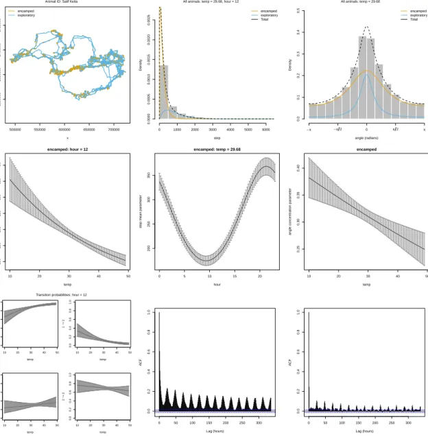
As our first example, we use an African elephant (Loxodonta africana) bull track de-scribed in Wallet al.(2014). In addition to hourly locations, the tag collected external temperature data. Location measurement error is negligible for these terrestrial GPS data, although about 1% of the hourly observations collected between 22 March 2008 and 30 September 2010 are missing. Instead of simply ignoring these missing data, we employed crawlWrap to predict the missing hourly locations prior to fitting a 2-state HMM assuming a wrapped Cauchy distribution for turning angle and a gamma distri-bution for step length. Autocorrelation function estimates suggest there are 24 h cycles in the step length data (Fig. 2), and this presents an opportunity to demonstrate the cosinor model for incorporating cyclical behavior in model parameters. We therefore included temperature effects on the turning angle concentration parameters and cycling temperature effects (with a 24 h periodicity) on the step length and state transition probability parameters.
When fitted usingfitHMM, this model identifed a state of slow undirected movement (“encamped”), and a state of faster and more directed movement (“exploratory”) (Fig. 2). About 74% of the steps were attributed to the “encamped” state, and 26% were at-tributed to the “exploratory” state. Interestingly, this model suggests step lengths and directional persistence for the “encamped” state decreased as temperature increased, step lengths for both states tended to decrease in the late evening and early morn-ing, and transition probabilities from the “encamped” to “exploratory” state decreased as temperature increased (Fig. 2). This model was overwhelmingly supported by AIC when compared to alternative models with fewer covariates, but model fit can be further assessed using pseudo-residuals. In this case, the pseudo-residuals indicate the model
explained much of the periodicity in step length, although there does still appear to be some room for improvement (Fig. 2).
3.2
Northern fur seal
We use the northern fur seal (Callorhinus ursinus) example from McClintock et al.
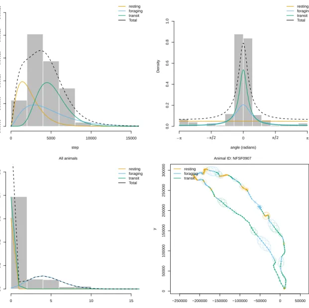
(2014) to demonstrate the use of additional data streams for distinguishing behaviors with similar horizontal trajectories (e.g. “resting” and “foraging”) in a multivariate HMM. The data consist of 241 temporally-irregular Fastloc GPS locations obtained during a foraging trip of a nursing female near the Pribilof Islands of Alaska, USA. The tag included time-depth recording capabilities, and the dive activity data were summarized as the number of foraging dives over T = 228 temporally-regular 1 h time steps. To fit the N = 3 state (1=“resting”, 2=“foraging”, 3=“transit”) model of McClintock et al. (2014) using momentuHMM, we first used crawlWrap to predict temporally-regular locations at 1 h time steps assuming a bivariate normal location measurement error model. We then used multiple imputation to account for location measurement error by repeatedly fitting the 3-state HMM to m = 100 realizations of the position process using MIfitHMM.
We specified a gamma distribution for step length, wrapped Cauchy distribution for turning angle, and Poisson distribution for the number of foraging dives. We used several arguments in MIfitHMM to avoid label switching among the 100 imputed data model fits and enforce similar state-dependent probability distribution constraints as McClintock et al. (2014), e.g. constraining the Poisson rate parameters such that the “foraging” state tends to have higher numbers of foraging dives than the “transit” state (λ2 > λ3).
Our results usingmomentuHMMwere very similar to those of the discrete-time Bayesian model of McClintock et al. (2014), with periods of “foraging” often followed by “rest-ing” at sea (Fig. 3). Activity budgets based on the estimated state sequences for each imputation were 0.3 (95% CI: 0.22−0.39) for “resting”, 0.29 (95% CI: 0.22−0.36) for “foraging”, and 0.41 (95% CI: 0.32−0.52) for “transit”.
3.3
Loggerhead turtle
Using hitherto unpublished loggerhead turtle (Caretta caretta) data for a captive-raised juvenile released on the coast of North Carolina, USA, we will now demonstrate how
movement direction and step length can be easily modelled as a function of angular covariates inmomentuHMM. The data consist of 165 temporally-irregular Argos locations and rasters of daily ocean surface currents collected between 20 November and 19 December 2012. Assuming a gamma distribution for step length (lt) and a wrapped Cauchy distribution for turning angle (φt), we modelled the mean step length parameter
(µl
t) as a function of ocean surface current speed (wt) and direction (rt) relative to the
bearing of movement (bt):
µlt = exp(β0l +β1lwtcos(bt−rt)), (4)
and the turning angle mean parameter (µφt) as a trade-off between short-term directional persistence and bias in the direction of ocean surface currents using the circular-circular regression link function:
µφt = atan2(sin(dt)βφ,1 + cos(dt)βφ), (5)
wheredt = atan2(sin(rt−bt−1),cos(rt−bt−1)).
We fit a 2-state HMM to the turtle data, with a “foraging” state unaffected by currents and a “transit” state potentially influenced by ocean surface currents as in Eqs. 4 and 5. We first usedcrawlWrapto predictT = 350 temporally-regular locations at 2 h time steps assuming a bivariate normal measurement error model that accounts for the Argos location quality class of each observation. We then again used multiple imputation to account for location uncertainty by repeatedly fitting the HMM tom = 100 realizations of the position process usingMIfitHMM. After preparing the data, this rather complicated HMM can be specified, fitted, and visualized in only a few lines of code:
nbStates <- 2
dist <- list(step = "gamma", angle = "wrpcauchy")
DM <- list(step = list(mean = ~state2(w:angle_osc), sd = ~1),
angle = list(mean = ~state2(d), concentration= ~1))
turtleFits <- MIfitHMM(miData, nbStates = nbStates, dist = dist,
Par0 = Par0, DM = DM,
estAngleMean = list(angle = TRUE),
circularAngleMean = list(angle = TRUE))
Note that thestate2special function inDMindicates the covariate formulas are specific to state 2 (“transit”), angle osc = cos(bt−rt), and the circularAngleMean argument
indicates that circular-circular regression link function is to be used on the mean turn-ing angle parameter as in Eq. 5. Complete details of the syntax above and code for reproducing this example can be found in the package vignette and supporting materi-als.
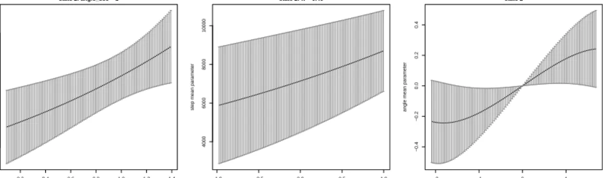
For the “transit” state, pooled parameter estimates indicated step lengths increased with ocean surface current speed and as the bearing of movement aligned with ocean surface current direction (βl
1 = 0.43,95% CI: 0.1−0.77; Fig. 4). The estimated wrapped
Cauchy distribution for turning angle had mean angles (µφt) biased towards the direction of ocean surface currents for each time step (βφ = 0.24,95% CI: −0.01−0.5), with concentration parameterρφ2 = 0.85 (95% CI: 0.77−0.92) indicating turning angles were concentrated at µφt. Thus movement during the “transit” state appears to strongly follow ocean surface currents (mean angle osc = 0.87,SD = 0.23), while movement during the “foraging” state exhibited shorter step lengths (µl
1 = 2996m,95% CI: 1791−
4202) perpendicular to ocean surface currents (mean angle osc = 0.07,SD = 0.26), with no directional persistence (ρφ1 = 0.03). The turtle spent 0.53 (95% CI: 0.34−0.71) of the 2 h time steps in the “foraging” state and 0.47 (95% CI: 0.29−0.66) of time steps in the “transit” state as it travelled northeast along a predominant current until it (presumably) found an attractive foraging patch (Fig. 4).
3.4
Grey seal
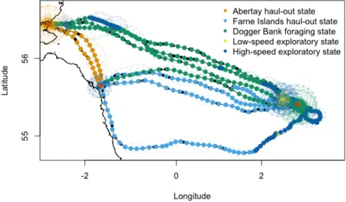
We now revisit an analysis of a grey seal (Halichoerus grypus) track that was originally conducted by McClintock et al. (2012) using Bayesian methods and computationally-intensive Markov chain Monte Carlo. The data consist of 1045 temporally-irregular Fastloc GPS locations collected in the North Sea between 9 April and 11 August 2008. Because the seal repeatedly visited the same haulout and foraging locations, it provides an excellent example for demonstrating how biased movements relative to activity cen-ters can be modelled usingmomentuHMM. McClintock et al.(2012) fitted a 5-state HMM to these data that included three “center of attraction” states, with movement bi-ased towards two haulout sites (“Abertay” and “Farne Islands”) and a foraging area (“Dogger Bank”), and two “exploratory” states (”low speed”, ”high speed”) that were unassociated with an activity center. After using crawlWrap to predict T = 1515
temporally-regular locations at 2 h time steps, we performed a very similar analysis to McClintock et al. (2012) using MIfitHMM by modeling the movement and transi-tion probability parameters as a functransi-tion of distance and angle to activity centers in a fashion similar to section 3.3. See the package vignette for further details and code.
Estimated activity budgets for the 5 states of this multiple-imputation HMM were 0.28 (0.27−0.3) for the “Abertay” haul-out state, 0.12 (0.11−0.14) for the “Farne Islands” haul-out state, 0.37 (0.35−0.38) for the “Dogger Bank” foraging state, 0.09 (0.03−0.2) for a low-speed “exploratory” state, and 0.14 (0.08−0.23) for a high-speed “exploratory” state. All three activity center states exhibited shorter step lengths and less biased movements when within the viscinity of these targets. Results from this analysis were thus very similar to those of McClintock et al. (2012), but this imple-mentation required far less computation time and no custom model-fitting algorithms. A simulated track generated usingsimData is presented along with the fitted track in Fig. 5.
4
Discussion
We have introduced the R package momentuHMM and demonstrated some of its ca-pabilities for conducting multivariate HMM analyses with animal location, auxiliary biotelemetry, and environmental data. The package allows for fitting and simulating from a suite of biased and correlated random walk movement process models (e.g. Mc-Clintocket al.2012). It can be used for an unlimited number of data streams and latent behavior states, includes multiple imputation methods to account for observation error and missing data, and integrates seamlessly with rasters to facilitate spatio-temporal covariate modelling. There are many types of analyses that can be conducted with
momentuHMM that hitherto required custom code and model-fitting algorithms,
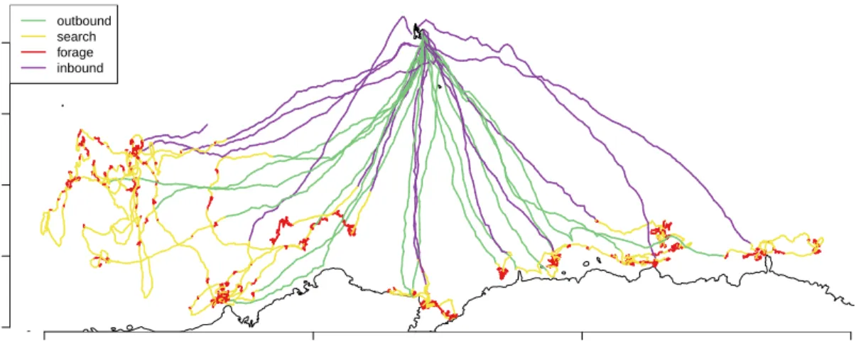
includ-ing the 3-state harbour seal model of McClintock et al. (2013), the 4-state southern elephant seal model of Michelot et al. (2017) (Fig. 6), the 6-state bearded seal model of McClintock et al. (2017), and the group dynamic model of Langrock et al. (2014). The package therefore greatly expands on available software and facilitates the incor-poration of more ecological and behavioral realism for hypothesis-driven analyses of animal movement that account for many of the challenges commonly associated with telemetry data. While many of the features of momentuHMM were motivated by animal
movement data, we note that the package can be used for analyzing any type of data that is amenable to HMMs.
Model fitting in momentuHMM is relatively fast because the forward algorithm (Eq. 1) is coded in C++. Because multiple imputations are completely parallelizable, with sufficient processing power computation times for analyses that account for measure-ment error, temporal irregularity, or other forms of missing data need not be longer than that required to fit a single HMM. However, computation times will necessarily be longer as the number of states and/or parameters increase. For example, momentuHMM
required about 1 hour to fit a single HMM withN = 6 states, seven data streams, and
T = 7414 time steps (McClintock 2017) on a standard desktop computer.
As in any maximum likelihood analysis based on numerical optimization, compu-tation times will also depend on starting values. Specifying “good” starting values is arguably the most challenging aspect of model fitting, and the package includes several functions that are designed to help with the specification of starting values. It also includes options for re-optimization based on random perturbations of the parameters to help explore the likelihood surface and diagnose convergence to local maxima.
WhilemomentuHMMincludes functions for drawing realizations of the position process based on the CTCRW model of Johnsonet al.(2008), this is but one of many methods for performing the first stage of multiple imputation. Realizations of the position pro-cess from any movement model that accounts for measurement error and/or temporal irregularity (e.g. Calabrese et al. 2016) could be passed to MIfitHMM for HMM-type analyses in the second stage. Multiple imputation methods also need not be limited to these telemetry error scenarios. For example, other forms of missing data could be im-puted, thereby allowing investigation of non-random mechanisms for missingness that can be problematic if left unaccounted for in HMMs.
There remain many potential avenues for refinement and extension. Computation times could likely be improved by further optimizing the code for speed. Notable extensions include hidden semi-Markov models and random effects (Zucchini et al.
2016). It is straightforward to add additional data stream probability distributions, and practitioners interested in additional features are encouraged to contact the authors.
Acknowledgments
We are grateful to R. Scott, B. Godley, M. Godfrey, J. Sudre, and North Carolina Aquariums for providing the data used in our turtle example. The findings and con-clusions in the manuscript are those of the author(s) and do not necessarily represent the views of the National Marine Fisheries Service, NOAA. Any use of trade, product, or firm names does not imply an endorsement by the US Government.
References
Beyer, H.L., Morales, J.M., Murray, D. & Fortin, M.J. (2013) The effectiveness of Bayesian state-space models for estimating behavioural states from movement paths.
Methods in Ecology and Evolution, 4, 433–441.
Calabrese, J.M., Fleming, C.H. & Gurarie, E. (2016) ctmm: an R package for analyzing animal relocation data as a continuous-time stochastic process. Methods in Ecology
and Evolution, 7, 1124–1132.
Costa, D.P., Robinson, P.W., Arnould, J.P., Harrison, A.L., Simmons, S.E., Hassrick, J.L., Hoskins, A.J., Kirkman, S.P., Oosthuizen, H., Villegas-Amtmann, S. et al.
(2010) Accuracy of argos locations of pinnipeds at-sea estimated using fastloc gps.
PloS one,5, e8677.
DeRuiter, S.L., Langrock, R., Skirbutas, T., Goldbogen, J.A., Chalambokidis, J., Fried-laender, A.S. & Southall, B.L. (2017) A multivariate mixed hidden Markov model to analyze blue whale diving behaviour during controlled sound exposures. The Annals
of Applied Statistics, 11, 362–392.
Duchesne, T., Fortin, D. & Rivest, L.P. (2015) Equivalence between step selection func-tions and biased correlated random walks for statistical inference on animal move-ment. PLoS ONE, 10, e0122947.
Hijmans, R.J. (2016)raster: Geographic Data Analysis and Modeling. R package version 2.5-8.
Johnson, D.S. (2017)crawl: Fit Continuous-Time Correlated Random Walk Models to
Johnson, D.S., London, J.M., Lea, M.A. & Durban, J.W. (2008) Continuous-time cor-related random walk model for animal telemetry data. Ecology, 89, 1208–1215.
Jonsen, I.D., Flemming, J.M. & Myers, R.A. (2005) Robust state–space modeling of animal movement data. Ecology,86, 2874–2880.
Langrock, R., Hopcraft, G., Blackwell, P., Goodall, V., King, R., Niu, M., Patterson, T., Pedersen, M., Skarin, A. & Schick, R. (2014) Modelling group dynamic animal movement. Methods in Ecology and Evolution, 5, 190–199.
Langrock, R., King, R., Matthiopoulos, J., Thomas, L., Fortin, D. & Morales, J.M. (2012) Flexible and practical modeling of animal telemetry data: hidden markov models and extensions. Ecology, 93, 2336–2342.
McClintock, B.T. (2017) Incorporating telemetry error into hidden markov models of animal movement using multiple imputation. Journal of Agricultural, Biological, and
Environmental Statistics, 22, 249–269.
McClintock, B.T., Johnson, D.S., Hooten, M.B., Ver Hoef, J.M. & Morales, J.M. (2014) When to be discrete: the importance of time formulation in understanding animal movement. Movement Ecology, 2, 21.
McClintock, B.T., King, R., Thomas, L., Matthiopoulos, J., McConnell, B.J. & Morales, J.M. (2012) A general discrete-time modeling framework for animal move-ment using multistate random walks. Ecological Monographs, 82, 335–349.
McClintock, B.T., London, J.M., Cameron, M.F. & Boveng, P.L. (2017) Bridging the gaps in animal movement: hidden behaviors and ecological relationships revealed by integrated data streams. Ecosphere,8, e01751.
McClintock, B.T., Russell, D.J., Matthiopoulos, J. & King, R. (2013) Combining indi-vidual animal movement and ancillary biotelemetry data to investigate population-level activity budgets. Ecology, 94, 838–849.
Michelot, T., Langrock, R., Bestley, S., Jonsen, I.D., Photopoulou, T. & Patterson, T.A. (2017) Estimation and simulation of foraging trips in land-based marine predators.
Michelot, T., Langrock, R. & Patterson, T.A. (2016) moveHMM: An R package for the statistical modelling of animal movement data using hidden markov models. Methods
in Ecology and Evolution, 7, 1308–1315.
Morales, J.M., Haydon, D.T., Frair, J., Holsinger, K.E. & Fryxell, J.M. (2004) Extract-ing more out of relocation data: buildExtract-ing movement models as mixtures of random walks. Ecology, 85, 2436–2445.
R Core Team (2017) R: A Language and Environment for Statistical Computing. R Foundation for Statistical Computing, Vienna, Austria.
Wall, J., Wittemyer, G., LeMay, V., Douglas-Hamilton, I. & Klinkenberg, B. (2014) Elliptical time-density model to estimate wildlife utilization distributions. Methods
in Ecology and Evolution, 5, 780–790.
Whoriskey, K., Auger-M´eth´e, M., Albertsen, C.M., Whoriskey, F.G., Binder, T.R., Krueger, C.C. & Mills Flemming, J. (2017) A hidden markov movement model for rapidly identifying behavioral states from animal tracks. Ecology and Evolution, 7, 2112–2121.
Zucchini, W., MacDonald, I.L. & Langrock, R. (2016)Hidden Markov Models for Time
Table 1. Workhorse functions for the R package momentuHMM.
Function Description
crawlMerge Merge crawlWrap output with additional data streams or covariates
crawlWrap Fit crawl models and predict temporally-regular locations
fitHMM Fit a (multivariate) HMM to the data
MIfitHMM Fit (multivariate) HMMs to multiple imputation data
MIpool Pool momentuHMM model results across multiple imputations
plot.crwData Plot crawlWrap output
plot.miSum Plot summaries of multiple imputation momentuHMM models
plot.momentuHMM Plot summaries of momentuHMM models
plot.momentuHMMData Plot summaries of selected data streams and covariates
plotPR Plot time series, qq-plots and sample ACFs of pseudo-residuals
plotSat Plot locations on satellite image
plotSpatialCov Plot locations on raster image
plotStates Plot the (Viterbi-)decoded states and state probabilities
prepData Pre-process data streams and covariates
pseudoRes Calculate pseudo-residuals for momentuHMM models
simData Simulate data from a (multivariate) HMM
stateProbs State probabilities for each time step
Table 2. Data stream (z) probability distributions, natural parameters, and default link functions for covariate modelling. Probability distributions with positive support can be zero-inflated (with additional zero-mass parameters), while the beta distribution can be zero- and one-inflated (with additional one-mass parameters). If user-specified bounds are provided, then custom link functions are used instead of the defaults (see momentuHMM package doc-umentation for further details). If circular-circular regression is specified for the mean of angular distributions (“vm” and “wrpcauchy”), then a link function based on Duchesneet al. (2015) is used. Users seeking additional data stream probability distributions are encouraged to contact the authors.
Distribution Support Parameters Link function1
Bernoulli (“bern”) zt ∈ {0,1} prob∈(0,1) logit
Beta (“beta”) zt ∈(0,1) shape1 >0 log
shape2 >0 log
zero-mass∈(0,1) logit
one-mass∈(0,1) logit
Exponential (“exp”) zt >0 rate>0 log
zero-mass∈(0,1) logit
Gamma (“gamma”) zt >0 mean>0 log
sd >0 log
zero-mass∈(0,1) logit
Log normal (“lnorm”) zt >0 location∈IR identity
scale >0 log
zero-mass∈(0,1) logit
Normal (“norm”) zt ∈IR mean∈IR identity
sd >0 log
Poisson (“pois”) zt ∈ {0,1, . . .} lambda >0 log
Von Mises (“vm”) zt ∈(−π, π] mean∈(−π, π] tan(mean/2)
concentration>0 log
Weibull (“weibull”) zt >0 shape >0 log
scale >0 log
zero-mass∈(0,1) logit
Wrapped Cauchy (“wrpcauchy”) zt ∈(−π, π] mean∈(−π, π] tan(mean/2)
concentration∈(0,1) logit
1Link functions (g) relate natural scale parameters (θ) to a T×kdesign matrix (X) andk−vector of
Model checking Model fitting Data preparation prepData plot momentuHMMData crawlWrap No measurement
error and regular Measurement erroror irregular
fitHMM plot momentuHMM crwData MIfitHMM AIC plot miSum plot pseudoRes Multiple imputation Data simData
Figure 1. Schematic representing the typical momentuHMM workflow. White boxes indicate package functions and black boxes indicate object classes returned by functions. When teleme-try data are subject to location measurement error or temporal irregularity, these sources of uncertainty can be incorporated into HMMs using single or multiple imputation of the position process via the crawlWrap function.