Growth and poverty in rural India

POLICY RESEARCH WORKING

PAPER

1405

.'~ g tur

Growth and Poverty

Higheragcul

es

-reduced absolute poverty-in

in Rural India

smaliholder productivi and

Marti

Ravary

Martin Ravallion

-;

.

G a Da

Gaurav Datt

i.--

were far smaller in the short: run-than in the iong run..

Badcground paper for

World

Daveopment

Report

1995S

The World

Bank

Office of

the Vice

Preident

-Deve[opment Economic A

-January

1995

Public Disclosure Authorized

Public Disclosure Authorized

Public Disclosure Authorized

POLICY RI!SeARCH WORKING PAPER 1405

Summary findings

Unlike most developing countries, consistent poverty yields, which benefited poor people both directly and measures for India can be tracked over a long time. through highcr rcal agricultural wages. And thc benefits Ravallion and Datt used 20 houschold surveys for rural from higher yiclds were not confined to those near the India for the years 1958-90 to measure the effects of poverty line - the poorest also benefited.

agricultuml growth on rural poverty and on the rural The process through which India's rural poor labor market and to find out how long it takes for the participate in the gains from agricultural growth takes

effects to be felt. time, although about half of the long-run impact comes

They found that mcasures of absolute rural poverty within three years.

responded elastically to changes in mean consumption. The long-run elasticity of the head-count index to farm But agricultural growth had no discernible impact - yield was over 2 - of which 40 percent came through

either positive or negative - on the share of total wages. Short-run elasticities were far smaller.

consumption going to the poor. Inflation adversely affected the rural poor by eroding For the rural poor, Ravallion and Datt artribute the their real wages in the short run.

long-run gains from growth to higher average farm

This paper - a product of the Office of the Vice President, Development Economics - is one in a series of background papexs prepared for WorldDevelopment Report 1995 en labor. Copies of the paperare available free from the World Bank, 1818 H Street NW, Washington, DC 20433. The study was funded by the Baaik's Research Support Budget under the research project "Poverty in India, 1950-90" (RPO 677-82). Plcase contact the World Development Report office, room T7-101, cxtension 31393 (34 pages). January 1995.

The Policy Researcb Workixg Paper Series disseminates the findings of work sn prOgress to encourage the exchange of ideas about

development isswes An objective of thesries s toget the fiings outquickly. cven if thc presentaionsare less than fdly polished The

papers cany the names of the authorsand should be usedandciftdaccordingly. The findings, interpretations, and conclusions are the

Growth and Poverty in Rural India

Martin Ravallion and Gaurav Daet

Policy Research Department, World Bank, 1818 H Street NW, Washington DC. These are the views of the authors, and should not be attributed to the World Bank. The support of the Bank's

Research Committee (under RPO 677-82) is gratefully acknowledged. The authors are also grateful to Berk Ozler for help in setting up the data set used here. The comments of James Boyce. Lyn Squire, Dominique van de WaUe, Michael Walton, and seminar participants at Cornell University, the International Food Policy Research Institute and the World Bank are gratefully acknowledged.

1 Introduction

The scope for economic growth to make a real difference in the lives of the developing world's poor has been the subject of (often vociferous) debates in both academic and policy circles.' Measuring the long-rm benefits to poor people from economy-wide changes calls for a time series of representative household-level surveys; yet such surveys are sporadic at best for most countries. India is an exception. There one can trace distributional impacts o ier a long period using reasonably comparable and nationally representative surveys of consumption.2

Here we use these surveys to examine how much India's rural poor have benefited from agricultural growth, what role the labor market has played, and whether the impacts were distributionally biased one way or another. We depart from past analyses for India and elsewhere in five main ways:

i) The identification of distributional impacts. It is theoretically possible for a growth process to have sufficiently adverse effects on inequality that poverty increases, and some have argued that this is also the reality of India's rural development. Another view-often termed

"trickle down"-denies this, but still allows that distribution may worsen even though on balance the poor gain somewhat. By contrast, some growth processes can entail favorable distnbutional

I Recent surveys spanning the wide range of views concerning the impacts of growth in farm productivity on rural poverty include Saith (1990), Singh (1990) and Lipton and Ravallion (1994). Differences between countries or time periods may account for some of these differences, but certainly not all. Contrast, for example, Ahluwalia's (1978, p.320) conclusion that "..there is evidence of some trickle down associated with agricultural growth" with Saith's (1981, p.205) claim that "there can be little doubt that current growth processes have served as generators of poverty"; both were using data for the same country (India) over roughly the same period (1957-73).

2 It seems that not even for the U.S.A. can one track poverty measures as well. The were 15 Consumer Expenditure Surveys for the U.S.A. over the same period for which we have 20 National Sample Surveys for India.

shifts, and consequently larger gains to the poor than a "trickde down'. Here we propose a method for identifying and testing the distributional impacts of growth on poverty.

ii) The role plaved by the labor market. Past work has often ignored or down-played the rural labor market's capacity to transmit the benefits of technical progress to the poor. Marked differences in emphasis can be found in policy-oriented discussions on this point.3 Here we aim

to quantify the role played by real wages in distributing the gains from aggregate growth. iii) Allowing for dynmic effects. The dynamics of the distributional impacts of growth are of obvious interest, though the topic has received surprisingly little attention. Past models have analyzed the consumption-based poverty measures within a static framework, despite theory and evidence to the contrary. Stickiness in the adjustment of poverty measures also has an important implication: long-run responses can far exceed those in the short-run.

iv) The time period of analsis. Much of the scholarly debate for India has focused (often-though not always-for lack of data) on periods of rather little growth; these data may have low power in testing the effects of growth on poverty (Srinivasan, 1985). We use a new data set embracing a period (since the mid-1970s) of higher agricultural growth.

v) The treatment of survey spacing. Unlike past work, we deal consistently with the uneven survey spacing in the estimation. This can matter to estimating dynamic effects.

The following section outlines the model we will be using. Section 3 then presents our results, while conclusions can be found in section 4. Appendix 1 describes our data and its sources, while Appendix 2 discusses related work in the literature on rural poverty in India.

I Contrast, for cxample, the IFAD (1992) report with World Bank (1990). The former emphasizes the scope for reducing rural poverty by developing smallholder agriculture, and pays little attention to the role of the unskilled labor market; by contrast the World Bank report emphasizes the importance of positive employment and wage effects in achieving pro-poor growth (though not to the exclusion of other channels).

2 Modelling bnpats of growth on poverty

2.1 Characterizing alternative growth processes

A poverty measure (P) can be written as a non-increasing function of the mean (p), and a vector of parameters $. = (x ,--,) for the Lorenz curve:4

P = P(P, a) (1)

Let the Lorenz parameters also vary with the mean 2L(p) (other variables are ignored for now) and consider the effect of an increase in the mean.' Assume that all these functions are

differentiable, and let subscripts denote partial derivatives. We can distinguish three cases:

i) Immis_rizin growth; dP/dp m = Pp + EP¶I-x1, > 0. This requires that 2P., is

4.'

sufficiently positive to outweigh the direct impact of growth (since P. : 0).

ii) "Trickle down"6; dP/dp < 0 but EP3nfF a 0. While the distribudonal shft do not

favor the poor. the growth effect is still strong enough that poverty falls. We call the special case in which EP.

:sp

iii) Redistribution widt grow Eh; nP,1 JCP< 0. Here the redistribution is also pro-poor.

4 The mean is taken to be normalized by the poverty line. For explicit formulae for these

relationships in the case of the poverty measures used here see Datt and Ravallion (1992).

s On the effects of a change in the mean on a poverty measure holding the Lorenz curve constant see Kakwani (1993). Here we allow the Lorenz curve to also vary.

' This term is sometimes used in any situation in which the poor share in economic gromwth. But if all the growth was from gains to poor people, this is surely not "trickle down", which suggests a limited gain to the poor from a growth process subsially involving nonpoor people.

How can one distinguish these cases empirically? While the rediscribution effects can be difficult to disentangle, we can readily determine the sign of EP, 7t, by constructing the

simU!ated poverty

measures:

Pe = pN, a(p) (2)

for fixed p but using the actual Lorenz curve; the poverty measures are thus purged of the direct

effect of growth, leaving only the effect via changes in the Lorenz curve. We then examine the relationship between P and p, so as to distinguish the three cases above (noting that

dP7di = 2P, xx). ₁ To estimate P' one multiplies all consumptions by p / p (thus preserving

the actual Lorenz curve) and then calculates the poverly measure on the scaled distribution. What is P'? It is not an inequality measure as such,7 but a measure of how inequality

matters to the poor. One can interpret P. as a measure of "relative poverty" in which the poverty line is set as a fixed proportion of the mean, as distinct from the 'absolute poverty measure" P(p,, z,). But P' does not have much appeal as a poverty measure in its own right

(since it is unaffected by distribution-neutral changes, even when tfiey entail substantial gains or losses to poor people); rather it is an analytic construct to help understand the distributional effects of growth. That is the way we will use it in the following analysis.

7 For some possible poverty measures, it will not satisfy the Pigou-Dalton transfer axiom. 8 For discussion and references on this distincton, and the properties of both types of

measures, see Ravallion (1994).

2.2 An econometric model

A time series of individual consumption is likely to be sticky, due to smoothing behavior. The poor are widely thought to be less well insured than others, yct it is also clear that they often self-insure (Alderman and Paxson, 1992; Deaton, 1992); the cost of not doing so can be

prohibitively high. While there is evidence against the Permanent Income Hypothesis in rural India (Bhargava and RavaUlion, 1993), consumption is clearly smoother than income (Walker and Ryan, 1990).

However, the way serial correlation in individual consumption is tralated into the dynamic behavior of a time series of poverty measures (based on cross-sections of consumption)

is likely to be complex.9 This will also depend on the covariances across individuals. Suppose that there is no smoothing behavior at the individual level, in that current consumption is simply current income, but that incomes are negatively correlated across individuals; those that escape poverty are replaced by others. Then one could find serial dependence in the poverty measures even though individual consumptions fluctuate wildly. While we are skeptical about the prospects of disentangling these sources of dynamics in aggregate poverty measures, one cannot rule out the possibility that fteir adjustment to changes in current variables is far from instantaneous. Thus the econometric specification must allow for dynamic effects.

The choice of poverty measures is also an issue. It has been argued that the bulk of gains amongst the poor go to those near the poverty line (Lipton, 1983). To test this, one needs

measures of poverty which better reflect its depth and severity than the popular "headcount index" given by the proportion of people deemed poor.

I We shall not go into the issue of whether poverty should be measured in terms of consumption or income, for we have no choice in this context since India's NSS does not include income. For further discussion of this issue from various perspectives see Atkdnson (1991), Slesnick (1993), and Ravallion (1994).

Combining these considerations, a simple test of whether the poor shared in growth is to regress the poverty measure against the mean of the distribution. On allowing for dynamnic effects we estimate:

InP₆ a I,aO + %,₁InP., + i

Wlf1pt

where P., is the Foster-Greer-Thorbecke (1984) measure for date t (described below), and p, is mean consumption at date t. A significant (negative) estimate of 7 .2 could reflect Lorenz curve

shifts either for or against the poor. So, in addition to (3), we estimate the regression:

IP,', 7 + I91jnP;t-1 + *421np + v(4)

where P., is the relative poverty measure (equation 2) obtained by re-estimating P., applying a fixed reference mean to the Lorenz curve for date t.

The poverty measures are formed by taking a (household-size weighted) mean of household-level poverty measures based on consumption-poverty gaps; specifically:

P.i=g

L1

in which xi is consumption expenditure per person in the i'th household of size s, in a population of n households, z is the poverty line, and a is a non-negative parameter which we allow to take three possible values: i) a=0, giving the headcount index: ii) a= 1, the poverty ga index and iii) a=2, the sguared povertv ggp index.'0 The headcount index is the most popular measure,

but-unlike the other two measures-it is unresponsive to changes below the poverty line.

10 nthe reasons for preferring additive measures to non-additive ones, such as the Sen (1976) index, see Foster and Shorrocks (1991).

Our principal concerns in estimating these various models for the poverty measures arise from two intrinsic limitations of our data: the first is that, after allowing for missing data, we have only 20 observations for the poverty regression, and the second is that those observations are unevenly spaced. Even if we achieve consistency, small sample biases in the tpes of models we are estimating will probably entail some underestimation of the true values of the 7cl S.l

We shall try two approaches for dealing with the irregularity of the household surveys. Let r, denote the elapsed time since the last survey. On eliminating terms in the unknown poverty measures between surveys, we can then re-write equation (3) as:

(6)

+ 2= (lnPI, + + -1 Ut

However, this is still not a readily estimable model; it requires the survey means for years between surveys and (in effect) it has a different number of variables in different observations (according to the variation in ;). The model becomes tractable if we re-write it as:

W 7Cz1XP-s (I -XT9s2lRf ) + d(7)

lnP,

:"h',bP.

1np

However, this does modify the properties of the error term, as it now inludes deviations of Inp, 1 from its value at time t for iss,l. If 1lnp,_ behaves as an autoregressive process during

the period since the last survey, the new error term will still be heteroscedastic (since the uneven

spacing will mean hat the error variance tends to be larger aftr longer gaps).'2 _{We shall later}

examine the properties of the model's residuals to see if this is a serious concern. Nonetheless, this specification is probably better than ignoring the gaps, or interpolating for the missing values.

A second approach can be suggested. If we start from a slightly different model by adding a term in 7t,3In.,-. tO the right hand side of (3) and

apply

lnPa=

1

t9 In,-+

(-')-

,, ,,ZS.t-,+, O(I ) .+.2(lflp, - Sallnmu,) (

This does not require data between surveys. Under the (here untestable) common factor

restrictiorns the new error term (,;,) is vat + iC£i + + tc' at-t,.1 The implicit coefficient

on llfi,-. is IC 3 ` - Sal 2J We shall also try

this

2.3

The above discussion has outlined a method of assessing how pro-poor the distributional effects of growth are. But how does agricultural growth in particular affect the mean and Lorenz parameters of the distribution of consumption?

As in most of Asia, the vast bulk of the rural poor in India are either landless or live on small farms with inadequate land for even their food needs. They depend heavily on earnings from supplying unskilled wage labor to other farm or non-farm enterprises. In principle there are

12 The new error term contains terms in lnp,-Inj, ,. With Inli, following an AR process, the

error term will still have a zero mean.

two channels thSough which they might benefit from economic growth. One is by participating directly in that growth by producing more on their own land; the other is through the labor market.

The new farming technologies that started to be adopted in India fron around 1970 allowed higher output by both raising yield per acre sown and by permitting multiple cropping of a given land area within one year. Of the two ways in which the landless rural poor might benefit from this growth-extra employment or higher wages-the latter channel is more

contentious; indeed, early development theories assumed a rural economy in labor surplus, such that extra employment would have no effect on the real wage (Lewis, 1954; Ranis and Fei,

1961). By this view, there would be little scope for trickle down via real wages.

However, other models of the rural labor market allow a labor surplus to coexist with a process of wage determination in which labor-augmnenting technical progress can lead to higher real wages. i3 The dynamics of such effects are also of concern here. Short-run stickiness is a

widely observed property of formal sector wages, but it has also been observed in rural settings in which there are no trade unions or binding minimum wage rates (Boyce and Ravallion, 1991). In poor rural economies employers will resist wage increases at least initially, and the cxistcncc of tacit collusion or other forms of resistance on the supply side in village labor markets could also yield short run stickiness downwards. Long-run responses of real wages to agricultural growth can thus exceed short-run responses.

Motivated by the above arguments, we would also like to test whether or not: i) rural poverty depends on both average real wages in agriculture and average farm productivity; ii) real

1" For a survey of various models of rural labor markets in this setting see Draze and Mukherjee (1989). Examples of the models we refer to include Osmani (1991) and Mukhedjee and Ray (1992).

wages are directly responsive to productivity; iii) both poverty and wages are positively serially dependent, in that (ceteris paribus) they will tend to be closer to their latest values than more distant ones; and iv) any pro-poor impact of higher farm productivity and wages persists after controlling for changes in mean consumption.

The economic model we have in mind for the long-run determinants of poverty gives individual consumption as a function of the real wage rate, a measure of technical progress in agriculture, other exogenious aggregate variables, and an unobserved idiosyncratic variable reflecting individual endowments. Integrating out the latter variable, the long run poverty measure defined on the distribution of consumption can be written as a fimution of the wage and the farm productivity variable. The long run wage we assume to also be a fimction of farm productivity, via (for example) a long run labor market clearing condition. The adjustment process toward these long run values is taken to be a simple autoregressive process, and we assume that the relationships of interest are linear in logarithms.

Thus we estimate the following triangular system:

-nPl =

Po

P

(9)

lnW, = yo + y lflW,_. + Y2?Xr + t

where W, is the real wage rate for agricultural labor at t,

X.

variables including average farm productivity, the P,3 's and y,'s are parameters to estimate, and

e,, v, are assumed to be normally distributed white noise error processes. Similarly to equation

(4) we shall then also re-estimate the model after replacing the poverty measurs by P,[r to test for distributional impacts on poverty. To deal with uneven spacing we will estimate nonlinear models analogous to equations (7) and (8).

3 Results

?.1 Data

We shall be using 20 rounds of India's National Sample Survey, spanning the period 1958-90. The gaps between surveys range from 11 months to 5.5 years. It is clearly less than ideal to be estimating a dynamic model from only 20 time series observations, and unevenly spaced as well. While more surveys are available (for the 1950s) other data (notably wages) are not. The distributions are of household consumption expenditure (including from own

production) per person. The poverty line is the official one for India, produced by the Panning Commission. For the relative poverty measures we use the overall mean as the reference (pi in equation (2)), equivalent to setting poverty lines at 84% of each date's mean. The wage data are for male agricultural wages.'4 _{The price deflator for both the poverty line and wages is the}

Consumer Price Index for Agricultural Laborers. We measure farm productivity by agricultural output per acre, output being measured by a value-weighted quantity index of production of all crops."5 Appendix 1 describes the data more fully, whie Appendix 2 describes the relationship

with other specifications found in the literature.

The basic time pattern of the evolution of rural poverty has been one of fluctuation without a trend up to about the mid-1970s and a significant decline thereafter (see Table A2 and Figures 2, 3 in Appendix 1). The contrast between the two periods, 1958-75 and 1975-90, is also borne out by the annual growth rates in Table 1. The latter 15-year period saw sigaificantly

14 A complete time series is not available for women.

" Alternatively one can use value added in agriculture, though this makes little difference since it is highly correlated with output (r=0.97 in logs).

Table 1; Annual growth rates of selected variables

Average annual rate of growth (%) 1958-75 1975-90

Head-count index 0.96 -3.87

Poverty gap index 1.09 -6.38

Squared poverty gap index 1.22 -8.15

Real mean per capita consumption -0.93 1.76

Real agricultural wage rate 0.06 3.36

Agricultural output per acre of net sown area (YNS) 1.58 2.89

Net sown area per person in rural areas (NSAPC) -1.57 -1.91

Agricultural output per person in rural areas (YPC) 0.00 0.97

higher rates of decline in all poverty measures alongside higher growtb rates for real mean per capita consumption, real agricultural wages and agricultural yield.

3.2 Regressions for the poverty measures as functions of the mean

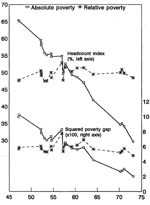
Figure 1 plots both the headcount index and squared poverty gap against mean consumption. We give both the absoiute poverty measures implied by the actual mean and

Lorenz curve for each date, as well as the relative poverty measures based on the actual Lorenz curve and a fixed reference mean so as to isolate the distributional effects (section 2.1). For the absolute poverty measures there is strong negative correlation with the mean. This vanishes for the relative poverty measures; there is no sign of distributional effects for or against the poor.

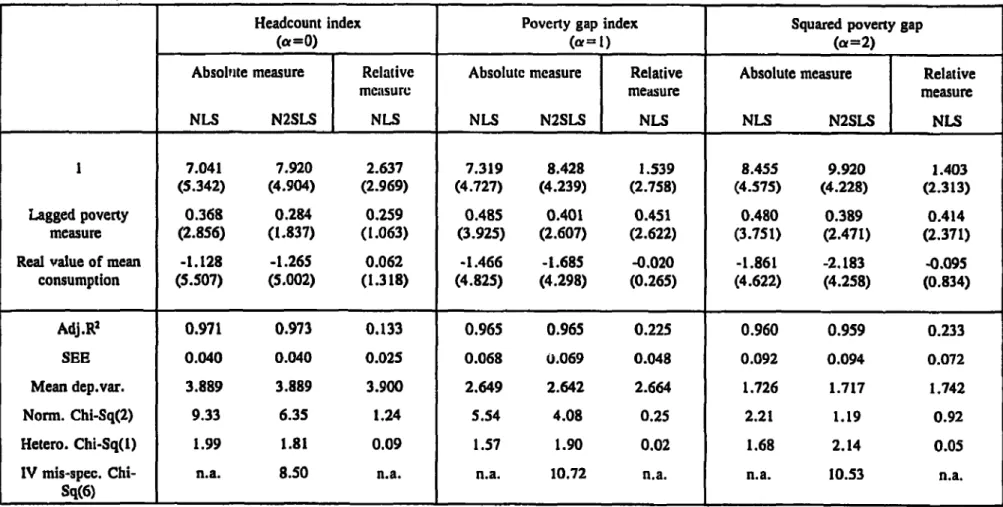
To estimate the poverty regressions against the mean in the form of equations (7) or (8) we used Amemiya's (1974) nonlinear least squares (NLS) and nonlinear two-stage least squares (N2SLS) methods, as programmed by Pesaran and Pesaran (1991). Our estimates of equations (3) and (4) are given in Table 2. For the N2SLS estimator the instrumental variables were the

lagged poverty measures, the lagged mean, lagged real wages, lagged yield per acre and a time trend. We subjected all these regressions to a battery of standard residual diagnostic ts,

including serial correlation (up to two years), normality, heteroscedasticity (squared residuals regressed against squared fitted values, though we also tried the length of time between surveys on its own), autoregressive heteroscedasticity (up to two years), and a miss-specification test for generalized IV estimation which can be interpreted as a test of exogeneity of instruments. All tests were passed comfortably.

The short-run elasticities to the mean vary from -1.1 to -2.2, being higher the higher the value of a. (We conmment further on that property later.) The positive autocorrelation in the three poverty measures entails higher long-run elasticities which range from -1.8 to -3.6 again

Figure 1: Poverty Measures

Against Mean

Consumption

70

Absolute poverty

Relative poverty

65

60

55

Headcount

index

( left axis)

50

-% ,b'

-45

1 2

40

1 0

35

Squared

poverty gap

8

(xl 00, right axis)

30A

6

4

2

l

I

I

I

I

0

45

50

55

60

65

70

75

Mean consumption (Rs/ps/mth,1973-74 prices)

Table 2: Poverty measures as functions of the mean

Headcount index Poverty gap index Squared poverty gap

(Ot=0) (of= 1) (of=2)

Absolute measure Relative Absolute measure Relative Absolute measure Relative

measure measure measure

NLS N2SLS NLS NLS N2SLS NLS NLS N2SLS NLS

1 7.041 7.920 2.637 7.319 8.428 1.539 8.455 9.920 1.403

(5.342) (4.904) (2.969) (4.727) (4.239) (2.758) (4.575) (4.228) (2.313)

Lagged poverty 0.368 0.284 0.259 0.485 0.401 0.451 0.480 0.389 0.414

measure (2.856) (1.837) (1.063) (3.925) (2.607) (2.622) (3.751) (2.471) (2.371) Real value of mean -1.128 -1.265 0.062 -1.466 -1.685 -0.020 -1.861 -2.183 -0.095

consumption (5.507) (5.002) (1.318) (4.825) (4.298) (0.265) (4.622) (4.258) (0.834) Adj.R2 0.971 0.973 0.133 0.965 0.965 0.225 0.960 0.959 0.233 SEE 0.040 0.040 0.025 0.068 0.069 0.048 0.092 0.094 0.072 Mean dep.var. 3.889 3.889 3.900 2.649 2.642 2.664 1.726 1.717 1.742 Norm. Chi-Sq(2) 9.33 6.35 1.24 5.54 4.08 0.25 2.21 1.19 0.92 Hetero. Chi-Sq(l) 1.99 1.81 0.09 1.57 1.90 0.02 1.68 2.14 0.05

IV mis-spec. Chi- n.a. 8.50 n.a. n.a. 10.72 n.a. n.a. 10.53 n.a.

Sq(6) I_I __I_

Note: 20 irregularly spaced observations spanning 1958-90. Non-linear least squares estimates allowing for the uneven spacing. All variables in logs, except time. Absolute t-ratios in parentheses. NLS=nonlinear least squares estimates; N2SLS=nonlinear two-stage least squares estimates; the nonlinearity arises from the uneven spacing (see text). Norm. =Jarque-bera test of normality of residuals. Hetero. =test for heteroskedasticity base on squared fitted values. IV mis-spec. -mis-specification test for generallsed IV estimation defined by the value of the IV minimand divided by the regression variance, with degress of freedom given by the number of overidentifying instruments.

depending on a. However, this strong effect of the mean vanishes when one isolates the distributional effect on the poverty measures using the simulated relative poverty measures. Growth in average living standards does reduce poverty, but the effect is roughly distribution neutral. The regressions thus confirm the impression from Figure 1.

The alternative approach based on equation (8) gave similar results. The coefficient on lagged poverty was slightly higher, as was the short-run elasticity to the mean, though the long-run elasticities (including the implicit coefficient on the one year lagged mean, eliminated from (8) using the common factor restriction) were very similar. On replacing the absolute poverty measures by the relative measures purged of the direct growth effect, the mean again became insignificant, with results similar to Table 2.

3.3 Regressions for the poverty measures as funicions of the real wage and agricultural yield

Turning to the model in equation (9), the Xr vector comprises the log of agricultural

output per unit net sown area (YNS), the log of net sown area per head of rural population (NSAPC). a time trend, and two variables to pick up any short-term effects of fluctuations,

namely the change in log YNS and the change in the log of the consumer price index for agricultural laborers (CPI). To deal with the uneven spacing we first estimated the poverty regression in a form analogous to (7). While the real agricultural wage rate, the lagged poverty measure and log YNS were significant at the 5% level or better for all three poverty measus, the other variables were not. There was a deterioration in overall fit (as measured by adjusted R2) when the other variables were dropped entirely. However, there was negligible drop in fit when one dropped log NSAPC and the inflation rate, leaving the time trend in. We also

estimated the restricted model treating both the current year's wage and yield as endogenous, and

using a N2SLS estimator with lagged values up to two years of the

X,

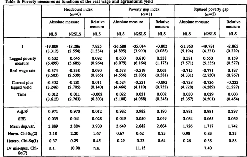
We subjected all these regressions to the same residual diagnostic tests as in section 3.2. All tests were passed comfortably except serial correlation, with indications of significant negative serial correlation in the residuals for all three poverty regressions (for both NLS and N2SLS estimators). On testing for the possibility of omitted lagged effects of some or all of the X, variables from the last survey date, we found that lagged output per acre had a strong effect, similar in size to (and not statistically different from) the effect of current output. On replacing current output per acre by the sum of current and lagged values we obtained the results in Table 3. There was no sign of serial correlation in this model's residuals, for either NLS or N2SLS estimators. All other diagnostic tests passed comfortably. We also deleted the first n

observations or the last n, with n= 1,2,3,4, 5. The results were quite robust to these changes. Our results indicate strong evidence of serial dependence in all three poverty measures, with autoregression coefficients around 0.5-0.6. The real wage rate has a strong short run impact, with a higher elasdcity for the poverty gap index than the headcount index, and highest for the squared poverty gap, indicating strong effects well below the poverty line. The same comment applies to the agricultural yield variable. Direct effects of yield growth on poverty are evident; these may involve either wage-labor employment effects or own-farm productivity gains (as noted, the data do not allow us to distinguish the latter two effects empirically). Controlling

" The lagged poverty measure was multiplied by the NLS estimate of its coefficient raised to the power of the gap between surveys; this provided a good instrument for the first term on the RHS of equation (6).

Table 3: Poverty measures as functions of the real wage and agricultural yield

Headcount index Poverty gap index Squared poverty gap

(xf=O) (a= 1) (a=2)

Absolute measure Relative Absolute measure Relative Absolute measure Relative

measure measure measure

NLS N2SLS NLS NLS N2SLS NLS NLS N2SLS NLS

1 -19.809 -18.286 7.925 -36.688 -35.014 -0.802 -51.360 49.781 -2.865

(3.312) (2.554) (1.334) (4.895) (3.900) (0.088) (5.194) (4.321) (0.229)

Lagged poverty 0.602 0.645 0.092 0.600 0.610 0.338 0.581 0.550 0.159

measure (6.499) (5.685) (0.264) (8.079) (6.164) (1.175) (7.571) (5.335) (0.577)

Real wage rate -0.374 -0.338 0.090 -0.578 -0.519 0.063 -0.715 -0.771 0.187

(3.503) (2.539) (0.865) (4.556) (2.805) (0.381) (4.331) (2.750) (0.767) Current plus -0.302 -0.281 0.011 -0.524 -0.531 -0.092 -0.738 -0.726 -0.233 lagged yield (3.246) (2.705) (0.140) (4.464) (4.110) (0.732) (4.728) (4.289) (1.227) Time 0.012 0.011 -0.002 0.022 0.021 0.002 0.030 0.029 0.003 (3.612) (2.763) (0.803) (5.108) (4.088) (0.345) (5.357) (4.501) (0.454) Adj.R2 0.971 0.970 0.012 0.982 0.982 0.190 0.981 0.981 0.297 SEE 0.039 0.041 0.028 0.049 0.050 0.049 0.064 0.065 0.069 Mean dep.var. 3.889 3.884 3.900 2.649 2.642 2.664 1.726 1.717 1.742 Norm. Chi-Sq(2) 2.18 2.20 1.67 0.67 0.62 0.23 0.98 0.83 0.33 Hetero. Chi-Sq(1) 0.37 0.29 0.45 0.29 0.23 0.64 0.26 0.38 0.88

IV mis-spec. Chi- n.a. 10.98 n.a. 11.15 7.40

Sq(7) Note: See Table 2.

for these variables, there is a significant underlying positive trend, entailing annual rates of increase of 1.2%, 2.2% and 3.0% for headcount index, poverty gap and squared poverty gap.

We also tried the alternative approach analogously to (8). Using the same starting point for the right hand side variables, but adding the one-year lags, and imposing the common factor restrictions we again obtained significant effects of the real wage rate and output per acre, with strong serial dependence in the poverty measures. There were differences, however. The

coefficient on the lagged poverty measures was higher (0.82-0.84 for all three measures), and not significandy less han unity (standard errors of 0.10-0.11), implying explosive long run

properties. Also, the time trend was insignificant. The coefficients on wages and output per acre were also somewhat higher; around 0.62-1.06 for the wage rate and 0.52-1.11 for output per acre, all with t-ratios around four. We rejected these results as implausible.

3.4 Regressions for the real wage rate

Turning to the wage equation, we began with the same variables for X, as used in the poverty regressions. This time the inflation rate was highly significant, though none of the other variables were individually. There was, however, a noticeable loss of fit when all were dropped. Yet log yield was significant when the others were dropped, and none of the others were

significant (except inflation) if they were put back in the equation individually. 7 _{The parameter}

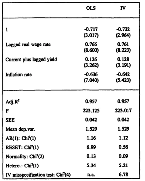
restriction that the coefficients on current and lagged log YNS were equal again passed easily. Table 4 gives both OLS and IV estimates of the final wage equation; the instrumental variables

Table 4: Regressions for real agricultural wage rate

OLS IV

1 -0.717 -0.732

(3.017) (2.964)

Lagged real wage rate 0.766 0.761

(8.600) (8.223)

Current plus lagged yield 0.126 0.128

(3.262) (3.191) Inflation rate -0.636 -0.642 (7.040) (5.423) Adj.R2 0.957 0.957 F 223.125 223.017 SEE 0.042 0.042 Mean dep.var. 1.529 1.529 AR(1): Chi2(1) 1.16 1.12 RESET: Chi2(1) 6.99 0.56 Normality: ChFi(2) 0.13 0.09 Hetero.: Chi2(1) 5.34 5.21

IV misspecification test: ChO2

(4)

Note: 32 annual observations, 1958-89. All variables in logs. Absolute t-ratios in parentheses.

were the two year lagged values of real wages, the price index, output and the time trend. The equations passed the same set of residual diagnostic tests described above.

The dynamic effect is clearly strong, and there is also a sizable short-run adverse effect of inflation. The short-run elasticity of the real wage to output per acre is about 0.13, rising to over eight times that figure in the long-ran. Thus, while we do find strong support for real wage sluggishness, there is a detectable though small short-run impact of current yield.

One can also write this model in terms of the first differences of these variables, augmented with an error correcdon mechanism. The variables of interest-the logs of W, CPI, and YNS-were all stationary in first differences (using both Dickey-Fuller and Augmented Dickey-Fuller tests). Regressing the log wage on the other two variables in levels, the residuals were found to be stationary, implying cointegration and hence the existence of an error-correction model (Engel and Granger (1987):

AInW,

aZAX,

z

X_l)

(10)

On estimating the model in this form one obis (absoblte t-ratios in parentheses):

AnW

-0.637AInCPI

-3.057)

(6.91) (1.37) (255) (5.50) (3.74)

(where R2_{=0.749; SEE=0.043).' However, the parameter restriction needed to yield the same}

model as in Table 4 (namely that 2zt + 2r.3 =0 in obvious notation) performs vray well."'

I The long-rnm price level effect in the error correction term was highly insignificant-indicating that only the real variables matter in the long-run-and was dropped.

3.5

The elasticities

of poverty

to agricultural

yield

The short-run elasticitv of the poverty measure to a change in output per acre is given by

ahnP., - +P M(12)

;s]S= Pa2Y2 + 3(2

8InYNS,

1,

(where the superscripts "YNS" refer to the parameter on log YNS in each equation). The steady-state reduced form of equation (9), as estimated in Tables 3 and 4, gives the poverty measures and real wage rate as a function of agricultural yield per acre and time. Using n_ to denote

steady-state values, the long-run elasticity of the poverty measure to yield is'

alnP,

P2

alnYNVS (1- P,j)0 -Y1) (1 - ,ut)

In each case, the first term on the right-hand-side is the effect operating through the wage rate, while the second reflects other channels, as discussed in Section 2.2.

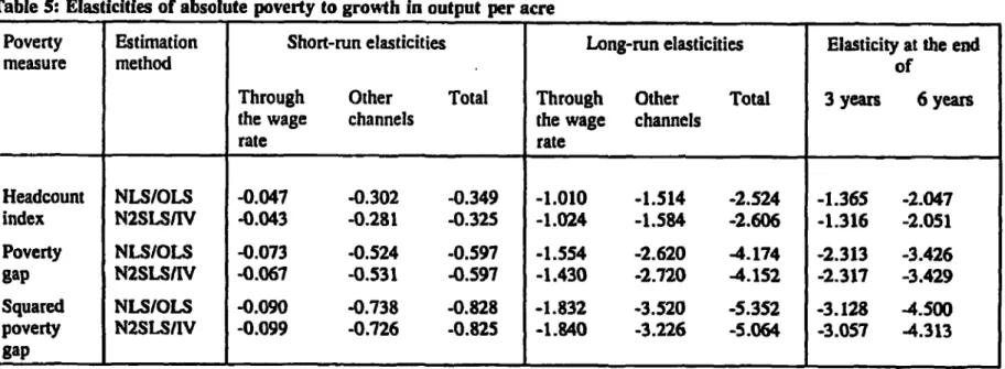
Table 5 gives the elasticities implied by both our estimates from Tables 3 and 4. In the short-run, the growth effect via the wage is small, and dominated by other channels. But in the long-run the wage effects account for about 3040% of the total elasticity. Total elasticities are at least six times higher in the long-run. Half or more of the long-run impact is reached within three years; 80 % is reached in six years. The elasticities are also higher for higher values of a.

The long-mn poverty measures are also an increasing function of time. This presumably reflects an omitted variable, such as population growth, which is difficult to distinguish from time. (Appendix 2 discusses this point further in the context of related work in the literature.)

20 Notice that it is the sum of the current and lagged log YNS on the right hand side of both

the poverty and wage regressions. Thus one collects two terms in log YNS in the steady-state. 17

Table 5: Elasticities of absolute poverty to growth in output per acre

Poverty Estimation Short-run elasticities Long-run elasticities Elasticity at the end

measure method of

Through Other Total Through Other Total 3 years 6 years

the wage channels the wage channels

rate rate Headcount NLS/OLS -0.047 -0.302 -0.349 -1.010 -1.514 -2.524 -1.365 -2.047 index N2SLSIIV -0.043 -0.281 -0.325 -1.024 -1.584 -2.606 -1.316 -2.051 Poverty NLS/OLS -0.073 -0.524 -0.597 -1.554 -2.620 4.174 -2.313 -3.426 gap N2SLSIIV -0.067 -0.531 -0.597 -1.430 -2.720 4.152 -2.317 -3.429 Squared NLS/OLS -0.090 -0.738 -0.828 -1.832 -3.520 -5.352 -3.128 -4.500 poverty N2SLS/IV -0.099 -0.726 -0.825 -1.840 -3.226 -5.064 -3.057 -4.313 gap _

The existence of a positive trend, controlling for yield, implies that without the yield gains over this period, poverty would have increased. Thus the gains to India's rural poor since about

1970-with the incidence of poverty roughly halving between 1970 and 1990 (Appendix 1)-are attributed to yield increases outweighing the underlying adverse trend. From the results in Table 3, one can calculate the minimum rate of growth in output per acre needed assure that poverty does not increase in the long-mn; for the headcount index the minimum rate of yield growth needed is 1.19% per year, while it is 1.30% and 1.27% for the poverty gap and squared poverty gap respectively. The historical rate of growth in yield over this period was 2.32% per year.

3.6

Why are all elasticities

higherfor higher values of ai?

It can be seen in Tables 2, 3 and 5 that the (absolute) elasticities of the poverty measures to both mean consumption and yield are higher for higher values of the parameter a. From (5):

PI = PO('- VIZ); P2 = PII ,[1 '/Z + (a9 (14)

where pP and aP are the mean and standard deviation of consumption by the poor. So the higher elasticity for P, than PO indicates that growth also increases the average consumption of the poor (i.e., that the income gap ratio 1 -

IP/z

21 This least squares estimate using the annual data, with a correction for the (mild) serial

correlation in the OLS error terms.

numbers of) poor. None of this is inconsistent with distribution neutrality overall; for example, all consumption levels could increase at the same rate while the mean consumption of those below the poverty line stays the same or even falls, depending on the density of consumptions in a neighborhood of the poverty line.22

4 Conclusions

India appears to be the only developing country for which consistent poverty measures can be tracked over a long time. We find that measures of absolute rural poverty responded elastically to changes in mean consumption over the period 1958-90. This response vanishes when one focuses on measres of relative poverty; the impact of growth on poverty was roughly distribution-neutral in the long run. Our results strongly reject the "immiserizing growth"

hypotiesis. But nor was there "redistribution with growth".

We have also collated the household survey data with data on agricultural wages and outputs, and estinated a dynamic model determining rural poverty measures and real wages. We find that a range of absolute poverty measures responded in the short run to changes in

agricultural wages as weUl as to average farm yields. And wages responded to farm yields, presumably through effects on labor demand, such as due to multiple cropping. Higher yields

thus helped reduce absolute poverty through induced wage effects, as well as the more direct channels, including effects on both employment and own-farm productivity. The bulk of the consumption gains to poor people since about 1970 are attributed to the direct and indirect impacts of agricultural growth. Nor were the gains confined solely to those near the poverty

2 When all consumptions grow at the same rat, it can be shown that the necessary and

sufficient condition for the absolute elasticity of PI to the mean to be greater ta that of Po is that

line; higher yields also benefited those well below it. However, agricultural growth had no discernable impact on relative poverty. In the short-run, there was also a strongly adverse impact of inflation on real agricultural wages and (hence) absolute poverty.

Neither the consumption-based poverty measures nor real wage rates adjusted

instantaneously. The combined effect of this stickiness in both variables is that the short-ran gains to poor people of labor-demanding productivity growth are far lower than the long-run impacts. Also, the short-run effects operating via the wage rate are minor compared to those operating through other channels. But in the long run, the wage effects do matter, accounting for about 30-40% of the steady-state elasticity of absolute poverty to a yield increase. Overall elasticities in the long run are at least six times higher than the short-run values, and long-run elasticities exceed two for the incidence of poverty, and are over four for the poverty gap indices. Small sample biases entail that (if anything) we have probably underestimated the true long-run elasticities. The process through which India's rural poor participate in the gains from agricultural growth does take time, though about half of the long-run impact occurs within three

years.

Appendix 1: Data sources and estimation methods

Poverty measures

The poverty measures are based on the published National Sample Survey (NSS) data on distributions of per capita monthly expenditure. The distributions are available for 33 NSS rounds, starting with the 3rd round for August 1951-November 1951 and going up to the 47th round for July 1991-December 1991. In keeping with data availability on other variables (see below), the poverty estimates used here are for a shorter period from NSS round 14 (July 1958-June 1959) to round 45 (July 1989-1958-June 1990). The time interval between surveys varies from

11 months to 5.5 years. The poverty line is defined by a per capita monthly expenditure of Rs. 49 in rural areas at October 1973-June 1974 prices. This poverty line was originally proposed by the Task Force on Projections of Minimum Needs and Effective Consumption Demand (Planning Commission 1979), and has recently been endorsed by the Expert Group on Esfimation of

Number and Proportion of Poor (Planning Commission 1993). The deflator we have used to adjust for temporal changes in the cost of living in the rural sector is the Consumer Price Index for Agricultural Laborers (CPI). Point estimates of the poverty measures are constructed using either the beta Lorenz curve of Kakwani (1980) or the general quadratic model of ViDasenor and Arnold (1989), depending on which fits the data best (both satisfied the theoretical conditions needed for a valid Lorenz curve in all survey rounds). Using the formulae in Datt and Ravallion (1992), the poverty measures are calculated from the estimated parameters of the Lorenz curve and the mean per capita consumption expenditure.23 Figure 2 gives the headcount index. A complete series of the poverty measures with a detailed discussion of our methodology and data sources can be found in Datt (1994).

The price index

The CPI for agricultural laborers for the period we cover is compiled from the Labour

Bureau's monthly series on consumer price indices (publisbed in the Indian Labour Journal and the Indian Labour Yearbook.) Beginning September 1964, the index is directly available at the

23 A number of checks are made on the results, including both the theoretical conditions for a valid Lorenz curve, and consistency checks, such as that the estimated value of the bead-count index must lie within the relevant class interval of the published distribution. The estimation echnique has been set-up in a user-friendly computer program which is available on request, so interested readers can readily check our calculations and their sensitvity to our assumptions.

all-India level. For the earlier period, September 1956 through August 1964, however, only state-level indices ar'; available. We have aggregated these into an all-India index using the same weighting diagram as used in the Labour Bureau series for the later period.

A problem with this price index is that the Labour Bureau ignored increases in firewmood prices after 1960-61; firewood is typically a common property resource for agricultural laborers, but it is also a market good, and so the Labour Bureau's practice is questionable.2 4 To test for bias due to this problem we estimated an alternative deflator replacing the firewood sub-series by one based on mean rural firewood prices (only available from 1970) and a series derived by assuming that firewood prices increased at the same rate as all other items in the Fuel and Light category (prior to 1970); Datt (1994) discusses this index furither. Figure 2 also gives the headcount indices and real wages implied by the alternative deflator. We re-estimated the

poverty and wage regressions; the change made little difference to our results (either coefficients or standard errors); elasticities to yield tended to be slightly lower (at most 10% in the long run).

Agricudtural wages

Our data on nominal daily agricultural wages are compiled from Jose (1974, 1988), supplemented with the data reported in the Report of the National Commission on Rural Labour

(Volume 1) [G01, 1991], and Agriculural Wages in India reports since 1984-85. The primary

source of all these data is the Ministry of Agriculture's amnnal publication Agricultural Wages in

India (AWI). The series we use is for male agricultural wages only; data on female agricultural

wages are not available on a consistent basis for the whole period. The AWI data from the aforementioned sources are available as aggregated up to the state level. We have aggregated

these data further to derive an all-India male agricultural wage using state and year specific weights. These weights are constructed as follows.

Ideally, we would have liked to weight the state-level wage rates by the total (or male) state-level agricultural wage employment for that year. However, the data to do this are not available. As a second best, the weights could be constructed as proportional to the nDmber of

total (or male) agricultural laborers in the state. The primary source of data on the latter is from the decenmial censuses. However, even this turns out to be problematic because of the

non-24 The NSS values firewood consumption from own-production at local market prices. Also

see Minhas et al., (1987) for further discussion.

comparability of the definition of "work" in the 1971 census (Krishnamurty, 1984). The more stringent definition in this census actually shows up as a decline in the absolute number of rural workers in many states, when compared with the 1961 census. Our procedure is as follows.

We have comparable state-level data from the NSS on the proportion of agricultural labor households for the years 1956-57, 1964-65, 1974-75, 1977-78, 1983, 1987-88. 2 We use this as a proxy for the proportion of agricultural laborers in the rural population. Next, we combine this with the state-level rural population for these years, estimated by interpolating across the census years, to obtain an estimate of the number of agricultural laborers in different states for these six years. Assuming a constant rate of growth between any two years, we derive amnual estimates of the number of agricultural laborers in each state over the period 1956-57 to 1991-92. The latter expressed as a proportion of the total number of agricultural laborers in all states provides us with the state-year specific weights used in constructing an all-India agricultural wage.

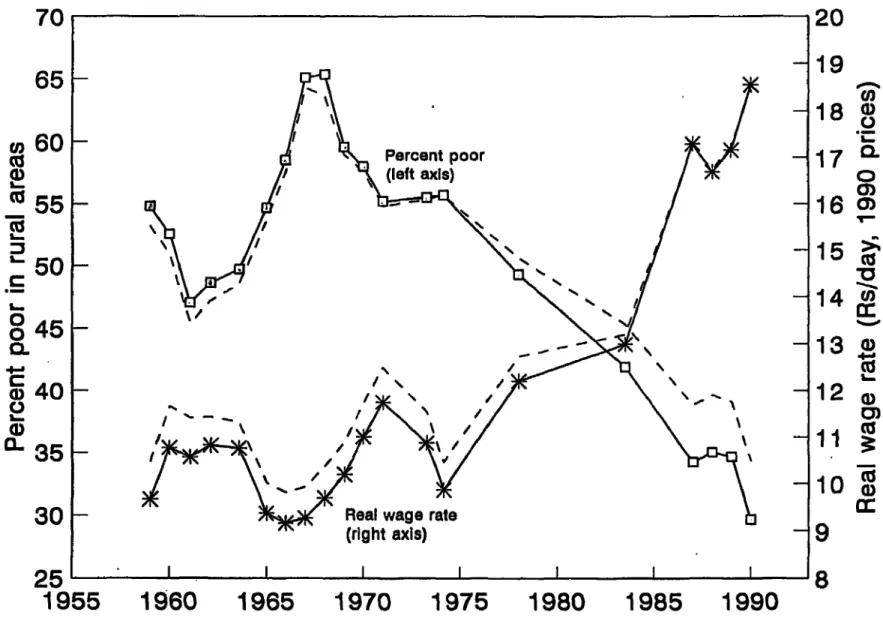
Figure 2 gives the estimated wage rates corresponding to each NSS round.

Agricultural output and area

These data are collated from the Ministry of Agriculture (1993) publication Area and

Production of Principal Crops in India 1991-92. The data are in the form of three annual

indices: (i) the index of agricultural production which is a Laspeyres quantity index of production of all crops, where the weight for a particular crop is given by the average value of that crop's output over the triennium ending 1981-82; (ii) the index of gross cropped area under all crops (including area sown more than once during the year) with the same base period, i.e. the triennium ending 1981-82; and (iii) the index of net sown area also with the same base period. All

three

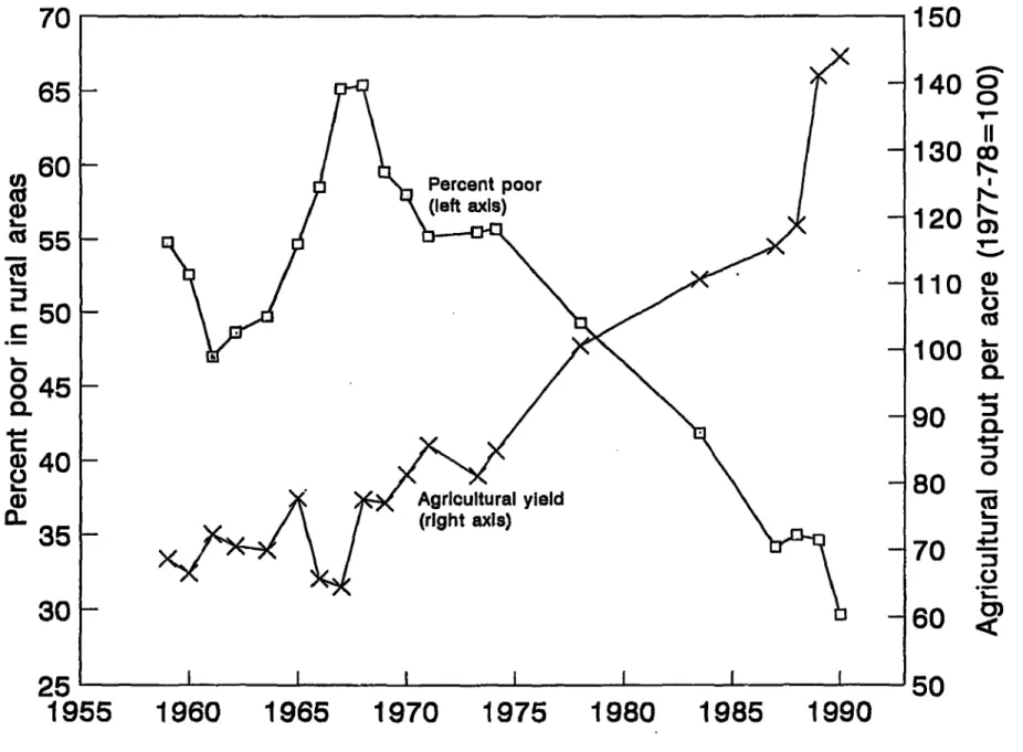
the

Figure 3 gives the index of output per unit net sown area corresponding to each NSS round.

25 These are data from the Second Agricultural Labour Enquiry for 1956-57, the First Rural

Labour Enquiry for 1964-65, the Second Rural Labour Enquiry for 1974-75, and the second, thrd

and fourth Quinquennial Surveys on Employment and Unemployment for 1977-78, 1983 and 1987-88. After 1974-75, Rural Labour Enquiries were integrated with the Qunquennial Surveys. These surveys have adopted a consistent definition of agricultural labor households, viz. rural labor households who derived more than 50% of their income over the preceding year from wage-paid manual labor in agricultural occupations.

Figure 2: Rural Poverty and Agricultural Wages

70

20

65

-1

9

1 83

1x R

60

17

a)F (left axis) 7

30 -

Relwg

aeCu

(ih axs

-98

50-

134a

245

||

13

195

406

196

197

195

180

'285

19

Dashed lines use an alternative deflator (Appendix 1)

0)

25

8~~~~~~~~~~~~~~~~~~~~~.

1955

1960

1965

1970

1975

1980

1985

1990

Figure 3: Rural Poverty and Agricultural Yields

70

150

65

-

140

0

35

U 9

(ri9ht

<

co

60 __6

2

CD

19

19

1100

50

C

8

45

a)40

0

80

35

70~

30

60'

25

50

Population

Annual estinates of the rural population are constructed using census data from all five censuses conducted in the post-independence period. Sectoral populations are assumed to grow at a constant rate between censuses. The population estimates are centered at the beginning of each calendar year which coincides with the mid-point of the corresponding agricultural year.

Marching annual data with NSS rounds

As already noted, the survey periods of the NSS rounds do not always coincide with the agricultural year, nor do aU of them cover a full 12-month period. In adapting the data for the

modelling of poverty by NSS rounds, we have used the following procedure. The data on the CPI are originally colated on a monthly basis and hence permit easy aggregation in the formn of averages over months for the corresponding NSS survey periods. Population estimates were made for the mid-point of each NSS survey period. However, data on the other variables are only available on an anmual basis for each agricultural year. For these variables, we have constructed values corresponding to a given NSS round as (i) the value of the variable for the

agricultral year if the survey period coincides with (or falls entirely within) the agricultural year, or otherwise, as (ii) a weighted average of the values for agricultural years overlapping with the survey period of that round. Thus, for example, for the 18th round, which covers the period February 1963 to January 1964, we construct the corresponding agricultural wage by combining

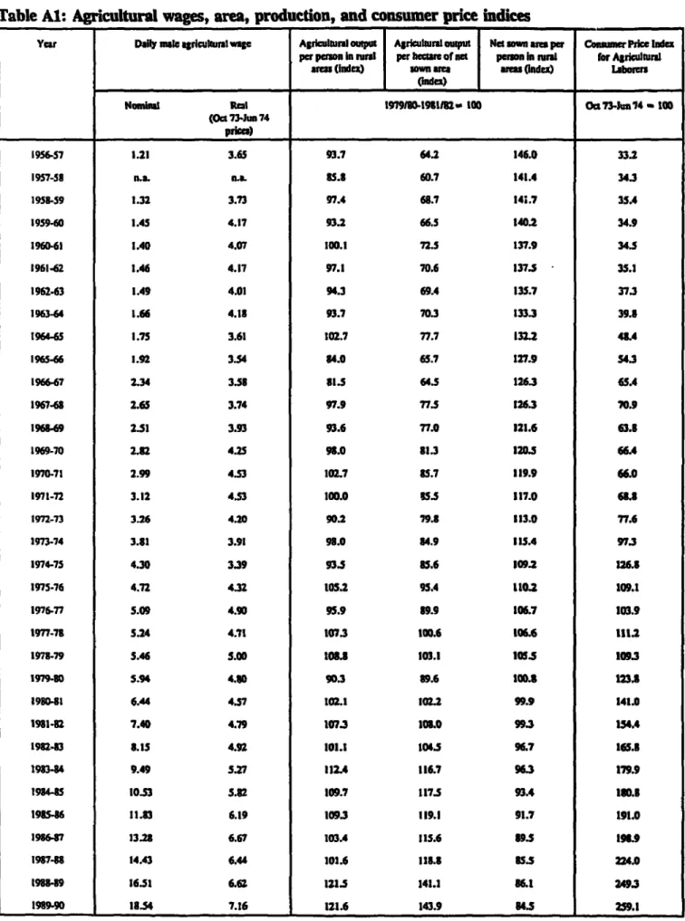
the wage for 1962-63 and 1963-64 in the proportion (5/12) and (7112) respectively. The annual data are in Table Al, while the data by NSS round are given in Table A2.

Appendix 2: Antecedents in the literature

Poverty regressions

Much of the scholarly debate over agricultural growth and rural poverty in India centered on a seminal paper by Ahluwalia (1978), who regressed measures of rural poverty from 12 surveys between 1957 and 1974 against agricultural output per head of tie rural population and a

time trend. He found that higher output was associated with lower poverty, and that there was no trend independendy of this. The debate which followed questioned sensitivity to changes in the period of analysis (Griffin and Ghose, 1979; Saith, 1981). But with only 12 observations,

and relatively little sustained agricultural growth over the period, this may not have been a

Table Al: Agricultural wages, area, production, and consumer price indices

Yeu Daily vale spiculxal wage AgrIuitural eopug Agrulturi Net sown ar per Cormumer Prie lnd pxr womn In mnrsl per heame of nu person h n im for AJrbcult

aas (Index) sown ara am (Index) Labores

N_OInal Real 1979130-19111U2 tO0 Oct73-Ju14 100

(Oct 73-Jun 74 Pim) 1956.57 1.21 3.65 93.7 64.2 146.0 33.2 1957-51 n.a. n. 35.3 60.7 141.4 34.3 1953.59 1.32 3.73 97.4 6i.7 14;.7 35.4 1959.60 1.45 4.17 93.2 66.5 IU.2 34.9 1960-61 1.40 4.07 100.1 72.5 137.9 34.5 1961.62 1.46 4.17 97.1 70.6 137.5 - 35.1 1962.63 1.49 4.01 94.3 69.4 135.7 37.3 1963.64 1.66 4.11 93.7 70.3 1333 39.3 196445 1.75 3.61 12.7 77.7 132.2 41.4 1965-66 1.92 3.54 34.0 65.7 127.9 54.3 1966.67 2.34 3.53 31.5 64.5 1263 6S.4 196741 2.65 3.74 97.9 77.5 126.3 70.9 1961.69 2.51 3.93 93.6 77.0 121.6 63.3 1969-70 2.82 4.25 93.0 31.3 120.5 664 1970-71 2.99 4.53 102.7 3S.7 119.9 6h0 1971-72 3.12 453 100.0 353 117.0 68.3 1972-73 326 4.20 90.2 79.3 113.0 77.6 1973.74 3.81 3.91 98.0 84.9 115.4 973 1974-75 4.30 3.39 93.5 85.6 109.2 26.3 1975-76 4.72 432 105.2 95.4 110.2 109.1 1976.77 5.09 4.90 95.9 39.9 106.7 103.9 1977-73 5.24 4.71 1073 W0.6 106.6 111.2 1973-79 5.46 5.00 103. 103.1 105. 1093 1979-3D 5.94 4.80 90.3 39.6 100.3 123. 19B0.81 6.44 437 101 102.2 99.9 141.0 1931-82 7.0 4.79 107.3 10L0 9.3 154.4 19824.3 3.15 4.92 101.1 104.5 96.7 165.3 198344 9.49 5.27 112.4 116.7 963 179.9 195 10.53 5.82 109.7 117.5 93.4 11.3 195-116 11.83 6.19 1093 119.1 91.7 191.0 193647 13.2 6.67 103.4 ISA.6 39.5 191.9 1987-l 14.43 6.44 102.6 113. U.S 224. 19M1M9 16.51 6.62 IZI.5 141.1 86.1 249.3 1919990 18.54 7.16 121.6 143.9 84.5 259.1

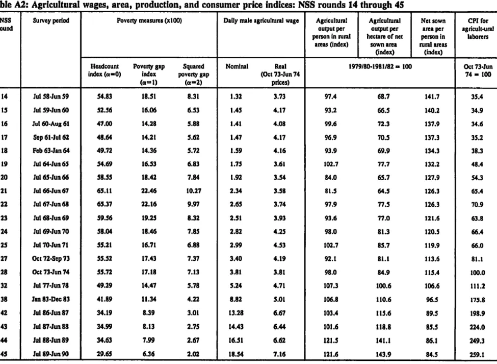
Table A2: Agricultural wages, area, production, and consumer price indices: NSS rounds 14 through 45

NSS Survey period Poverty measures (xlO0) Daily male agricultural wage Agdculturam Agrcultural Net sown CPI for round output per output per area per agncult-ura

person in mral hectare of nct person in laborers

areas (index) sown area rural *reas _______________ (index) (index)

Headcount Poverty gap Squared Nominal Real 1979/80-1981182 100 Oct 73-un index (a-0) Index poverty gap (Oct 73-Jun 74 74 - 100

_(a= 1) (a-2) pnces)

14 Jul S8-Jun 59 54.83 18.51 8.31 1.32 3.73 97.4 68.7 141.7 35.4 IS Jul 59-Jun 60 52.56 16.06 6.53 1.45 4.17 93.2 66.5 140.2 34.9 16 Jul 60-Aus 61 47.00 14.28 5.88 1.41 4.08 99.6 72.3 137.9 34.6 17 Sep 61-Jul 62 48.64 14.21 5.62 1.47 4.17 96.9 70.5 137.3 35.2 18 Feb 63-Jan 64 49.72 14.36 5.72 1.59 4.16 93.9 69.9 134.3 38.3 19 Jul 64-Jun 65 54.69 16.53 6.83 1.75 3.61 102.7 77.7 132.2 48.4 20 Jul 65-1un 66 58.55 18.42 7.84 1.92 3.54 84.0 6S.7 127.9 54.3 21 lul 66-Jun 67 65.11 22.46 10.27 2.34 3.58 81.5 64.5 126.3 65.4 22 Jul 67-Jun 68 65.37 22.16 9.97 2.65 3.74 97.9 77.5 126.3 70.9 23 Jul 68-Jun 69 59.56 19.25 8.32 2.51 3.93 93.6 77.0 121.6 63.8 24 Jul 69-Jun 70 58.04 18.46 7.85 2.82 4.25 98.0 81.3 120.5 66.4 25 Jul 70Jun71 5S.21 16.71 6.88 2.99 4.53 102.7 85.7 119.9 66.0 27 Oct 72-Sep73 55.52 17.43 7.37 3.40 4.19 92.1 81.1 113.6 81.1 28 Oct 73-Jun74 55.72 17.18 7.13 3.81 3.81 98.0 84.9 115.4 100.0 32 Jul 77-Jun 78 49.29 14.47 5.78 5.24 4.71 107.3 100.6 106.6 111.2 38 Jan83-Dec83 41.89 11.34 4.22 8.82 5.01 106.8 110.6 96.5 175.8 42 Jul 86-Jun 87 34.19 8.39 3.01 13.28 6.67 103.4 115.6 89.5 198.9 43 Jul 87-Jun 88 34.99 8.13 2.75 14.43 6.44 101.6 118.8 85.5 224.0 44 Jul 88-Jun89 34.63 7.99 2.67 16.51 6.62 121.5 141.1 86.1 249.3 45 Jul 89-Jun90 29.6S 6.36 2.02 18.54 7.16 121.6 143.9 84.5 259.1

particularly good data set for this purpose (Srinivasan, 1985). The substantial growth that has occurred since then offers hope for a more powerful test (Table 1). Ahluwalia (1985) and Bell and Rich (1994) returned to the Ahluwalia regressions adding data for another year (1977/78) and broadly confirmed his conclusions.26 By adding new data for the 1980s, we have spanned a period of considerably larger changes in all variables though, as noted in section 3.3, our results turn out to be quite robust to changes in the period of analysis-our model estimated on the Ahluwalia (1978) data set would have given similar results. But we have also adopted a rather different model to this literature. This Appendix elaborates on the reasons.

Past work has not tested the distributional effects. Our approach using simulated measures of relative poverty to isolate distributional shifts in the econometric model of poverty measures is new, though it has an antecedent in the method used by Datt and Ravallion (1992) to decompose changes in poverty into growth and redistribution components.27

Higher-order poverLy measures-reflecting distribution below the poverty line-have often been used in the literature, though their role has been rather incidental. Ahluwalia (1978, 1985) and others following him did include the Sen (1976) poverty index, but did not draw out any implications concerning the depth of impacts on the poor. Our results indicate differencs in the impact of productivity growth between these measures, arising from changes in distribution below the poverty line. We find no support for claims that productivity gains in Indian agriculture have by-passed the poorest.

Turning tO the right-hand side variables, almost all past studies of the evolution of India's poverty measures have followed Ahluwalia in using output or income per head. The log of output per person is simply the sum of the logs of output per acre and acres per person, so our specification (initially using both variables) is more general. Our results suggest that thet output effects identified in the literature are to do with yield not land per person. Our finding that lagged output matters, and it has a similar effect as current output, echoes results in Ahluwalia (1985). It is also clear that the output variable is picldng up more than year-to-year fluctuations as Saith (1981) suggests (for then current and lagged output would have opposite signs).

26 Bell and Rich used an earlier version of our data set, rather than Ahluwalia's, and they made

some changes to Ahluwalia's specification, as discussed below.

27 There are other methods of doing such decompositions which do not lend themselves to this

Our long-run elasticity of the headcount index to output per acre is higher than

Ahluwalia's esdmate of the elasticity to agricultural income per person, though the difference is not large; our elasticity is -2.6 (including the wage response; see Table 5), while Ahluwalia (1985) obtained _1.9.2B However, our short-ran elasticity is far lower; while we estimate a

short-run elasticity of -0.3, Ahluwalia (1985) obtained -1.0; the difference appears to reflect the fact that (in common with almost all this literature) Ahluwalia did not include the lagged poverty measure. (We comment fruther on dynamic specification later.) According to our estimates, the impact of growth on the poor is a slower process than Ahluwalia's results suggested, although in the end the impact is even larger than he had predicted.

We have also added real wages. It is odd that the real agricultural wage rate has not figured more prominently in this literature, given how much India's rural poor depend on agricultural labor markets. We know of only one other sudy which nas looked at the impact of the real wage rate on the evolution of rural povertr in India (van de Walle, 1985, using the earlier Ahluwalia poverty measures for 1959-71), though numerous observers have conjectred that this is an important variable (including Acharya and Papanek, 1992). Since this is a very strong predictor in our results, it appears that this may have been an important omitted variable in other studies. If we drop the real wage rate from our model then the NLS estimates of the short-run yield elasticities of poverty to yield rise to -0.41 (t=3.2) for the headcount index

(instead of -0.30), and -1.0 for the squared poverty gap (instead of -0.74).

Saith (1981), Narain (see Desai, 1985) and others (Mathur, 1985; Gaiha, 1989) added the nominal price level to the original Ahluwalia (1978) model.' It is difficult to believe that a monetary variable such as tis could have long-run real effects in a correctly specified model (Bliss, 1985). The price-level effect may well be picking up other omitted income sources or financial assets which matter to the poor (agriultural labor and services, or cash holdings) and are not fully indexed for price changes (Desai, 1985; Bliss, 1985; Sen, 1985). We would conjecture that the significant price level effect identified in the literature largely refect an

1' See equation 5 in Table 7.2 of Ahluwalia (1985). (Since Abluwalia's model is static, the

long-run elasticity for Ahluwalia's model is simply the sum of the coefficients on current and lagged output.) Ahluwalia's augmented model including the price level gives an elasticity of -1.8.

29 In some cases this was the log CPI (Narain), while in others it was the deviation from trend (Saith, Gaiha). But with the trend already included in the regression this difference will only affect the intepretadon of the time trend; we return to this issue.

omitted variable

bias, the key omitted variable being the real wage rate. While we have allowed

short-mn effects of price levels, this proved to be insignificant

once the real wage was added.30

What would a regression

more consistent

with past work look like when estimated on our

extended

series? The Ahluwalia

specification

for the headcount

index gives:

lnP

26.00 - 0.75lnYPCg

- 1.12nYPC,,s -

0.Olt

(4.12) (2.03)

(2.92)

(1.74)

where YPC is agricultural

output per capita. (The RI is 0.81, though there is clearly strong

serial correlation

in the error term, so that this R

and the t-ratios are probably a poor guide to fit

and significance.3 1) The

Narain-Saith

InOP - 122.86 - 0.741lYPC, +0.71lnCPI -0.06t

(2.82) (1.89)

(2.16)

(2.61)

(The R

is 0.77, though there appears to be even stronger serial correlation

in the residuals.

)

An encompassing

model can be used to joindy test our changes

to boti specifications. By adding

both (current and lagged) net sown area per person and the price level (all in logs) to our

preferred model in Table 2, we can do a nested test against the Ahluwalia-Narain-Saith

models.

On doing so we found that all three variables are (highly) insignificant, while the other

coefficients in our poverty model were quite robust, and remained significant at the 5% level or

better.

Our model is more consistent

with the data.

Notice that, in keeping with the literaure, we have mcluded

a time trend, and (as usual)

this is not readily inpretable. The coefficient

on tm depends, of course, on what other

30

Bell and Rich (1994) find significant

effects on the headcount

index of their measure of the

unanticipated

component

of inflation,

though they do not include the real wage rate.

31

The Durbin-Watson

statistic

is 0.80, and the LM tests gives

Chi-square

of 8.08 (significant

at the 0.005 level). Though these tests are not stricty valid given the uneven

spacing, thel- ejectmi

of serial independence

is so strong ta one must be concerned

about inferences

made on the basis

of the OLS standard

errors. The problem of serial correlation

in the errors have been ignoed

this

literatre, even when using data with fairly even spacing.

32

The Durbin-Watson

statistiC

is 0.56, and the LM tests gives a Chi-square

of 9.69.

3

Wald tests convincingly

accept the restriction that the coefficiens on all three variables are

zero; the rejection is even stronger if one adds the restriction that te coefficiet on the lagged

povert measure is also zero.

variables are included; the Ahluwalia-Narain-Saith models above all indicate a negative

coefficient; in our specification the sign switches. Van de Walle (1985) attributed her positive trend to adverse effects of population growth, presumably operating through effects on the distribution of land. This is a conjecture, though a seemingly plausible one.

Aside from the specification of the right-hand side variables, studies in the literature have differed in the assumptions (often implicit) they have made about the dynamic structure of their

models, and the properties of the error term. Virtually all of the regressions in this literature are static. Whilk the shortage of surveys for estimating the poverty measures will entail some small-sample bias in dynamic models, it is plain from our investigation that the true coefficient on

lagged poverty is well above the value of zero that has been widely assumed.

The only other study to allow for serial dependence is Bell and Rich (1994). To deal with the uneven spacing they filled the gaps by two altnative methods: linear interpolation and a forecasting model relating current poverty to its lagged value and current rainfall. They did not use observations after 1977/78, being concerned about the gap to the next round (namely 1983). Aside from o'her differences in specification already noted, our method for dealing with the dynamics has the advantage that we do not lose observations (five would be lost, spanning the

1980s, in which poverty fell considerably). Nor do we need to introduce a separate (and, under the maintained hypotheses, biased) interpolation model in order to estimate the main model.

Wage regressions

Our results are plainly inconsistent with the classic labor surplus theories-there is a detectable effect on real wages of productivity chang