Syracuse University Syracuse University
SURFACE
SURFACE
Dissertations - ALL SURFACE
December 2018
Efficient machine learning: models and accelerations
Efficient machine learning: models and accelerations
Zhe Li
Syracuse University
Follow this and additional works at: https://surface.syr.edu/etd
Part of the Engineering Commons Recommended Citation
Recommended Citation
Li, Zhe, "Efficient machine learning: models and accelerations" (2018). Dissertations - ALL. 989.
https://surface.syr.edu/etd/989
This Dissertation is brought to you for free and open access by the SURFACE at SURFACE. It has been accepted for inclusion in Dissertations - ALL by an authorized administrator of SURFACE. For more information, please contact
ABSTRACT
One of the key enablers of the recent unprecedented success of machine learning is the adoption of very large models with millions of parameters (i.e., weights). The larger-scale model tend to enable the extraction of more complex high-level features, and therefore, lead to a significant improvement of the overall accu-racy. On the other side, the layered deep structure and large model sizes also demand to increase computational capability and memory requirements. In or-der to achieve higher scalability, performance, and energy efficiency for deep learning systems, two orthogonal research and development trends have at-tracted enormous interests. The first trend is the acceleration while the second is the model compression. The underlying goal of these two trends is the high quality of the models to provides accurate predictions. In this thesis, we address these two problems and utilize different computing paradigms to solve real-life deep learning problems.
To explore in these two domains, this thesis first presents the cogent confab-ulation network for sentence completion problem. We use Chinese language as a case study to describe our exploration of the cogent confabulation based text recognition models. The exploration and optimization of the cogent confabu-lation based models have been conducted through various comparisons. The optimized network offered a better accuracy performance for the sentence com-pletion. To accelerate the sentence completion problem in a multi-processing system, we propose a parallel framework for the confabulation recall algorithm. The parallel implementation reduces runtime, improves the recall accuracy by breaking the fixed evaluation order and introducing more generalization, and
maintains a balanced progress in status update among all neurons. A lexicon scheduling algorithm is presented to further improve the model performance.
As deep neural networks have been proven effective to solve many real-life applications, and they are deployed on low-power devices, we then in-vestigated the acceleration for the neural network inference using a hardware friendly computing paradigm, stochastic computing. It is an approximate com-puting paradigm which requires small hardware footprint and achieves high energy efficiency. Applying this stochastic computing to deep convolutional neural networks, we design the functional hardware blocks and optimize them jointly to minimize the accuracy loss due to the approximation. The synthesis results show that the proposed design achieves the remarkable low hardware cost and power/energy consumption.
Modern neural networks usually imply a huge amount of parameters which can not be fit into embedded devices. Compression of the deep learning models together with acceleration attracts our attention. We introduce the structured matrices based neural network to address this problem. Circulant matrix is one of the structured matrices, where a matrix can be represented using a single vector, so that the matrix is compressed. We further investigate a more flexible structure based on circulant matrix, called block-circulant matrix. It partitions a matrix into several smaller blocks and makes each submatrix to be circulant. The compression ratio is controllable. With the help of Fourier Transform based equivalent computation, the inference of the deep neural network can be accel-erated with high energy efficiency on the FPGAs. We also offer the optimization for the training algorithm for block circulant matrices based neural networks to obtain a high accuracy after compression.
EFFICIENT MACHINE LEARNING:
MODELS AND ACCELERATIONS
by Zhe Li
B.S., Beijing University of Posts and Telecommunications, 2012 M.S., Syracuse University, 2014
Dissertation
Submitted in Partial Fulfillment of the Requirements for the Degree of Doctor of Philosophy in Electrical and Computer Engineering
Syracuse University December 2018
Copyright cZhe Li 2018 All Rights Reserved
ACKNOWLEDGEMENTS
During my graduate career, I received help from many people, without whom this dissertation could not have been finished.
First of all, I would like to express my most sincere gratitude to my advi-sor, Dr. Qinru Qiu, who recognized me and offered me the chance of doctorate study on December, 2012 when I hesitated whether to move a step forward in the academia and needed a guidance. She provided comprehensive support all the way through the completion of this degree. Secondly, I am also thank-ful to Dr. Roger Chen, who recognized me and recommended me to seek the doctorate degree when I was a master student in his class. He offered me such opportunity to re-consider my career path. My sincere gratitude also goes to my close collaborator, Dr. Yanzhi Wang, without whom I could not have achieved so much. I learned a lot from his advice and enjoyed the journey we went on together. I would like also to show my appreciation to my committee members, Dr. Sucheta Soundarajan, Dr. Mustafa C. , Dr. Lixin Shen for their valuable feedbacks. I would like to extend my deepest thanks to all my collaborators, Dr. Bo Yuan, Dr. Ji Li, Dr. Jian Tang, Dr. Xue Lin, Siyu Liao, Caiwen Ding, Ao Ren, Ruizhe Cai, Shuo Wang. I would like to thank all my labmates: Dr. Qi-uwen Chen, Dr. Khadeer Ahmed, Wei Liu, Jianwei Cui, Amar Shrestha, Yilan Li, Haowen Fang and Ziyi Zhao. Your support, company and friendship are the treasures during my years in Syracuse.
Finally, I would like to express my everlasting appreciation to my family, who accompanied, encouraged, and supported me in this difficult journey. Without their trusts and constant love, I would never be able to achieve this much. This thesis is dedicated to my wife Lei Zhang, my baby girl Vivian Li, and my parents, Shengzhang Li and Honglei Zou.
TABLE OF CONTENTS Acknowledgements v Table of Contents vi List of Tables ix List of Figures x 1 Introduction 1 1.1 Motivation . . . 1 1.2 Cogent Confabulation . . . 3 1.3 Stochastic Computing . . . 5
1.4 Structured Matrices based Neural Networks . . . 8
1.5 Applications . . . 9
1.5.1 Intelligent Text Recognition System . . . 10
1.5.2 Deep Convolutional Neural Network . . . 11
1.5.3 Recurrent Neural Networks based Automatic Speech Recognition . . . 13
1.6 Contributions . . . 16
2 Cogent Confabulation Assisted Chinese Sentence Completion 19 2.1 Introduction . . . 19
2.2 Formulation of Chinese Completion using Cogent Confabulation 21 2.2.1 Processing the training text . . . 21
2.2.2 Chinese Sentence Confabulation . . . 22
2.3 Training and Recall Algorithm with Case Study . . . 25
2.3.1 Knowledge Link Weighting . . . 28
2.4 Evaluations . . . 29
2.4.1 Necessity of incorporating segmentation labels and circu-lar Knowledge Base . . . 30
2.4.2 Analysis of mutual information . . . 31
2.4.3 Quantified Knowledge Link Weighting scheme . . . 34
2.4.4 Confabulation model optimization . . . 36
2.4.5 Qualitative Results . . . 41
2.5 Conclusion . . . 42
3 Parallel Implementation of Associative Inference for Cogent Confab-ulation 43 3.1 Introduction . . . 43
3.2 Sequential Cogent Confabulation algorithm . . . 45
3.3 Parallel Implementation of Associative Inference . . . 48
3.3.2 Lexicon Level Parallelization . . . 50
3.3.3 Lexicon scheduling for intermittent pruning . . . 52
3.4 Experimental Results . . . 54
3.5 Conclusion . . . 61
4 Highly-Scalable Deep Convolutional Neural Network using Stochas-tic Computing 62 4.1 Introduction . . . 62
4.2 Related Works . . . 66
4.3 Overview of DCNN Architecture and Stochastic Computing . . . 67
4.3.1 DCNN Architecture Decomposition . . . 67
4.3.2 Stochastic Computing (SC) . . . 68
4.3.3 Application-level vs. Hardware Accuracy . . . 71
4.4 Design for Function Blocks and Feature Extraction Blocks . . . 72
4.4.1 Inner Product/Convolution Block Design . . . 72
4.4.2 Pooling Block Designs . . . 76
4.4.3 Activation Function Block Designs . . . 79
4.4.4 Feature Extraction Block Designs . . . 84
4.5 Further Optimization for Function Blocks and Feature Extraction Blocks in HEIF . . . 89
4.5.1 Transmission Gate Based Multiplication . . . 89
4.5.2 APC Optimization . . . 90
4.5.3 Weight Storage Optimization . . . 93
4.5.4 Pipeline Based DCNN Optimizations . . . 98
4.6 Overall Evaluation . . . 100
4.6.1 Optimization Results on Feature Extraction Blocks . . . 100
4.6.2 Overall Results on the DCNNs . . . 105
4.7 Conclusion . . . 108
5 Enabling Efficient Recurrent Neural Networks using Structured Com-pression Techniques on FPGAs 111 5.1 Introduction . . . 111
5.2 Related Work . . . 115
5.3 Structured Compression . . . 116
5.3.1 Block-Circulant Matrix . . . 116
5.3.2 Inference and Training Algorithms . . . 118
5.3.3 Alternating Direction Method of Multipliers (ADMM) Based Training . . . 121
5.4 RNN Model Design Exploration: A software view . . . 123
5.5 FPGA Acceleration . . . 127
5.5.1 FFT/IFFT Decoupling . . . 127
5.5.2 Datapath and Activation Quantization . . . 129
5.5.3 Operator Scheduling . . . 131
5.6 Hardware Design . . . 136
5.6.1 E-RNN Hardware Architecture . . . 136
5.6.2 PE Design . . . 137
5.6.3 Compute Unit (CU) Implementation . . . 138
5.7 Experiment Evaluation . . . 143
5.8 Conclusion . . . 148
6 Conclusion and future work 149 6.1 Conclusion . . . 149
6.2 Future Directions . . . 150
6.2.1 Applying Structure Matrices to DCNN . . . 150
6.2.2 Accelerating structured matrices on GPGPU . . . 151
Bibliography 152
LIST OF TABLES
2.1 Penn Treebank tag list. . . 21
2.2 Comparison of non-circular and circular model. . . 31
2.3 Knowledge link grouping. . . 35
2.4 Example of confabulated sentences. . . 41
4.1 Absolute Errors of OR Gate-Based Inner Product Block . . . 74
4.2 Absolute Errors of MUX-Based Inner Product Block . . . 74
4.3 Relative Errors of the APC-Based Compared with the Conven-tional Parallel Counter-Based Inner Product Blocks . . . 76
4.4 Relative Result Deviation of Hardware-Oriented Max Pooling Block Compared with Software-Based Max Pooling . . . 79
4.5 The Relationship Between State Number and Relative Inaccu-racy of Stanh . . . 80
4.6 The designs of FEBs and corresponding optimization functions . 88 4.7 Comparison of inner-product blocks before and after optimiza-tion using1024-bit-stream. . . 93
4.8 Hardware performance of FEBs with the different input sizes us-ing1024-bit-stream w/ and w/o pipeline based optimization . . 99
4.9 Comparison among various hardware-based and software-based DCNNs . . . 102
4.10 Comparison among Various SC-DCNN Designs Implementing LeNet 5 . . . 106
4.11 Application-level performance and hardware cost of LeNet-5 implementation using the proposed HEIF. . . 106
4.12 Comparison with existing hardware platforms for handwritten digit recognition using the MNIST [27] dataset . . . 107
4.13 List of existing hardware platforms for image classification using (part of) the AlexNet [63] on ImageNet [26] dataset . . . 108
5.1 Comparison among LSTM based RNN models. . . 125
5.2 Comparison among GRU based RNN models. . . 125
5.3 Comparison of two selected FPGA platforms . . . 143
5.4 Detailed comparisons for different (LSTM and GRU) RNN de-signs on FPGAs (ours, ESE, and C-LSTM). . . 144
LIST OF FIGURES
1.1 Stochastic multiplication using: (a) unipolar encoding (b) bipolar
encoding. . . 6
1.2 Scaled addition in stochastic computing. . . 7
1.3 Overall architecture of the ITRS models and algorithmic flow. . . 11
1.4 General DCNN architecture. . . 12
1.5 An LSTM based RNN architecture. . . 13
1.6 A GRU based RNN architecture. . . 14
2.1 Lexion Structure of confabulation model. . . 26
2.2 Lexion Structure of confabulation model (Any arrow is from source lexicon to target lexicon. Orange arrows represents Knowledge Links from observable lexicons to unobservable or partially observable lexicons; Green arrows represents Knowl-edge Links between lexicons in same level; Blue arrows repre-sents Knowledge Links from unobservable or partially observ-able lexicons to observobserv-able lexicons). . . 27
2.3 Recall accuracy of sentence confabulation model with/without segmentation label . . . 30
2.4 Mutual information trend chart for 4 kinds of Knowledge Links. 32 2.5 Recall accuracy of different training set size. . . 33
2.6 Knowledge Links’ mutual information. . . 34
2.7 Recall Accuracy of basic confabulation model of different bandgap value with/without weighting. . . 36
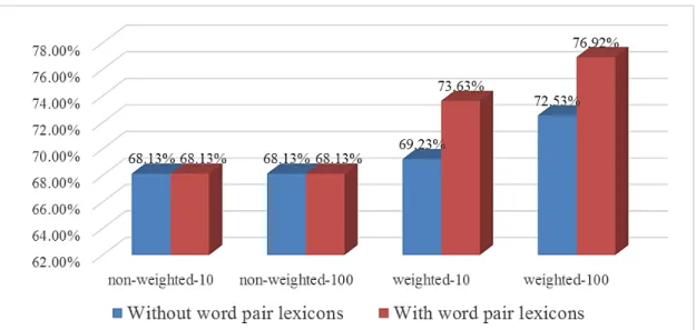
2.8 Recall Accuracy of confabulation model with/without word pair lexicons (non-weighted-10 represents recall accuracy with bandgap value of 10 and without weighting scheme; non-weighted-100 represents recall accuracy with bandgap value of 100 and without weighting scheme; Weighted-10 represents re-call accuracy with bandgap value of 10 and weighting scheme; Weighted-100 represents recall accuracy with bandgap value of 100 and weighting scheme). . . 37
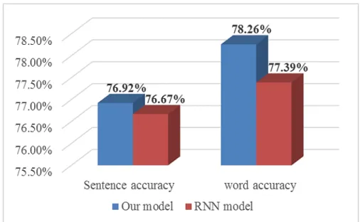
2.9 Recall accuracy between different models(sentence accuracy is evaluated by the amount of sentences recalled identically to orig-inal sentences; word accuracy is evaluated by the amount of missing Chinese charaters recalled identically to the original). . . 38
2.10 Recall accuracy of tags and segmentation labels(Overall denotes accuracy for all characters in sentences; Unknown denotes accu-racy for unknown missing characters, Known denotes accuaccu-racy for known characters). . . 39
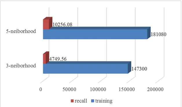
2.11 Training time and recall time of different KL structure. . . 40
3.2 Parallel confabulation architecture on lexicon level . . . 50
3.3 Sentence lexicon model example . . . 55
3.4 Compute time for RLP and LLP w/o intermittent pruning . . . . 56
3.5 Sentency accuracy for RLP and LLP w/o intermittent pruning . 57 3.6 Compute time for LLP w/o and w/ intermittent pruning . . . . 58
3.7 Sentency accuracy for LLP w/o and w/ intermittent pruning . . 58
3.8 Compute time for LLP w/ intermittent pruning for different lex-icon thread pool sizes . . . 59
3.9 Sentence accuracy for LLP w/ intermittent pruning with differ-ent lexicon thread pool sizes . . . 59
3.10 Compute time for LLP w/ intermittent pruning on 8-core CPU machine and 16-core CPU machine with 20 lexicon threads . . . 60
4.1 Three types of basic operations (function blocks) in DCNN. (a) Inner Product, (b) pooling, and (c) activation. . . 68
4.2 Stochastic multiplication. (a) Unipolar multiplication and (b) bipolar multiplication. . . 71
4.3 Stochastic addition. (a) OR gate, (b) MUX, (c) APC, and (d) two-line representation-based adder. . . 71
4.4 Stochastic hyperbolic tangent. . . 72
4.5 16-bit Approximate Parallel Counter. . . 75
4.6 The Proposed Hardware-Oriented Max Pooling. . . 79
4.7 Output comparison of Stanh vs tanh. . . 80
4.8 Diagram of the proposed ReLU block. . . 82
4.9 The structure of a feature extraction block. . . 85
4.10 Structure of optimized Stanh for MUX-Max-Stanh. . . 86
4.11 XNOR gate implementations. (a) Static CMOS design, (b) Trans-mission gate design. . . 90
4.12 (a) Redesigned 16-input APC structure, (b) Redesigned 25-input APC structure. . . 91
4.13 Filter-Aware SRAM Sharing Scheme. . . 95
4.14 Application-level error rates for (a) clustering through all layers, (b) clustering within each layer and layer-wise clustering. . . 97
4.15 Two-tier pipeline design in the framework. . . 98
4.16 Imprecision for Optimized FEBs with bit-stream length L = 256,512,1024 . . . 101
5.1 Block-circulant matrices for weight representation. . . 118
5.2 An illustration of FFT-based calculation in block-circulant matrix multiplication. . . 119
5.3 Euclidean mapping for a 4×4 matrix with block size of 2. . . 123
5.4 The overall procedure of ADMM-based structured matrix training.123
5.5 An illustration of the (a) circulant convolution operator; (b) its
5.6 Piece-wise linear activation functions. . . 131
5.7 Computational complexity of LSTM operators. . . 132
5.8 Illustration of operator scheduling on data dependency graph.
The circle represents the element-wise operator, and the square represents the circulant convolution operator. . . 132
5.9 The overall E-RNN hardware architecture. . . 137
5.10 The PE design in FPGA implementation. . . 138 5.11 One compute unit (CU) with multiple processing elements (PEs)
of LSTM. . . 139 5.12 A compute unit (CU) with multiple processing elements (PEs) of
GRU. . . 140 5.13 Overview of high level synthesis framework. . . 141
CHAPTER 1 INTRODUCTION
From the end of the first decade of the 21st century, neural networks have been experiencing a phenomenal resurgence thanks to the big data and the significant advances in processing speeds. Large-scale deep neural networks (DNNs) have been able to deliver impressive results in many challenging prob-lems. For instance, DNNs have led to breakthroughs in object recognition ac-curacy on the ImageNet dataset [26], even achieving human-level performance for face recognition [117]. Such promising results triggered the revolution of several traditional and emerging real-world applications, such as self-driving systems [51], automatic machine translations [22], drug discovery and toxicol-ogy [13]. As a result, both academia and industry show the rising interests with significant resources devoted to investigation, improvement, and promotion of deep learning methods and systems.
In this chapter, we discuss the motivation of the study. Then we introduce the basics of three computing paradigms for machine learning models espe-cially deep learning models. Applications of different learning systems are in-troduced. Finally, the contributions of the thesis are reviewed.
1.1
Motivation
Machine learning technology benefits many aspects of modern life: web
searches, e-commerce recommendations, social network content filtering, etc.
[67]. Unfortunately, the conventional machine learning techniques were re-stricted due to the lack of ability to automatically extract high-level features.
These features traditionally have been extracted by well-engineered manual
fea-ture extractors.Deep learningmethods have taken advantage of the architecture
of multi-level representations to learn very complex functions [67]. Here, each representation is obtained from a slightly less abstract level through the trans-formation based on a simple non-linear module. Deep learning significantly enhances the machine learning capability using learning from data by these multiple layers for different features without human involvement.
Due to the deep structure, the performance of deep learning model highly relies on the capability of hardware resources. From high performance server
clusters [25, 14] to General-Purpose Graphics Processing Units (GPGPUs) [54, 9],
parallel accelerations of deep neural networks (DNNs) are widely used in both
the academic and industry. Recently, hardware acceleration for DNNs has
at-tracted enormous research interests onField-Programmable Gate Arrays (FPGAs)
[138, 89, 93]. Nevertheless, there is a trend of embedding DNNs into light-weight embedded and portable systems, such as surveillance monitoring sys-tems [52], self-driving syssys-tems [51], unmanned aerial syssys-tems [87], and robotic systems [62]. These scenarios require very low power & energy consumptions and small hardware footprints. Besides, cell phones [67] and wearable devices [41] equipped with hardwalevel neural network computation capability re-quire the radical reduction in power & energy consumptions and footprints.
This thesis mainly addresses the inference acceleration and model compres-sion for modern machine learning models. The acceleration also implies an energy-efficient system that enables the models to run on low-power devices. Meanwhile, effective modeling and training optimization for specific applica-tions are proposed to maintain a good accuracy. We investigate three
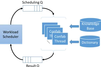
com-puting paradigms to explore the efficient machine learning model acceleration. The first one, Cogent Confabulation is an application oriented acceleration re-search, which is introduced in Chapter 2 and Chapter 3. The second computing paradigm in this thesis is Stochastic Computing, which is more general to neu-ral networks, is described in Chapter 4. The last computing paradigm is the structured matrices based neural network acceleration and model compression, which is presented in Chapter 5.
1.2
Cogent Confabulation
Inspired by human cognitive process, cogent confabulation [47] mimics human information processing including Hebbian learning, correlation of conceptual symbols and recall action of brain. Based on the theory, the cognitive informa-tion process consists of two steps: learning and recall. The confabulainforma-tion model represents the observation using a set of features. These features construct the basic dimensions that describe the world of applications. Different observed at-tributes of a feature are referred as symbols. The set of symbols used to describe the same feature forms a lexicon and the symbols in a lexicon are exclusive to each other. In learning process, matrices storing posterior probabilities between
neurons of two features are captured and referred as theknowledge links (KL).A
KL stores weighted directed edges from symbols in source lexicon to symbols in target lexicon. The(i, j)th entry of a KL, quantified as the conditional probabil-ity P(si|tj), represents the Hebbian plasticity of the synapse betweenith symbol
in source lexicon sand jthsymbol in target lexicont. The knowledge links are
constructed during learning process by extracting and associating features from
knowl-edge base (KB). During recall, the input is a noisy observation of the target. In this observation, certain features are observed with great ambiguity, therefore multiple symbols are assigned to the corresponding lexicons. The goal of the recall process is to resolve the ambiguity and select the set of symbols for max-imum likelihood using the statistical information obtained during the learning process. This is achieved using a procedure similar to the integrate-and-fire mechanism in biological neural system. Each neuron in a target lexicon receives an excitation from neurons of other lexicons through KLs, which is the weighted sum of its incoming excitatory synapses. Among neurons in the same lexicon, those that are least excited will be suppressed and the rest will fire and become excitatory input of other neurons. Their firing strengths are normalized and proportional to their excitation levels. As neurons gradually being suppressed, eventually only the neuron that has the highest excitation remains firing in each
lexicon and the ambiguity is thus resolved. Letldenote a lexicon,Fl denote the
set of lexicons that have knowledge links going into lexiconl, andSl denote the
set of symbols that belong to lexiconl. The excitation of a symbol tin lexiconl
is calculated by summing up all incoming knowledge links:
el(t)=X k∈Fl X s∈Sk [el(s)ln(P(s|t) p0 )]+B,t∈Sl (1.1)
where the functionel(s)is the excitation level of the source symbol s. The param-eter p0is the smallest meaningful value ofP(si|tj). The parameterBis a positive
global constant called the bandgap. The purpose of introducing Bin the
func-tion is to ensure that a symbol receiving N active knowledge links will always
have a higher excitation level than a symbol receiving(N−1)active knowledge
links, regardless of their strength. As we can see, the excitation level of a symbol is actually its log-likelihood given the observed attributes in other lexicons.
1.3
Stochastic Computing
Deviated from the conventional binary computing (referred asconventional
com-puting),stochastic computing (SC) represents any number using a stream of bits.
Here the value of real number x in the unit interval is interpreted by the ratio
of bit-1 in the entire bit-stream, i.e., P(X = 1). For instance, the 8-bit sequence 00100101 containing three 1s denotesx=P(X =1)= 38 =0.375. Since each bit has the same weight, number representation in stochastic computing is unary and hence enables different interpretations for the same value. Besides this unipolar coding format [34], bipolar coding format [34] is another popular number repre-sentation scheme in stochastic computing. In the scenario of bipolar coding, the relationship between xand P(X = 1)becomes P(X = 1)= x+21, which enables the stochastic representation for negative number. Notice that for either unipolar or bipolar coding format, the represented number ranges in[0,1]or[−1,1]. To represent a number beyond this range, a pre-scaling operation [135] or integer bit-stream based representation [6] can be used to relax this constraint.
A major advantage of stochastic computing is its ultra-low hardware cost: Many complicated arithmetic functions can now be implemented with very simple logic circuits. For instance, as shown in Figure 1.1, the real multiplication
can be performed with anANDgate in the unipolar coding form since
c= P(C= 1)
= P(A= 1)P(B= 1)
axb a b a b axb (a) (b)
Figure 1.1: Stochastic multiplication using: (a) unipolar encoding (b) bipolar encoding.
or with anXNORgate in bipolar coding form since
c=2P(C =1)−1
=2[P(A=1)P(B=1)+P(A= 0)P(B= 0)]−1
=2[P(A=1)P(B=1)+(1−P(A= 1))(1−P(B=1))]−1
=(2P(A=1)−1)(2P(B=1)−1)
=ab.
Another example is regarding the adder, which can be simply implemented with a multiplexer (see Figure 1.2) in the scenario of stochastic computing, for
c= P(C =1) = 1 2(P(A=1)+ 1 2P(B=1) = 1 2(a+b).
Additionally, the addition in the bipolar form uses this multiplexer as well, since
c=2P(C =1)−1 =2[1 2(P(A=1)+ 1 2P(B=1)]−1 = 1 2[2P(A=1)−1)+(2P(B= 1)−1)] = 1 2(a+b).
½ bit stream (a+b)/2 a b M U X
Figure 1.2: Scaled addition in stochastic computing.
signal sensing and processing in wearable devices. Besides, the abundant bud-get on area offers immense design space in optimizing hardware performance in terms of power, latency and speed via efficient trade-offs between area and those metrics, thereby implying the potential application of stochastic comput-ing in large-scale systems that requires massive parallelism for basic computcomput-ing units.
Another advantage of stochastic computing is its inherent error-resilience. By nature, the redundant representation of stochastic computing translates to the strong capability for tolerating transient error and soft error (bit-flipping) since each bit has the same weight in bit-stream. For instance, as reported in [97, 85, 134], compared to their conventional computing counterparts, the stochastic digital signal processing component shows much better error-resilience capa-bility, which is attractive for the emerging noise-rich deep nanoscale CMOS era.
1.4
Structured Matrices based Neural Networks
In general, a circulant matrix W ∈ Rn×n [94] is defined by a vector w =
(w1,w2, . . . ,wn)as the following: W= w1 wn . . . w3 w2 w2 w1 wn w3 ... w2 w1 ... ... wn−1 ... ... wn wn wn−1 . . . w2 w1 . (1.2)
From equation (1.2) it is seen that ann-by-ncirculant matrix only hasn
param-eters because of its strong structure. Clearly, when such structure is imposed to the weight matrices of DNNs, the required space cost for storing the weights is immediately reduced fromO(n2)toO(n).
Besides the advantage on low space cost, the use of circulant matrices as weight matrices can also lead to low computational complexity for both infer-ence and training, which are described as below:
Inference:The dominating computation during the forward propagation in
the inference is the matrix-vector multiplication (Wx). According to [94], when
Wis a circulant matrix,Wxcan be performed as below:
a=Wx=IDFT(DFT(w)◦DFT(x)), (1.3)
where ◦ denotes the element-wise multiplication; DFT(·) denotes the Discrete
Fourier transform; and IDFT(·) denotes the inverse Discrete Fourier transform.
Notice that since the computational complexity of n-point DFT/IDFT is only
O(nlogn), the computational complexity of DNN inference can achieve
Training: For backward propagation in the training, recall that its key pro-cedure is to perform the chain rule-based calculation for the gradient of loss
functionLwith respect to the weight vectorwas below:
∂L ∂w = ∂L ∂a ∂a ∂w, (1.4) where ∂L
∂a is the gradient back-propagated from the subsequent layer. Notice
that in the scenario thatWis a square circulant matrix, as indicated in [18], ∂w∂a
is a circulant matrix defined by the vector x0 = (x
1,xn,xn−1, . . . ,x2). Therefore, according to [94], equation (1.4) can be simplified as below:
∂L ∂w =IDFT(DFT( ∂L ∂a)◦DFT(x 0 )), (1.5)
where 1 is a column vector full of ones. In addition, the gradient of input x
which is back-propagated to the previous layer, should be calculated as:
∂L ∂x = ∂L ∂a ∂a ∂x. (1.6)
Notice that here ∂∂xa is also a circulant matrix that is defined as w0 =
(w1,wn,wn−1, . . . ,w2). Hence equation (1.6) can also be simplified as below:
∂L ∂x = IDFT(DFT( ∂L ∂a)◦DFT(w 0 )). (1.7)
From equation (1.5) and (1.7) it is seen that, whenW is a circulant matrix, the
updating scheme for the gradients ofwandx, as the key part of DNN training,
can also be calculated using DFT/IDFT, thereby rendering order-of-magnitude reduction in computational cost for training (fromO(n2)toO(nlogn)).
1.5
Applications
be-telligent Text Recognition System (ITRS); Stochastic Computing is applied on the
deep convolutional neural networks (DCNNs)and structured matrices based
neu-ral network is used to train theRecurrent Neural Networks (RNNs)forautomatic
speech recognition (ASR).
1.5.1
Intelligent Text Recognition System
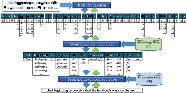
In a recent development, the cogent confabulation model was used for sen-tence completion [47, 101]. Trained using a large amount of literature, the confabulation algorithm has demonstrated the capability of completing a sen-tence (given a few starting words) based on conditional probabilities among the words and phrases. We refer these algorithms as the “association” models. The brain inspired signal processing flow could be applied to many applica-tions. A proof-of-concept prototype of context-aware Intelligence Text Recogni-tion system (ITRS) is developed on high performance computing cluster [100]. As shown in Figure 1.3, the lower layer of the ITRS performs pattern matching of the input image using a simple non-linear auto-associative neural network model called Brain-State-in-a-Box (BSB) [4]. It matches the input image with the stored alphabet. A race model is introduced that gives fuzzy results of pattern matching. Multiple matching patterns will be found for one input character image, which is referred as ambiguity. The upper layer of the ITRS performs information association using the cogent confabulation model [47]. It enhances those BSB outputs that have strong correlations in the context of word and sen-tence and suppresses those BSB outputs that are weakly related. In this way, it selects characters that form the most meaningful words and sentences.
beginning
but to perceive that the handcuffs were not for me b e g i n n i n g p e r c e i v e b u t t o t h a t t h e h a n d c u f f s w e r e n o t f o r me BSB Recognition a e s l g n s e n e m n h g a o e c s t v l i x a s w t e t s h b f h w s u o t n d a i o u
Word Level Confabulation
besieging believing beginning banishing ... porceite perceive parseile twit that text test ... the she handcuffs fere sere were here ... nut nun nod not ... fur fir far for but to me b u t b i i n t o p r e i e t t h e a n d c u f f s e r e n f r m e
Sentence Level Confabulation
...but beginning to perceive that the handcuffs were not for me ...
Knowledge Base (KB) Knowledge Base (KB) ... ... ... ... ... ... ... ... ... ... ... ... ... ... ... ... ...but beginning to perceive that
the handcuffs were not for me ....
Figure 1.3: Overall architecture of the ITRS models and algorithmic flow.
1.5.2
Deep Convolutional Neural Network
Deep Convolutional Neural Networks (DCNN) are biologically inspired
vari-ants of multi-layer perceptrons (MLPs) by mimicking the animal visual
mecha-nism [50]. Thus, a DCNN has special sets of neurons only connected to a small receptive field of its previous layer rather than fully connected. Besides an in-put layer and an outin-put layer, a general DCNN architecture consists of a stack ofconvolutional layers, pooling layers, and fully connected layersshown in Figure 1.4. Please note that some special layers like normalization or regularization are not the focus in this thesis.
1) A convolutional layer is associated with a set of learnable filters (or
ker-nels) [68], which are activated when specific types of features are found at some spatial positions in the inputs. Filter-sized moving windows are applied to the inputs to obtain a set of feature maps by calculating the convolution of the filter
Fully connected layers
}
Pooling Layers Convolutional layers Input layers Output layersFigure 1.4: General DCNN architecture.
pixel in a feature map, takes a set of inputs and corresponding filter weights to calculate their inner-products.
2)After extracting features using convolution, a subsampling step can be
ap-plied to aggregate statistics of these features to reduce the dimensions of data and mitigate over-fitting issues. This subsampling operation is realized by a
pooling neuronin pooling layers, where different non-linear functions can be ap-plied, such as max pooling, average pooling, and L2-norm pooling. Among them, max pooling is the dominating type of pooling in state-of-the-art DC-NNs due to the higher overall accuracy and convergence speed. The activa-tion funcactiva-tions are non-linear transformaactiva-tion funcactiva-tions, such as Rectified Lin-ear Units (ReLU) f(x) = max(0,x), hyperbolic tangent (tanh) f(x) = tanh(x) or
f(x) = |tanh(x)|, and sigmoid function f(x) = 1+1e−x. Among them, the ReLU
function is the dominating type in the (large-scale) DCNNs due toi) the lower
complexity for software implementation; and ii) the reduced vanishing
gradi-ent problem [37]. These non-linear transformations are conducted somewhere before the inputs of the next layer, ensuring that they are within the range of
[−1,1]. Usually, a combination of convolutional neurons, pooling neurons and
g i h f o ct-1 gt it ft Recurrent Projection Input xt ct ot yt-1 mt Output Memory Block Cell
Figure 1.5: An LSTM based RNN architecture. abstraction from the input images or previous low-level features.
3) A fully connected layer is a normal neural network layer with its inputs
fully connected with its previous layer. Eachfully connected neuroncalculates the
inner-product of its inputs and corresponding weights.
1.5.3
Recurrent Neural Networks based Automatic Speech
Recognition
Long short-term memory (LSTM)
Modern large scale Automatic Speech Recognition (ASR) systems take advan-tage of LSTM-based RNNs as their acoustic models. An LSTM model consists of large matrices which is the most computational intensive part among all the steps of the ASR procedure. We focus on a representative LSTM model
presented in [109] whose architecture is shown in Figure 1.5. An
LSTM-based RNN accepts an input vector sequence X = (x1;x2;x3;...;xT) (each of xt
is a vector corresponding to time t) with the output sequence from last step
z
r
c
tc
t-1x
tr
tz
tc
t~
Figure 1.6: A GRU based RNN architecture.
Y = (y1;y2;y3;...;yT)by using the following equations iteratively from t = 1 to
T: it = σ(Wixxt+Wiryt−1+Wicct−1+bi), (1.8a) ft = σ(Wf xxt +Wf ryt−1+Wf cct−1+bf), (1.8b) gt = σ(Wcxxt+Wcryt−1+bc), (1.8c) ct = ftct−1+gtit, (1.8d) ot = σ(Woxxt +Woryt−1+Wocct+bo), (1.8e) mt = oth(ct), (1.8f) yt = Wymmt, (1.8g)
where symbols i, f, o, c, m, and y are respectively the input gate, forget gate,
output gate, cell state, cell output, and projected output [109]; the operation
denotes the point-wise multiplication, and the+ operation denotes the
point-wise addition. The W terms denote weight matrices (e.g. Wix is the matrix
of weights from the input vector xt to the input gate), and theb terms denote
bias vectors. Please noteWic, Wf c, andWoc are diagonal matrices for peephole
connections [36], thus they are essentially a vector. As a result, the matrix-vector multiplication likeWicct−1can be calculated by theoperation. σis the logistic
hyperpolic tangent (tanh) activation function ash.
In the above equations, we have nine matrix-vector multiplications
(exclud-ing peephole connections which can be calculated by ). In one gate/cell,
W∗xxt +W∗ryt−1 can be combined/fused in one matrix-vector multiplication by concatenating the matrix and vector as W∗(xr)[xTt,y
T t−1]
T. Furthermore, the four
gate/cell matrices can also be concatenated and calculated through one matrix-vector multiplication as W(i f co)(xr)[xTt ,y
T t−1]
T
. In this way, we can compute the above equations with only two matrix-vector multiplications, i.e. W(i f co)(xr) [xT t ,y T t−1] T andWymmt.
Gated recurrent units (GRU)
The GRU is a variation of the LSTM as introduced in [20]. It combines the for-get and input gates into a single “update gate”. It also merges the cell state and hidden state, and makes some other changes. The architecture is shown in Figure 1.6. Similarly, it follows equations iteratively fromt=1toT:
zt =σ(Wzxxt+Wzcct−1+bz), (1.9a)
rt =σ(Wrxxt+Wrcct−1+br), (1.9b)
˜ct =h(Wcx˜ xt+Wcc˜ (rtct−1)+bc˜), (1.9c)
ct =(1−zt)ct−1+zt ˜ct (1.9d)
where symbolsz, r, ˜c, care respectively the update gate, reset gate, reset state,
and cell state; theoperation denotes the point-wise multiplication, and the+
operation denotes the point-wise addition. TheWterms denote weight matrices
we use tanh activation function ash. Note that a GRU has two gates (update and reset), while an LSTM has three gates (input, forget, output). GRUs do not have the output gate that is present in LSTMs. Instead, the cell state is taken as
the output. The input and forget gates are coupled by an update gatez, and the
reset gateris applied directly to the previous cell state.
In the above set of equations, we have six matrix-vector multiplications. In the reset and update gates,W∗xxt+W∗cct−1can be combined/fused in one matrix-vector multiplication by concatenating the matrix and matrix-vector asW∗(xc)[xTt ,c
T t−1]
T
. Furthermore, the reset and update gate matrices can also be concatenated and calculated through one matrix-vector multiplication asW(rz)(xc)[xTt ,c
T t−1]
T
. In this way, we compute the above equations with three matrix-vector multiplications, i.e.W(rz)(xc)[xTt,c T t−1] T,W ˜ cxxt, andWcc˜ (rtct−1).
1.6
Contributions
This thesis studies the inference acceleration for modern machine learning mod-els with high accuracy performance. We investigate three computing paradigms to explore the efficient machine learning model acceleration. The organization and contributions of this thesis are concluded as the following.
1. Cogenet confabulation based models on the text recognition system have been investigated and optimized in [77, 98, 99] to offer the state-of-the-art quality. In Chapter 2, we used Chinese language sentence completion problem as a case study to describe our exploration on the cogent confab-ulation based text recognition models. The exploration and optimization
of the cogent confabulation based models have been conducted through various comparisons.
2. In Chapter 3, we develop a multi-processing system for cogent confabula-tion models on sentence compleconfabula-tion problems [78]. We propose a parallel framework for the confabulation recall algorithm. The parallel implemen-tation reduced runtime, improve the recall accuracy by breaking the fixed evaluation order and introducing more generalization, and maintain a bal-anced progress in status update among all neurons. A lexicon scheduling algorithm was presented to further improve the model performance. 3. In Chapter 4, the Stochastic Computing (SC) based efficient inference
framework for the deep convolutional neural networks (DCNNs) are de-signed [104, 79, 70]. We firstly describe how we apply the stochastic com-puting paradigm to DCNNs followed by a detailed partitioning of DCNN components [71, 136, 72]. The joint optimizations among the DCNN com-ponents are discussed from the perspective of SC [103, 80, 76, 75]. Finally we propose the hardware-level optimization on the complete SC based system. The synthesis results have shown that our proposed framework achieves remarkable low hardware cost and low power and energy con-sumption. The comparisons with latest peer works are provided.
4. In Chapter 5, we introduced the structured matrices based acceleration of the neural network. Inspired by previous work [18], we propose block-circulant matrices [140] based weight matrices formatting, where a weight matrix is partitioned into several blocks each of which is a circulant ma-trix. A circulant matrix can be represented using a single vector so that the matrix is compressed. In this way, the compression of the weight matrix is controllable. With the help of Fourier Transform based equivalent
compu-tation, the inference of the deep neural network can be accelerated energy efficiently on the FPGAs [124, 74]. We also offer the optimization for the training algorithm for block circulant matrices based neural networks to obtain a high accuracy after compression.
5. Finally in Chapter 6, the works contributing this thesis are reviewed and summarized. Potential directions to improve the studies are proposed.
CHAPTER 2
COGENT CONFABULATION ASSISTED CHINESE SENTENCE COMPLETION
2.1
Introduction
As an important part of text recognition, sentence completion and prediction, which stands for the capability of filling missing words in an incomplete sen-tence, has attracted much attention. The first step of sentence completion is syn-tactic parsing of the input text. Among different languages, Chinese is a great challenge due to its linguistically isolating. Each Chinese character generally corresponds to exactly one morpheme and multiple semantic meanings. More-over, there has been a strong tendency in the Chinese language family over the last 2000 years for single morpheme words to develop into compounds of two or more morphemes [120], which makes Chinese language linguistically more flexible and complex. All of the above makes Chinese sentence completion ex-tremely difficult.
In our previous research [102, 100, 101, 132], a cogent confabulation based sentence completion framework is developed. A sentence is represented by a set of lexicons corresponding to its words, word pairs, and part-of-speech tags. The conditional probability between neighboring lexicons are learned from training corpus. During recall, the missing information (including unknown word and part-of-speech tags for both unknown and given words) is selected that max-imizes the likelihood of observed information (i.e. those words already given in the input sentence). Due to the difference between linguistic structures, this
character, which is represented as a 3-byte UTF-8 code, is analogy to an English word. In the rest of the chapter, we use character and word interchangeably, as they are the same in Chinese. Secondly, the part-of-speech tagging of Chinese is usually associated with each multi-character compound. Correct segmentation is essential to syntactic parsing of the sentence.
We improve previous cogent confabulation model and apply it to Chinese
sentence completion. Besides integratingparts-of-speech (POS)tagging that
iden-tifies the function of each word, in the Chinese sentence confabulation, segmen-tation label for multi-character compound is added, which identifies word
com-pound consisting of 1∼4 Chinese characters. This work focuses on developing,
optimizing and evaluating a confabulation model for Chinese sentence comple-tion with high accuracy. It has three major contribucomple-tions:
1. We extend the original sentence confabulation model to consider linguis-tic properties of Chinese language. Segmentation labels and beginning of
sentence markers are specifically added to the model. Knowledge links (KL)
are shared to reduce complexity and improve performance as well. Ex-periment results shows that the extended Chinese sentence confabulation model achieve 76.9% sentence recall accuracy with reduced memory and computing complexity.
2. We analyze the mutual information between source and target lexicons of each knowledge link in the confabulation model and assign weight to these knowledge links accordingly. Compared to the original model, the model with weighted knowledge link has 9% higher recall accuracy. 3. The mutual information of KLs is also exploited to find the best training
Table 2.1: Penn Treebank tag list.
Tag Function Examples
VA Predicative Adjective 很(very),雪白(snow white),. . .
VC Copula (be), (not be),. . .
VE 有(have) as the main verb 有(have),没有(have not),无(not have),. . . VV Other verb 想(want to),走(walk),喜欢(like),. . . NR Proper Nouns (location, newspaper,. . .) 北京(Beijing),纽约时报(New York Times),. . . NT Temporal Nouns 一月(Janurary),汉朝(Han Dynasty),. . .
NN All other Nouns 书(book),房子(house),. . .
PN Pronoun 我(I),你(you),这(this),. . .
. . . .
accuracy.
2.2
Formulation of Chinese Completion using Cogent
Confab-ulation
2.2.1
Processing the training text
Our training text is segmented and tagged using Standford Part-of-speech (POS) tagger [39]. It is one of the most matured Natural Language Process-ing software based on probabilistic taggProcess-ing systems. First, the Chinese train-ing sentences are segmented ustrain-ing Stanford Chinese word Segmenter, which
is based on a linear-chainconditional random field (CRF) model. The tool
parti-tions sentence into compound words consisting of single or multiple Chinese characters. And then Stanford POS Tagger takes segmented sentence as input and assigns a part-of-speech tag to each compound. Stanford POS Tagger for Chinese Language exploits 33 word level Chinese tags specified by the Penn Treebank Tagging System [129]. Table. 2.1 lists some examples of these Tags. The information of POS tags and segments will be built into the knowledge
base during training. However, the POS tagger cannot be used to process sen-tences with missing words. Therefore during recall, we cannot use POS tagger for syntactic analysis. Our solution is to rely on the confabulation model to re-call the segments and tags during the same time when the missing words are filled in. The basic idea is to assume that all tags and segment partitions are pos-sible at the beginning, and gradually eliminate the ambiguity during the recall process. This approach is feasible since the number of tags and possible seg-ment partitions is limited. Our experiseg-mental results show that considering tags and segmentations at the same time helps to improve the accuracy of sentence completion.
2.2.2
Chinese Sentence Confabulation
Basic confabulation framework
Inheriting from original sentence confabulation framework [101], we assume
that the maximum length of a sentence is 20 words and sentence with more
than 20 words will be truncated. We pad the sentence that has less than 20
words with special character [`] to represent the end of a sentence. Anything beyond the end of sentence will be ignored during training and recall.
Original Sentence confabulation framework has two levels of lexicons −
word and word pair. Lexicons 0 to 19 correspond to single English word at
location 0 to 19 in a sentence. Lexicons 20 to 38 correspond to 19 word pairs
combining word from lexicon0 ∼ 19and its right adjacent neighbor. Each
lex-icon stores tremendous number of symbols (words or word pairs) that appears in the corresponding location.
In original framework, a KL is created between any two lexicons. In training process, we build all KL matrices to form knowledge base. And during recall, observed symbols will be set active in each lexicon. When there is no ambiguity in observation, only one symbol in a lexicon will be set active. Multiple sym-bols in the same lexicon will be set active because of ambiguous observation. They are referred as candidates. When a lexicon is not observable, all possible symbols will be set active to indicate the highest ambiguity. The excitation level of each candidate in the lexicon with ambiguity will be calculated and the sym-bols that is least excited will be suppressed. This procedure repeats until there is only one symbol left in each lexicon.
Chinese sentence confabulation model
Each Chinese character is encoded using 3 bytes of UTF-8 code. As mentioned before, we regard each Chinese character as a “word” and they occupy the word level lexicons in the confabulation framework. Modern Chinese language is
based on word compound, which consists of 1 ∼ 4 single Chinese characters.
These word compounds are not delimited, however, they can be found with the help of tools, such as the Stanford POS tagger. We label each Chinese character based on its position in a word compound, and refer this as segmentation label.
For example, in a two character word compound 书籍 (book), 书 (book) is
located at the first position of the two character word compound, therefore, it is
marked as 1IN2, and 籍 (book) is marked as 2IN2. In this work, ten
segmenta-tion labels are used. They are: 1IN1, 1IN2, 2IN2, 1IN3, 2IN3, 3IN3, 1IN4, 2IN4, 3IN4, and 4IN4. Please note that segmentation label is only needed in Chinese sentence confabulation. This is a major difference between Chinese and western
languages. In the next section, we will show the necessity of including segmen-tation label in the confabulation model.
In the improved confabulation model, new lexicons are created for tags and segmentation labels. Moreover, instead of having lexicons for two adjacent words, we create lexicons for three adjacent words in order to adapt to seman-tic compounds of multiple Chinese characters. Therefore, lexicons in the new
confabulation model can be divided into four levels: lexicons0∼19correspond
to single Chinese word; lexicons20 ∼ 37 correspond to Chinese word triplets;
lexicons 38 ∼ 57 correspond to POS tags and lexicons 58 ∼ 77 correspond to
segmentation labels.
The original sentence confabulation framework has a knowledge link be-tween any two lexicons. Therefore, the size of knowledge base increases
expo-nentially with the number of lexicons. In this way, 78×77 = 6006 KLs will be
generated for the Chinese sentence confabulation model, which takes tremen-dous resources. To reduce the complexity of our computational model, two actions are jointly taken. First is to share KL matrix between lexicons that have the same relative position in sentence. For example, the distance from lexicon
0to lexicon1is the same as the distance from lexicon1to lexicon2, so the KLs
between0∼ 1and1∼2are merged and shared.
The second action is to only create KLs between lexicons within N-neighborhood in the same lexicon level or across lexicon levels. In [88], ex-perimental results show that considering words with low correlation in speech recognition making the performance poor. Empirically, Five-neighborhood is a best trade-off for accuracy and complexity. Therefore, we only generate knowl-edge links between two lexicons whose horizontal distance is within -5 to 5.
We refer to the new sentence confabulation model with these two changes as circular model as the knowledge links are circulated among lexicons.
Segmented and tagged training text is used during training. Characters, tags and segment labels are placed in corresponding lexicons. KLs are established not only between two lexicons in the same level, but also between lexicons in
different levels, as long as their distance is less than 5. However, there is no
KL between tag and segmentation label lexicons, because tags and segments are derivatives of the Chinese characters, and Stanford tools are not able to en-sure 100% accuracy in tagging. Keeping KL between tag and segment lexicons will introduce noise in the confabulation procedure. A test sentence with miss-ing characters will be given durmiss-ing recall. For those lexicons that are partially observable, a set of candidates that compliant with the partial observation is ac-tivated. If a lexicon is completely unobservable, then all possible symbols are activated as potential candidates. Since the test sentence originally is provided without tags and segmentation labels, the confabulation model automatically activates all tags and segmentation labels as possible candidates for each tag and segmentation label lexicon respectively.
2.3
Training and Recall Algorithm with Case Study
Given the confabulation model, the training and recall procedures are devel-oped. The training process establishes knowledge base on tagged and
seg-mented text. Taking following sentence “国王#NN (The king) 有#VE (has)
两#CD个#M (two)儿子#NN (sons)” as example, the corresponding tagged and
国
王
有
两
个
儿
子
国王有 王有两 有两个 两个儿 个儿子
NN
NN
VE
CD
M
NN
NN
1IN2 2IN2 1IN1 1IN1 1IN1 1IN2 2IN2
`
`
`
Lex 0 Lex 1 Lex 2 Lex 3 Lex 4 Lex 5 Lex 6
Lex 38 Lex 39 Lex 40 Lex 41 Lex 42 Lex 43 Lex 44 Lex 58 Lex 59 Lex 60 Lex 61 Lex 62 Lex 63 Lex 64 Lex 20 Lex 21 Lex 22 Lex 23 Lex 24
^
^
^
国王
^
Lex 25 Lex 7 Lex 45 Lex 65...
...
儿子
`
...
...
Lex 8 Lex 26 Lex 46 Lex 66Figure 2.1: Lexion Structure of confabulation model. based on the training text is given in Figure 2.1.
As shown in Figure 2.1, a special symbol [ˆ] is assigned to the first lexicon in each level. Those words that frequently appear at the beginning of a sentence will have strong link with this special symbol. The indication of beginning of sentence is especially important for circular model, because its knowledge base only contains relative position information. The beginning of sentence sym-bol acts as anchors that provide absolute position information. We can also see
from Figure 2.1 that the sentence is extended to20characters that are symbols
assigned to lexicons 0to 19 respectively. Those 20characters will generate 18
three-word triplets and be assigned to lexicons20∼ 37,20tags and20
segmen-tation labels will enter lexicons 38 ∼ 57and lexicons 58 ∼ 77 respectively. At
the end of training, the system will calculate the symbol to symbol conditional
probability to fill in the KL matrix entry. For example, P(“国”|“王”) will be
stored as an entry in the KL connecting lexicons 1 and 2, and P(“国”|“NN”)
will be stored as an entry in the KL connecting lexicons1and39.
During recall, sentences with missing characters will be given. Taking the same sentence in Figure 2.1 as example, Figure 2.2 gives a simple explanation
国
?
有
...
子
国
?
有
王有两
有两个
?
?
?
...
?
?
?
?
...
?
...
...
...
...
?
^
^
国
?
?
Lex 0
Lex 1
Lex 2
Lex 3
Lex 7
Lex 20
Lex 21
Lex 22
Lex 23
Lex 38
Lex 39
Lex 40
Lex 41
Lex 45
Lex 58
Lex 59
Lex 60
Lex 61
Lex 65
Figure 2.2: Lexion Structure of confabulation model (Any arrow is from source lexicon to target lexicon. Orange arrows represents Knowledge Links from ob-servable lexicons to unobob-servable or partially obob-servable lexicons; Green arrows represents Knowledge Links between lexicons in same level; Blue arrows rep-resents Knowledge Links from unobservable or partially observable lexicons to observable lexicons).
how the model works. Assume that the third character “王(king)” is partially
observable, and the ambiguous observation gives two candidates: “‘王(king)”
and “工(labor)” . Symbols in lexicons are activated according to the
observa-tion. Hence lexicon 2 has two symbols “王(king)” , “工(labor)” activated.
And since no tags and segmentation labels are provided for the test sentence, all tags and segmentation labels are activated in tag and segmentation label lex-icons. The lexicons with only one candidate are regarded as known lexicons and others are regarded as unknown lexicons. Through KLs, active symbols in source lexicons will excite candidate symbols in target lexicons. Each candi-date’s excitation level is calculated based on equation 1.1. The least excited one is eliminated from candidate list and others are set to be active. It is noted that
no matter a source lexicon is known or not, as long as its candidates are set to be active, the active symbols will always excite the symbols in unknown lexicons. In this example, [ˆ] in lexicon0will excite tag candidates in lexicon38, and ac-tive symbols in lexicon38will then excite tag candidates in lexicon40, while the
active symbols in lexicon40excite candidates, “王(king)” , “工(labor)”
respec-tively in unknown lexicon2. This procedure iterates so that unknown character
will be determined gradually by eliminating weak candidates in unknown tag lexicons, segmentation lexicons and word triplet lexicons. Finally only one can-didate is left in each lexicon and the cancan-didate will be chosen as the most likely
result and “王(king)” is recalled for the missing character.
2.3.1
Knowledge Link Weighting
In the basic confabulation model, the excitation level of a candidate is the sum of contributions from active symbols in other lexicons. Intuitively, however, dif-ferent source lexicons do not contribute equally to a target lexicon. For example, the lexicon right next to an unknown word obviously gives more information in determining the unknown word than the lexicon that is five words away. This motivates us to weight KL’s contribution during recall.
The basic idea is to weight the contribution of each KL based on theMutual
information (MI)[133] between its source and target lexicons. Mutual informa-tion of two random variables is a measure of variables’ mutual independence. In our work, mutual information is calculated as
I(A;B)= X b∈B X a∈A p(a,b)log( p(a,b) p(a)p(b)) (2.1)
lexicon andbrepresents symbols in B. p(a,b)is the joint probability of symbol
aandb; p(a)and p(b)are the margin probability of symbolaandbrespectively.
I(A;B)is nonnegative. The value ofI(A;B)will increase when the correlation of symbols in lexicon A and B get stronger. Because each knowledge link has its source and target lexicons, in the rest of the chapter when we say the MI of a KL we refer to the MI of the source and target lexicons of that KL.
2.4
Evaluations
In this section, we compare the performance of different models and show how the analysis of mutual information can help to improve the efficiency of the confabulation modeling and recall. We train the Chinese confabulation model with a corpus of 10 sets of collected fairy and folk tales. We choose Chinese version of worldwide fairy tales such as Hans Christian Andersen’s Fairytales, Grimm’s Fairy Tales and also Chinese folk tales, because those works use vivid and common language, which will lead to a statistically meaningful knowledge
base. The training set includes364,709 sentences and3,232,600 words, and is
chunked into 1328 small files with equal size. The test document includes 91 sentences extracted from elementary school textbook on Chinese language art.
Each test sentence has1∼ 4randomly picked missing Chinese words. For each
missing word,2∼5possible candidates will be given. Accuracy is measured as
the rate of successfully confabulated sentences, which must be identical to the original sentences.
Figure 2.3: Recall accuracy of sentence confabulation model with/without seg-mentation label .
2.4.1
Necessity of incorporating segmentation labels and
circu-lar Knowledge Base
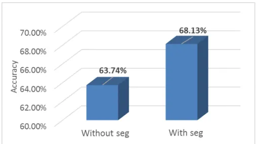
The first thing we want to show is the importance of including segmentation labels in the confabulation model. In this experiment, all knowledge links have the equal weight. We compare the recall accuracy of confabulation models with and without segmentation labels. The result is shown in Figure 2.3. As we can see, adding segmentation label improves recall accuracy by 4.4%.
Another experiment compares the training time, recall time and accuracy be-tween non-circular model and circular model. Table 2.2 shows that non-circular model takes about four times training effort more than the circular model, and 17.5% more recall time, but gives 13% lower recall accuracy.
Table 2.2: Comparison of non-circular and circular model.
Non-circular
Circular
Improvement(%)
Training time(s)
489,180
144,540
70.45%
Recall time(s)
6,317.22
5,207.83
17.56%
accuracy
54.95%
68.13%
13.18%
2.4.2
Analysis of mutual information
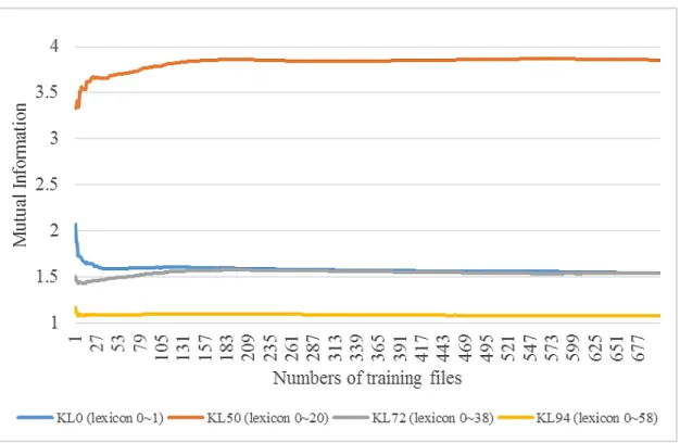
In the second set of experiments, we demonstrate how the change of mutual information (MI) relates to the effectiveness of the training process. We con-tinuously monitor the mutual information of each KL as the training process progresses. The 1328 files of the training corpus is processed one by one. The MI of each KL is calculated each time after a training file is processed.
The line chart in Figure 2.4 shows the change of MI for four selected KLs as the number of processed training files increases. The blue line gives the MI of KL0, which connects two word lexicons of immediate neighbor. We can see that as more files are trained; the MI of KL0 gets smaller. The grey and yellow lines in the figure give the MI of KL72 and KL94 respectively. They are the knowledge links between a single word lexicon and its corresponding tag lexicon. The MI of these KLs fluctuate within a very small range at the beginning of training. When more training files are processed, they converge to a stable value. This is because every Chinese character has its specific semantic and syntactic function and the relation between tags (or segmentation labels) and words are relatively fixed. Very few new character-tag or character-segment relationship will be learned after certain amount of training. In other words, the knowledge base becomes saturated at certain point.
lex-Figure 2.4: Mutual information trend chart for 4 kinds of Knowledge Links. icon and its corresponding word triplet lexicon. Our results show that there is a strong correlation between a word and its corresponding word triplet. This means a character always co-occur with a limited number of word triplets. Sim-ilar to the MI of KL0, 72 and 94, when more training files are processed, the MI of KL50 increases and then gradually saturates to a stable value.
The convergence of MI of KLs indicates that adding more training files will not necessarily increase the learned knowledge. At certain point, the knowledge acquiring speed slows down and further learning will not be as effective as before. It is the time that we should either stop the training or switch to another set of training text that has significantly different style.
Our experimental data show that most Knowledge Links’ mutual
Figure 2.5: Recall accuracy of different training set size.
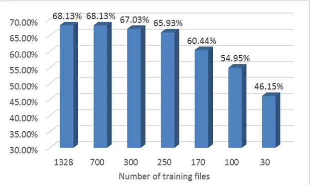
30 and 100 files respectively. We take the knowledge base generated at different stages of training and apply them to sentence completion test. Their recall accu-racy is given in Figure 2.5. The X-axis gives the number of training files used to generate the knowledge base and the Y-axis give the recall accuracy. The graph shows that when training set size exceeds 300, the recall accuracy has stabilized at around 68%, and when the training set size reaches 170, the recall accuracy is already close to its peak. However, if the training set size is too small, the recall quality is not acceptable. This result agrees with Figure 2.4, which shows that the MI of knowledge links starts to converge after 170 training files and becomes very stable after 300 training files. Based on the above discovery, we set the sat-uration threshold of the training set size at 300. Our previous work [101] shows that the training time is linearly proportional to the size of training data. Limit-ing the trainLimit-ing set size to the saturation threshold can sharply reduce trainLimit-ing time with very little sacrifice of accuracy.
Figure 2.6: Knowledge Links’ mutual information.
2.4.3
Quantified Knowledge Link Weighting scheme
The goal of next experiment is to find a systematic way to assign KL weight. Previous works [132] have shown that weighing the contribution of KLs based on their significance can improve recall accuracy, however, their weight is as-signed only in an ad-hoc way. We believe that the significance of a KL can be measured by the mutual information between its source and target lexicons and therefore the MI of a KL should decide its weight.
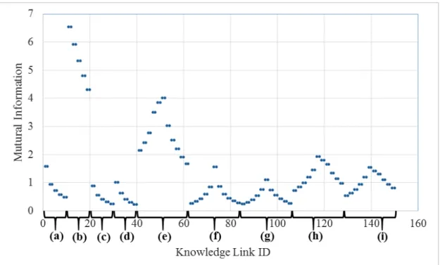
Figure 2.6 shows the mutual information of all knowledge links. Based on their connections, the KLs are divided into 9 groups. The group division is described in Table 2.3. and labeled in Figure 2.6 underneath the X-axis.
We can see from Figure 2.6 that, from left to right, the MI of the KLs in the same group are clustered together. And as the distance between the source and
Table 2.3: Knowledge link grouping.
KL group KL IDs Connection
(a) 0∼9 Between word lexicons
(b) 10∼19 Between word triplet lexicons
(c) 20∼29 Between tag lexicons
(d) 30∼39 Between segmentation label lexicons
(e) 40∼61 Between word and word triplet lexicons
(f) 62∼83 Between word and tag lexicons
(g) 84∼105 Between word and segmentation label lexicons
(h) 106∼127 Between word triplet and tag lexicons
(i) 128∼149 Between word triplet and segmentation label lexicons
target lexicon of the KL increases, the MI of the KL decreases. For example, KL0 and KL8 belong to the same group, therefore, they have similar MI. However, since KL0 connects between two immediate neighboring lexicons while KL8 connects between two word lexicons that are 4 words apart from each other, the MI of KL0 is slightly greater than KL8. This agrees with our intuitions that adjacent characters have stronger correlations. Second, the KLs connecting to word triplet lexicons always give more information than others, therefore they should be weighed as the biggest during the recall.
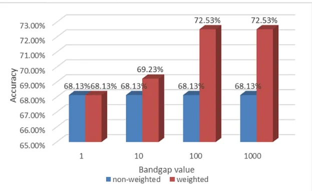
We assign the weight of a KL as a linear function of its mutual information. We then compare the recall accuracy of confabulation models with and without weighted KL. Figure 2.7 shows the recall accuracy of the two sets of confabula-tion models. For each set of models, the Bandgap is varied from 1 to 1000. As we can see, when bandgap value is 10 or less, assigning weight to KL provides little improvement. However, when the bandgap value exceeds 100, assigning weight to KLs brings visible benefits; it improves accuracy by more than 4%. We also observe that, without weighted KL, changing the bandgap value has almost no impact on the recall accuracy. However, with weighted KL, increas-ing the bandgap value from 1 to 10 and 100 can increase recall accuracy from
Figure 2.7