W
W
OR
O
RK
KI
IN
N
G
G
P
P
AP
A
PE
ER
R
NO
N
O
.
.
1
1
5
5
0
0
A Direct Test of the Buffer-Stock Model of Saving
Tullio Jappelli, Mario Padula, and Luigi Pistaferri
December 2005
University of Naples Federico II University of Salerno Bocconi University, Milan CSEF - Centre for Studies in Economics and Finance–UNIVERSITY OF SALERNO
W
W
O
O
R
R
K
K
I
I
N
N
G
G
P
P
A
A
P
P
E
E
R
R
N
N
O
O
.
.
1
1
5
5
0
0
A Direct Test of the Buffer-Stock Model of Saving
Tullio Jappelli
♥, Mario Padula
♠, and Luigi Pistaferri
♦Abstract
Recent models with liquidity constraints and impatience emphasize that consumers use savings to buffer income fluctuations. When wealth is below an optimal target, consumers try to increase their buffer stock of wealth by saving more, while, if wealth is above target, they increase consumption. This important implication of the buffer stock model of saving has not been subject to direct empirical testing. We derive from the model an appropriate theoretical restriction and test it using data on working-age individuals drawn from the 2002 Italian Survey of Household Income and Wealth. One of the most appealing features of the survey is that respondents report the amount of wealth held for precautionary purposes, which we interpret as target wealth in a buffer stock model. The test results do not support buffer stock behavior, even among population groups that are more likely, a priori, to display such behavior. The saving behavior of young households is instead consistent with models in which impatience, relative to prudence, is not as high as in buffer stock models.
Acknowledgements: We thank Chris Carroll for extensive discussions and suggestions and, for comments, Erich Battistin, Annamaria Lusardi, Jon Skinner, Steve Pischke, and seminar participants at the 2005 NBER Summer Institute, the 7th Workshop of the RTN Project on Economics of Aging in Venice, the University of Padua, and the University of Reading. Work supported in part by the European Community’s Human Potential Programme under contract HPRN-CT-2002-00235 [AGE: The Economics of Aging in Europe] and by the Italian Ministry of Education (MIUR).
♥
University of Salerno, CSEF and CEPR ♠
University of Salerno and CSEF ♦
Contents
1. Introduction
2. Deriving testable implications of buffer stock behavior
2.1. Test interpretation
2.2. The simulated covariance ratio 3. Data
4. Testing the buffer stock model 4.1. Baseline estimates 4.2. Group estimates 4.3. Impatience
4.4. Measurement error
4.5. Further sensitivity checks
5. The wealth-income ratio of young households 6. Conclusions
References Appendix
1
Introduction
Recent intertemporal consumption models with impatient individuals emphasize the role of savings as a buffer stock against income fluctuations. Deaton (1991) and Carroll (1992, 1997) have solved sophisticated versions of such models. Although the specific details of the models differ, emphasizing liquidity constraints or the prob-ability of low income realizations, they share similar predictions. In both models, consumers have a unique and stable wealth to permanent income ratio (what we term the target wealth-income ratio). This implies that people who have received negative income shocks, and whose wealth is consequently below target, intend to be “savers”, and thus increase their stock of wealth. People who have received pos-itive shocks, and whose wealth is therefore above target, intend to be “dissavers”, increasing current consumption and running down their stock of wealth.
This key implication of the buffer-stock saving model has not been subject to empirical scrutiny because target wealth is unobservable. Current evidence of buffer-stock behavior is based on two model’s implications: that consumption tracks income closely, and that precautionary saving represents an important reason for wealth accu-mulation. Several simulations of intertemporal consumption models predict consumption-income tracking in the early part of the life-cycle (Attanasio, Banks, Meghir, and Weber, 1999; Laibson, Repetto and Tobacman, 1998; Gourinchas and Parker, 2002; Cagetti, 2003). Empirical evidence on the importance of precautionary saving is mostly based on reduced form regressions of net worth or financial assets on proxies for income risk. Some studies report that precautionary wealth represents a small portion of total wealth, e.g. Guiso, Jappelli and Terlizzese (1992), and Hurst, Ken-nickel, Lusardi and Torralba (2005); othersfind a large impact of income risk, Carroll and Samwick (1997), and Gruber and Yelowitz (1999). These studies differ in many respects, such as the definition of wealth, the measure of risk, and institutional fea-tures. But even findings of large effects of income risk on saving are not conclusive evidence of buffer stock behavior, because life-cycle models with income risk also pro-vide an important role for precautionary saving, see Hubbard, Skinner, and Zeldes
(1995). In short, the literature still lacks a convincing test of the buffer-stock model. In this paper we use a survey question on precautionary wealth available in the 2002 Bank of Italy Survey on Household Income and Wealth (SHIW) to propose a direct test of buffer stock behavior. The question asks people how much savings they think they need for future emergencies, and is similar to a question contained in the 1995 and 1998 Surveys of Consumer Finances described in Kennickell and Lusardi (2004). We interpret this question as providing information on target wealth in a buffer-stock model, and test the proposition that people with wealth-income ratio below target expect to save, while those with wealth-income ratio above target expect to dissave.
We show that the main testable implication of the buffer stock model is that the covariance between the wealth gap (the difference between actual and target wealth) and consumption is (strongly) positive. Although we focus on Carroll’s version of the buffer stock model, the test applies equally well to Deaton’s case. In Carroll, buffer stock behavior emerges from the tension between impatience, prudence, and the chance of zero earnings. Impatient individuals would like to anticipate consumption, but the chance of zero future earnings generates a demand for wealth. In Deaton, the tension is between impatience, prudence, and liquidity constraints, but the insights are similar, and buffer stock behavior emerges again as the optimal policy.
Realistic versions of the buffer stock model with finite horizons and declining in-come after retirement limit considerably the age-range of buffer stock behavior. Car-roll (1997) shows that buffer stock behavior emerges until roughly age 50, and that afterwards people start to accumulate wealth steadily to prepare for retirement. Other models of intertemporal choice deliver different predictions about the correlation be-tween income and consumption and the age-wealth profile during the life-cycle. In the standard life-cycle model without uncertainty, the individual wealth-income ratio is not stationary because consumers save each year until retirement. Hubbard, Skinner and Zeldes (1995) use numerical methods to analyze the properties of a more sophisti-cated life-cycle model with life uncertainty and income risk; their simulations report,
on average, substantial accumulation even at young age. Laibson, Repetto and To-bacman (1998), Attanasio, Banks, Meghir, and Weber (1999), Gourinchas and Parker (2002) and Cagetti (2003) provide structural estimates of stochastic dynamic models of consumption, matching theoretical and observed statistics for US households, and
find a close association between income and consumption in the early part of the life-cycle, and therefore little wealth accumulation at young age, and more substantial wealth accumulation near retirement age. The final part of the paper therefore uses estimates of the age-wealth profile obtained with Italian repeated cross-sectional data to strike a balance between buffer-stock and life-cycle saving behavior.
The rest of the paper is organized as follows. Section 2 reviews the buffer stock saving model, presents the empirical test, based on the stationarity of the target wealth-to-income ratio, and computes the test statistics on data simulated from a re-alistic parametrization of the model. Section 3 describes the survey question on target wealth, and compares it with a similar question asked in the Survey of Consumer Fi-nances. Section 4 presents the test results. Ourfindings suggest absence of significant correlation between the wealth gap and consumption and are thus not consistent with the buffer stock model, regardless of the particular definition of wealth used (real or
financial). We then explore if buffer-stock saving emerges in some population groups that, a priori, are expected to follow buffer stock behavior (the self-employed, the young, and those who face higher income risk). We also split the sample using direct information on the individual rate of time preference available in the 2000 SHIW, which can be merged with the panel section of the 2002 SHIW. Finally, we check the robustness of the test when consumption, cash-on-hand, and target wealth are measured with error. Section 5 uses as organizing framework estimates of the age
pro-file of the wealth-income ratio to explore further if the buffer stock model is able to explain the saving decisions of young households. Section 6 summarizes our findings.
2
Deriving testable implications of bu
ff
er stock
be-havior
We take as our point of departure Carroll’s (1992) buffer-stock saving model to de-rive testable predictions and explain our empirical strategy. Consumers have finite horizons and choose consumption to maximize the following objective function:
E0
T
X
t=0
βtu(Ct)
whereβ is the subjective discount factor, the instantaneous utility function is isoelas-tic, u(Ct) = C
1−ρ
t /(1−ρ), andρ > 0 is the coefficient of relative risk aversion. The
dynamic budget constraint is:
Wt+1 =R[Wt−Ct+Yt]
where R = 1 +r is the constant interest rate factor, and Wt, Yt, andCt are,
respec-tively, non-human wealth, labor income, and consumption at time t . Labor income shifts due to transitory and permanent shocks, both assumed to be log-normally distributed, i.e.,
Yt+1 = Pt+1Vt+1 Pt+1 = GPtNt+1
where Gis the growth rate of income, Pt+1 is permanent income, and Vt+1 andNt+1
are i.i.d. shocks with mean equal to 1. The model also assumes that in each period there is a small chance p > 0 that transitory income is zero. The Bellman equation of the problem is:
Vt(Wt, Pt) = max Ct {
u(Ct) +βEtVt+1(Wt+1, Pt+1)} (1) s.t. Pt+1 =GPtNt+1
To exploit the homogeneity of the instantaneous utility function, let’s define cash-on-hand, Xt, as non-human wealth plus income (Xt=Wt+Yt), and write (1) as:
vt(xt) = max ct { u(ct) +βEtG1−ρNt1+1−ρvt+1(xt+1)} (2) s.t. xt+1 = R[xt−ct] 1 GNt+1 +Vt+1 (3) where xt= WtP+tYt, ct= CPtt andvt(xt) =Vt(Wt, Yt)/Pt1−ρ.
Carroll (2004) shows that for specific ranges of parameter values, the problem has a solution (i.e., the functional defined in 2 has afixed point), optimal consumption is an increasing and concave function of cash-on-hand, and the marginal propensity to consume out of cash-on-hand is bounded from above and from below. Furthermore, there exists a unique and stable cash-on-hand-to-permanent income ratiox∗such that, “if actual cash-on-hand is greater than the target, impatience will outweigh prudence, and wealth will fall, while if cash-on-hand is below the target, the precautionary saving motive will outweigh impatience and the consumer will try to build wealth back up toward to target” (Carroll, 2001, p. 33).1 In our notation, if (x
t−x∗)<0,
then the cash-on-hand to permanent income ratio grows in expectation. If instead
(xt−x∗)>0,xt falls (again, in expectation). Using cross-sectional data, we test this
key implication of the model.
At any given point in time, households differ in their value of the wealth gap
(xt−x∗). Afirst source of heterogeneity concerns preferences and the parameters of
the income generating process, which set different values of x∗ for each individual.
Income shocks are a second source of heterogeneity: even if two identical consumers have the same preferences and the same income generating process - and therefore the samex∗ - they receive different income shocks and have therefore differentx
t and
wealth gaps.2
1Carroll (2004) shows also that, at the target, expected consumption growth is less than expected permanent income growth; and that expected consumption growth is declining in cash-on-hand.
2These are not the only possible sources of heterogeneity. In Section 2.2 we use simulation analysis to explore the effect of heterogeneity in income risk, income growth, and interest rates.
Thus in a cross-section, the implication we test is that:
COV(xht−x∗h, Eht(xht+1−xht))<0 (4)
whereCOV (., .)is a population covariance andhis a household index. This notation makes explicit that Eht(xht+1−xht) is the time t expectation of household h’s next
period change in cash-on-hand, and the covariance is taken with respect to the cross-sectional distribution of the wealth gap and of expected asset accumulation.
To test this restriction one needs to observe x∗
h, xht and Eht(xht+1). As we shall
see, we have data on actual wealth and on a proxy of target wealth, but not on the expected value of the change in cash-on-hand. To evaluate Eht(xt+1), let’s take
the expectation as of time t of (3) for household h, and recall that Eht(Nt+1) = 1, Eht(Vt+1) = 1, andV ARht(lnNt+1) =σ2N: Eht(xht+1) = R[xht−cht]∗Eht µ 1 GNt+1 ¶ +EhtVht+1 ≈ RG[xht−cht]∗eσ 2 N + 1 (5)
where the second equality follows from a second order Taylor expansion of 1
Nht+1around
the mean of Nht+1.
Substituting (5) in (4) and defining γ = eσ2
N, we can restate (4) in terms of
observable variables as:3
θ = COV(xht−x ∗ h, cht) COV(xht−x∗h, xht) > µ 1− G Rγ ¶ (6) The right-hand-side of the inequality (6) is positive, becauseσN >0impliesγ >1,
while the condition G < R guarantees a finite present discounted value of income. According to the model, the left-hand-side should therefore be positive. Intuitively, people above target have a relatively high consumption to permanent income ratio (and vice versa). As we shall see below, the proposed test has a simple instrumental-variable interpretation, which delivers further interesting insights.
3Equation (6) is the relevant condition only ifCOV(x
ht−x∗h, xht)>0. Since this is what holds
2.1
Test interpretation
Dropping the time subscripts, the sample analog of the left-hand-side of the inequality (6) is: bθ= cov(xh−x ∗ h, ch) cov(xh−x∗h, xh) = PH h=1((xh−x∗h)−(xh−x∗h)) (ch−ch) PH h=1((xh−x∗h)−(xh−x∗h)) (xh−xh)
where cov(., .) is a sample covariance and a bar over a variable denotes its cross-sectional mean. The same expression can be obtained from an (exactly identified) IV regression of ch on xh using (xh −x∗h) as an instrument. This suggests running the
following regression:
ch =η+θxh+uh (7)
using the wealth gap as an instrument for x, and testing the null hypothesis that θ,
which from now on we term the covariance ratio, equals zero. Afinding thatθ ≤0is unambiguously inconsistent with the buffer stock model. But θ >0 might still reject the model if θ < ³1−RγG´. Thus it is useful to have an idea of how large the term
³
1−RγG´is.
Consider first the case G = 1 (no productivity growth), and note that in the absence of uncertainty (σ2
N = 0, orγ = 1), or in models with quadratic preferences in
which consumers do not react to uncertainty, the marginal propensity to consume out of wealth is just the annuity value, or lim
σ2
N→0
³
1−Rγ1 ´= 1+rr.4 As income uncertainty increases, the MPC reaches an upper value of one, lim
σ2 N→∞ ³ 1−Rγ1 ´ = 1. Allowing for productivity growth (G >1) has the opposite effect, because an increase inGreduces the MPC.
To provide realistic and operative bounds for the test and the value of the marginal propensity to consume, one needs specific values for the model parameters. Carroll (2001) proposes an interest rate equal to 4 percent per year, 3 percent productivity growth rate, and a standard deviation of permanent income shocks of 0.10,
sponding to³1−RγG´= 0.019. Parameters for the Italian economy provide a slightly higher value. On average, in the past two decades the productivity growth rates of Italian workers in the age group (20-50) has been 1.5 percent per year. Jappelli and Pistaferri (2006) estimate with panel data that the standard deviation of per-manent income shocks is 0.16. Assuming that the interest rate is 2.5 percent, raises the reference wealth coefficient in equation (7) to 3.6 percent. Therefore, values of the estimated covariance ratiobθ ≥ 0.036 are potentially consistent with buffer stock behavior.
2.2
The simulated covariance ratio
The empirical test of the previous section compares the estimated covariance ratiobθ
with the lower bound of the distribution of θ under the hypothesis that the model is true. However, to have a better grasp of the empirical results, one should be able to answer the question: How large should θ be in a buffer stock model? This value depends on the specific assumptions one makes about the parameters of the model and it might be very far from the lower bound derived above.
To answer this question, we simulate the model for an economy populated by heterogeneous consumers, compute the wealth gap for each, and compute the cross-sectional covariance ratio θ. In the baseline simulation, we assume that the interest rate is 2.5 percent, the growth rate of permanent income 1.5 percent, the probability of zero income 0.5 percent, and the coefficient of relative risk aversion 2. Permanent and transitory income shocks are drawn from lognormal distributions with mean equal to 1 and standard deviation equal to 0.16 and 0.28, respectively (Jappelli and Pistaferri, 2006). Consumers differ because the discount factor is uniformly distributed between 0.86 and 0.96, and because, at any given point in time, they are hit by different income shocks. We further assume that consumers start with zero wealth.
The optimal consumption function is a structural relation between the ratio of consumption to permanent income and the ratio of cash-on-hand and permanent in-come. As shown in Carroll (2004), the function is bounded from below and from
above, and so is its derivative. Moreover, it is increasing and concave. The con-sumption function is usually found by solving the model numerically. Here, instead, we use an approximate consumption function:
ct = 2(κ−κ){xt−
1
b[log(1 + exp(bxt))−log(2)]}+κxt
where
κ = 1−R−1(Rβ)1ρ
κ = 1−R−1(pRβ)1ρ
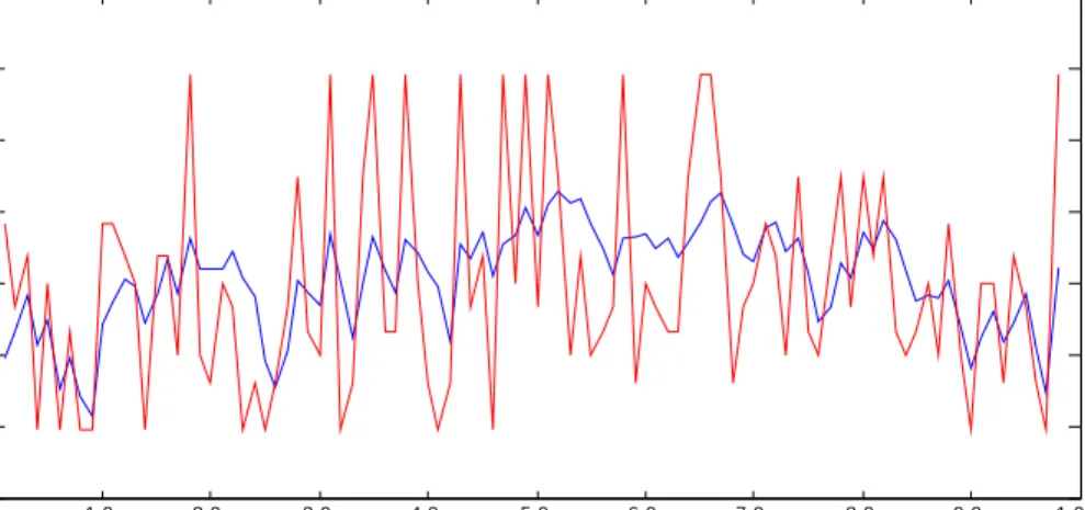
and R, β, ρ, and p are defined in Section 2 and b= 1.02. Carroll (2004) derives the expressions of κ andκ, while Padula (2005) proposes this approximate consumption function and documents its properties. For the baseline case, the correlation coeffi-cient between the numerical solution and the analytical approximation is 0.96, and is robust to a wide range of admissible parameter values. Figure 1 plots income and consumption to permanent income ratios for a typical consumer. The figure shows that consumption is smoother than income, and that large income shocks produce less pronounced consumption changes, as in standard buffer stock models.
Using the analytical approximation and the budget constraint, and assuming that consumers start with zero wealth, we simulate the model for 100 periods and 1,000 consumers. We then compute, for each consumer, target wealth as the ratio between cash-on-hand and permanent income such that Etxt+1 =xt. To calculate θ we
com-pute the covariance ratios at each point in time and then average them across the 100 periods. For the baseline experiment we findθ = 0.3995, an order of magnitude larger than the 0.036 lower bound obtained for the same set of parameter values. This value is remarkably close to the covariance ratio computed solving the model numerically (θ = 0.3965), which we interpret as further confirmation of the validity of the approximate consumption function.
We also compute the covariance ratio under very different assumptions about the source of heterogeneity in the model. We allow for heterogeneity in the growth
rate of income, interest rate, permanent income shocks (and various combinations of heterogeneity sources), and find that the covariance ranges from 0.20 to 0.43.5
Overall, the simulation results suggest that realistic values of the covariance ratios lie much above the theoretical threshold.
3
Data
To implement the empirical test of the buffer stock model, we use the 2002 Italian Survey of Household Income and Wealth (SHIW), a biannual representative sample of the Italian population conducted by the Bank of Italy.6 The sample includes about
8,000 households and 24,000 individuals. Details on questionnaire, sample design, response rates, results and comparison of survey data with macroeconomic data are given in Biancotti et al. (2004).
For our purposes, the SHIW has several advantages. It has data on wealth, in-come, consumption, and detailed demographic characteristics of the household. Net
financial assets measure the liquid portion of wealth, and are the sum of transaction accounts, government bonds, CDs, corporate bonds, retirement accounts, life insur-ance, and stocks, less household debt (mortgage loans, consumer credit and other personal loans). Total assets are the sum of netfinancial assets and real assets (real estate, unincorporated business holdings, valuables and art objects). The SHIW also includes a rotating panel component: 45 percent of the households interviewed in 2002 were also interviewed two years before. We will later use the panel section of the SHIW to recover individual-level variables available only in the 2000 survey.
Most importantly for the present study, the 2002 SHIW has a direct question
5We consider cases in which the growth rates of income are uniformly distributed between 1 and 2 percent, interest rates between 2 to 3 percent, and standard deviation of permanent income shocks between 10 to 20 percent. All these results are available on request.
6In the buffer stock model, the marginal propensity to consume is high because consumers are impatient. Carroll (2001) interprets the excess sensitivity of consumption found by Campbell and Mankiw (1991) and Jappelli and Pagano (1989) in time series data for several OECD countries, and in Italy in particular, as dependent on the prevalence of impatient households. He argues that in these countries there are “more households who are impatient and consequently inhabit the portion of the consumption function where the MPC is high, whether they are formally constrained or not” (Carroll, 2001). Italy, therefore, provides a good testing ground for the buffer-stock model.
on precautionary wealth, which we use to proxy target wealth in the buffer stock model: “People save in various ways (depositing money in a bank account, buying
financial assets, property, or other assets) and for different reasons. Afirst reason is to prepare for a planned event, such as the purchase of a house, children’s education, etc. Another reason is to protect against contingencies, such as uncertainty about future earnings or unexpected outlays (owing to health problems or other emergencies). About how much do you think you and your family need to have in savings to meet such unexpected events?” The question is patterned after a similar question in the Survey of Consumer Finances (SCF), described in Kennickell and Lusardi (2004).7
Table 1 reports sample means and quartiles of target wealth for various sample groups. The median value of target wealth is euro 25,000, and the mean is euro 49,990. Interestingly, these values are higher than in the U.S., where Kennickell and Lusardi (2004) report that the bulk of the distribution of target wealth is between $5,000 and $10,000. Target wealth is higher among high-school and college graduates, self-employed, households with multiple income recipients, and households living in the North. Descriptive analysis shows that the distribution of target wealth mirrors that of cash-on-hand, consistent with thefindings reported in Kennickell and Lusardi (2004) for the U.S.
The median ratio of target wealth to total wealth is 0.27, and 2.5 if wealth includes onlyfinancial assets. These numbers are higher than in Kennickell and Lusardi (2004) - 0.08 and 0.2 respectively. This shows that in Italy precautionary wealth potentially accounts for a larger portion of wealth, possibly due to higher income risk and/or lower degree of development of financial and insurance markets. The Italian data also indicate that in 70 percent of the casesfinancial wealth is below target, and in 27 percent of cases real wealth is below target. Comparable figures for Kennickell and Lusardi (2004) are 48 and 17 percent, respectively.
7The SCF question is: “About how much do you think you and your family need to have in savings for unanticipated emergencies and other unexpected things that may come up?”. As in the SCF, the question is asked in the wealth and saving section of the questionnaire. The question has been extensively tested in the SCF with focus groups.
In the empirical application we measure consumption as non durable expendi-tures.8 We define cash-on-hand as Y +W
f +λWr, where Y is household
dispos-able income, Wf and Wr are, respectively, net financial assets and real assets, and
0≤λ≤1 measures the portion of real assets that can be used in the current period to finance consumption. We focus on a sample where buffer stock behavior is more likely to emerge, selecting household with heads between 20 and 50 years old. The resulting sample consists of 2,953 observations.
In keeping with the model’s notation, consumption, target wealth, cash-on-hand and the wealth gap are all normalized by an estimate of permanent income, that is, income during the working life purged from transitory components. The permanent component of income is estimated by thefitted value of a regression of household
non-financial income on age, education, dummies for occupation, region of residence, head gender and number of earners in the household. We experiment with other regressions (for instance, using other sample years, other variables, or interaction terms) andfind that the test results are qualitatively unchanged. We therefore opt for a simple and straightforward definition. In Section 4.5 we adopt a different strategy, relying on time-averages of income obtained using the panel component of the survey. The advantage is that this measure is potentially closer to the income stochastic process assumed in Section 2. The drawback is that the number of observations is considerable reduced. In practice, the results appear to be very similar.
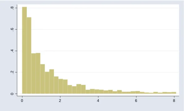
Figure 2 plots the histogram of the ratio of target wealth to permanent income. Median target wealth represents slightly less than one year of income, and the bulk of the distribution is between 3 months and two years. Table 2 reports sample statistics for various population groups. The ratio of target wealth to permanent income is higher for single earners and resident in the North, but overall it is quite stable across different population groups.
8Results are unchanged if one defines consumption as the sum of non durable and durable ex-penditures, see Section 4.5.
4
Testing the bu
ff
er stock model
In this section we estimate the covariance ratio θ. The previous section shows that realistic values of the parameters of the buffer stock model deliver values of θ of at least 3.6percent. Simulation analysis with the same parameter values, suggests that
θ in practice is around 30percent. After presenting full sample estimates, we test if
θ is higher among households that face higher income risk and are therefore expected to exhibit stronger buffer stock behavior. A related issue is that both Deaton’s and Carroll’s models apply to impatient consumers. Using a direct survey question, we are able to split the sample by high and low rates of time preference. If one or more of the relevant variables are measured with error, estimation of (7) provides incorrect inference. For instance, ifxh is measured with error, using(xh−x∗h)as an instrument
delivers a downward biased estimate of the true θ.9 After presenting our baseline
results and the group estimates, we therefore check robustness to measurement error. Finally, we check the sensitivity of the estimated covariance ratio using different definitions of income and consumption.
4.1
Baseline estimates
The first row of Table 3 displays baseline estimates for the whole sample, obtained regressing consumption on cash-on-hand, and using the wealth gap as instrument. In the first column, we set λ = 1 and cash-on-hand is just Y +Wf +Wr, on the
assumption that households can use all assets to buffer income shocks. The point estimate of θ is positive, as predicted by the buffer stock model. However, the size of the coefficient (0.011) is too small to be consistent with the model. And since the estimate has a small standard error, we formally reject the hypothesisθ = 0.036 (the lower bound of θ under the null of the buffer-stock model), let alone the hypothesis that θ equals one of the simulated values of Section 2.2. In the other columns we use different definitions of wealth, obtained setting λ = {0.75,0.50,0.25}, because transaction costs, illiquidity, and indivisibilities may allow consumers to use only a
9Apart from the unlikely case in which measurement errors inx
portion of their real assets as a buffer. Wefind thatbθ ranges from 1.2 to 1.5 percent, never exceeding the buffer stock lowest threshold and therefore failing to support the model.
4.2
Group estimates
Even if our baseline results do not support it, the buffer-stock model might still characterize the behavior of some population groups that face high income volatility or are more impatient. We are particularly interested in testing the buffer-stock behavior for groups that, a priori or based on previous evidence, are more likely to exhibit such behavior. The self-employed clearly face greater income risk than employees. If the incomes of households with multiple earners are not perfectly correlated, single income households face more risk than households where both spouses work. The young might face more income uncertainty, or be more impatient than the middle-aged because they don’t yet perceive the need to accumulate for old age. In Italian regions with better functioning credit and insurance markets (the North and the Centre), employment shocks and other risks are more likely to be insured. And in the case of education, we have hard evidence with the same dataset that the two groups face different income risks.
To check if buffer stock behavior characterizes some population groups, in Ta-ble 3 we present estimates of θ distinguishing between relatively younger and older households (age less or greater 40), single and multiple earners, employees and self-employed, and region of residence. In the first column bθ never exceeds 1.5 percent, confirming the full sample estimates for each of the group considered. Interestingly, the pattern of coefficients is at variance with priori hypotheses on buffer stock be-havior. The estimated coefficient is lower among the young, the self-employed and single earners, and in each case the coefficients are precisely estimated and we can therefore reject the hypothesis that they are equal in the two groups. The estimates for different definitions of cash-on-hand do not change the pattern of results.
busi-ness owners. Busibusi-ness owners and entrepreneurs face higher income risk, but their wealth holdings are also higher than average. Hurst et al. (2005) provide evidence that tests of precautionary saving are considerably affected by the treatment of en-trepreneurs. In the total sample, theyfind a strong, positive relation between wealth and permanent income shocks, as in Carroll and Samwick (1987). But the result is almost entirely due to business owners: when these are excluded from the sample, there is hardly evidence for precautionary saving. Table 3 reports bθ distinguishing by entrepreneurship, defined as positive business wealth. The results are again at variance with the buffer stock model for both groups, as bθ is uniformly lower than the threshold value for business owners and non-owners. However, in this case the relative size of the coefficients agrees with expectations, as bθ is generally higher for business wealth owners (except when λ= 1).
Comparison of different population groups with different income generating process is quite interesting, because in this case we can rely on our previous work using Ital-ian microeconomic data to estimate the same income process postulated in the buffer stock model and specified in Section 2. Jappelli and Pistaferri (2006) estimate that the variance of permanent income shocks is 0.0296 for the less well educated, and
0.0198 for those with at least a high school degree. Carroll and Samwick (1997), us-ing U.S. data, alsofind that the less well educated face a higher variance of permanent income shocks. Setting the interest rate at 2.5 percent, the growth rate of earnings at 1.5 percent and using these group estimates for income volatility, the threshold
(1−RγG) is 3.9 percent for the less well educated and 2.9 percent for households with higher education. This implies that one should find a higherbθ in the first group.
The results in Table 4 do not support this hypothesis: in the first column, bθ is 1 percent in the group with lower education, and 1.3 percent in that with higher education. The results are similar for the other definitions of cash-on-hand: the data do not speak in favor of the buffer stock model.
4.3
Impatience
The rate of time preference is a critical parameter of models of intertemporal choice, but microeconomic data seldom allow to pin down particular features of this and other preference parameters. The 2000 SHIW attempts at providing data on time prefer-ence through a lottery question. Frederick, Loewenstein, and O’Donoghue (2002) survey theoretical and empirical research on time preferences, and classify the vari-ous methods by elicitation methodology (choice, matching, rating or pricing), type of instrument used to elicit preferences (field versus experiment), and time frame (less than one day to many years). They report that a widely used way to elicit the rate of time preference is through survey questions asking the respondent to report how much he or she is willing the pay to receive a lottery winnings today instead of later in time. The 2000 SHIW has precisely such question: “Suppose that you win euro 5,000, payable for certain in a year’s time. What is the maximum amount that you are willing to pay to have the euro 5,000 immediately?”.
The question is asked only to half of the sample (household heads born in odd-numbered years), and about 15 percent don’t answer. The 2000 data can be merged with 2002 data using the panel component of SHIW (45 percent of the sample). After merging the data, and considering that in 2002 we focus only on people less than 50 years old, we are left with 498 valid observations with data on both target wealth and time preference. On average, to cash the lottery one year in advance, respondents are willing to pay 300,000 lire (about 150 euro), implying a quite standard rate of time preference of 3 percent a year. Several studies use questions similar to this, as documented in Frederick, Loewenstein, and O’Donoghue (2002), who also reviews pros and cons of various methods for eliciting time preference.10
We therefore split the sample according to whether the rate of time preference is above or below 3 percent. Table 5 reports the estimatedθ in the two sub-samples. It is important to keep in mind that the sample in this case is highly selected, and that
10Frederick, Loewenstein, and O’Donoghue (2002) emphasize that measurement of time preference can be affected by confounding factors, such as uncertainty, intertemporal arbitrage and consumption smoothing.
we have relatively few observations. Buffer stock behavior is rejected in both groups, asbθ ranges between 1.3 and 1.9 percent. Interestingly, thebθ for the high impatience group is higher for all measures of cash-on-hand (except λ= 0.25).
4.4
Measurement error
To explore the robustness of our findings to the possibility that consumption, cash-on-hand and target wealth are measured with error, it is useful to rewrite (6) as:
θc> θx µ 1− G Rγ ¶ (8) where θc = COV(ch,xh−x∗h)
V AR(xh−x∗h) is the OLS coefficient of the population regression ofch on
xh−x∗h, θx =
COV(xh,xh−x∗h) V AR(xh−x∗h) 6
= 0 the OLS coefficient of the population regression of
xh on xh −x∗h, and the covariance ratio θ = θc θx.
11 Let’s assume that consumption,
cash-on-hand and the target are all measured with error and thus define:
ech = ch+εch
e
xh = xh+εxh
e
x∗h = x∗h+εxh∗
where tilded variables are observed, untilded are true, unobserved values, and εk h is
a measurement error in variable k having mean zero. Under the assumptions that the errors are uncorrelated with each other and with true consumption, cash-on-hand and target wealth, one can show that:
plim H→∞ b θc = θc 1 +ηx+ηx∗ (9) plim H→∞ b θx = θx 1 +ηx+ηx∗ + ηx 1 +ηx+ηx∗ (10) where ηx = V AR(εxh) V AR(xh−x∗h) andη x∗ = V AR(εx ∗ h ) V AR(xh−x∗h).
11We assume in this section thatθ
Measurement error biases downward the OLS coefficient of the regression of con-sumption on wealth-gap (bθc).12 The bias of the OLS coefficient of the regression of
cash-on-hand on target wealth (bθx) might be either negative or positive. Observing
an estimate of the covariance ratio below the threshold³1−RγG ´= 0.036may lead to a false rejection of the buffer-stock model if there is measurement error in the relevant variables. In particular, measurement error modifies condition (6) as follows:
θ > µ 1− G Rγ ¶ − µ 1− G Rγ ¶ V AR(xeh) V AR(xeh)−COV (exh,ex∗h) ξ (11)
where ξ =V AR(εxh)/V AR(exh) is the fraction of the total variance of observed
cash-on-hand due to measurement error (see the Appendix for derivations). Condition (11) shows that even values of the covariance ratio below the threshold ³1−G
Rγ
´
= 0.036
(as, say, those estimated in Table 3) may be consistent with buffer-stock behavior if there is enough measurement error in the variables of interest.13 In other words,
the lower bound of the test (the right-hand side of (11)) declines as the variance of measurement error increases.
Equation (11) can be used to see how large measurement error has to be in order for the model to be true when the data reject it. Figure 3 plots the right-hand side of (11) as a function of ξ. We set ³1−G
Rγ
´
= 0.036 and estimate the variance and covariance terms in (11) from the data. The graph shows that in the absence of measurement error ξ = 0 and the bound is ³1−RγG´ = 0.036 as assumed thus far. For ξ ≥ 0.66 the model is falsely rejected due to measurement error. Thus, if measurement error accounts for at least two-thirds of the observed variability of cash-on-hand, our results are misleading. Since the reliability index of income and wealth in the SHIW exceeds 80 percent (Biancotti et al. 2004), it is unlikely that measurement error invalidates our test.14 The results are similar if one uses different
12Note that¡1 +ηx+ηx∗¢
= V AR(hxh−xh∗h)
V AR(xh−x∗h) >1.
13This requiresV AR(xe
h)−COV (xeh,xe∗h)≥0, i.e., thatxeh covaries with itself at least as much
as withxe∗
h.
14Biancotti, D’Alessio and Neri (2004) give extensive account of the quality of the main variables in SHIW. Exploiting the panel section of the survey, they compute the reliability index for a broad range of variables. The index is the fraction of total variability of the measured characteristic accounted by its true variability.
definitions of wealth or estimates splitting the sample by socioeconomic groups.
4.5
Further sensitivity checks
Our measure of permanent income, which we use to normalize cash-on-hand, con-sumption, and target wealth, is obtained through cross-sectional regressions, and may not be purged from transitory components. In Table 6 we report the estimated co-variance ratio using an alternative measure, obtained averaging household disposable income (net of financial income) over time. This measure can only be computed for households in the 2000-02 panel section of SHIW. Averaging should remove compo-nents that are purely transitory and mean-reverting. The results are similar, although the estimate of θ is less precise due to the reduced number of observations.
So far, our tests have been conducted defining consumption as non-durable expen-diture. SHIW has also data on expenditures on durable goods, and therefore we can use total expenditure as an alternative measure of consumption. As a further sensi-tivity check, we exclude financial income from the definition of income andfind that the results are not affected, as shown in Table 6. The results are our also unchanged if one exclude housing wealth from total wealth.
5
The wealth-income ratio of young households
The version of the buffer stock model that we analyze is one with impatient con-sumers, uncertainty about future earnings, and no borrowing constraints. If such consumers are sufficiently prudent and expect their earnings to grow over time, they will never borrow and keep their consumption within their current incomes, thus in-ducing “tracking” between consumption and income. In other versions of the buffer stock model, impatient consumers would like to borrow but are prevented to do so because of credit market imperfections, as in Deaton (1991). The implications for the behavior of consumption and wealth are similar, however, and “consumption is smoothed, not over the whole life-cycle, but over much shorter periods of a few years at a time” (Deaton, 2005). In the literature, this is often referred to as “high-frequency”smoothing of income, as opposed to the “low-frequency” or “life-cycle frequency” smoothing that was postulated by Modigliani and Brumberg.
Tracking of income and consumption and buffer stock behavior stand in sharp contrast with one of the most important implications of the Life-Cycle Hypothesis, according to which young people save for post-retirement expenditures, and accumu-late wealth up to retirement. In the certainty version the model, the wealth-income ratio increases during the working span, target wealth-income ratio is reached at re-tirement age, and the consumption and income profiles are completely detached. If income is expected to increase over the working life, consumers borrow early in life, and start accumulating wealth only when debt is repaid, which might be even after several years of work, depending on preferences and the growth rate of individual incomes (Hubbard and Judd, 1986).
In a more sophisticated version of the life-cycle model with income risk and life uncertainty, Hubbard, Skinner and Zeldes (1995) show that sufficiently patient con-sumers save even earlier in life. In these life-cycle models with income risk, uncertainty generates a demand for precautionary saving during the working span. But, as noted by Modigliani (1986), accumulated assets can serve the double purpose of providing resources for retirement and a buffer against unexpected emergencies.
Gourinchas and Parker (2002) results fall in between these two polar cases. They estimate that the behavior of young consumers exhibits buffer stock behavior, at least in the U.S. These consumers would like to borrow but cannot, or are too prudent to borrow. One way or another, their consumption tracks income closely and the wealth-income ratio is approximately constant. Once consumers reach middle-age, however, they follow the standard life-cycle model and the wealth-income ratio increases until retirement. Carroll’s (1997) simulations of age profile of the wealth-income ratio is indeed consistent with these findings. Similar tracking of income and consumption arises in models with hyperbolic discounting, see Laibson, Repetto and Tobacman (1998).15 The age profile of the wealth-income ratio of young and middle-aged
sumers provides therefore a useful avenue to distinguish different classes of models of intertemporal choice.
In the previous section we establish that Italian wealth data are at variance with the buffer stock model. Even though we select a sample where buffer stock behavior is most likely to arise (individuals aged 20 to 50, or individuals with relatively high rates of time preference), we do not find evidence that deviations of wealth from target are offset by changes in consumption. What then explains the saving decisions of young households? Here we attempt to discriminate between different saving models providing evidence on the saving behavior of young consumers and estimating their age-wealth profiles.
A single cross-section is not suitable to the purpose of estimating age-profiles, since in a given year age is perfectly collinear with year of birth (Shorrocks, 1975). The individuals interviewed in any cross-section belong to generations that differ in productivity, mortality, preferences, and economic environment. For instance, someone who entered the labor force in the sixties experienced different productivity growth and might have different preferences than an individual born in the eighties and just now entering the labor force. Thus, a finding that the wealth-income ratio increases changes with age in a cross-section may tell very little about households’ behavior.
With panel data or repeated cross-sectional data one, can recover age effects under suitable identification assumptions. Panel data allow the econometrician to track individual wealth trajectories over time. When long panels with wealth data are not available, repeated cross-sectional data can partly overcome their absence. Although the same individual is only observed once, a sample from the same cohort is observed in a later survey, so that one can track the wealth not of the same individual, but of a representative sample of individuals of the same cohort.
We use income and wealth data from seven surveys (1989, 1991, 1993, 1995,
discounting, because hyperbolic consumers hold a smaller share of assets in liquid form, see Angeletos et al. (2001).
1998, 2000 and 2002), a total of almost 60,000 households.16 Income is defined as household disposable income, net of financial income. To account for the fact that some of the wealth is illiquid and cannot be used for precautionary purposes, we use two definitions of wealth, total assets and net financial assets.
We use the repeated cross-sections to sort the data by the year of birth of the head of the household. The first cohort includes all households whose head was born in 1939 (50 years old in 1989, thefirst year of the sample). The second includes those born in 1940, and so on up to the last cohort, which includes those born in 1980 (22 years old in 2002, the last year). As with other survey data, the wealth distribution is skewed. We report only results for the average wealth-income ratio; results for the median ratio are similar and are not reported for brevity.
The left graphs in Figure 4 offers important insights into the process of wealth accumulation of young Italian households. To make the graphs more readable, we plot only the wealth-income ratio and the financial wealth-income ratio of four selected cohorts. The numbers in the graph refer to the year of birth, extending from 50 (individuals born in 1950) to 65 (individuals born in 1965). Except for the youngest and the oldest generations, each cohort is observed at seven different points in times, one for each cross-section. The cross-sections run from 1989 to 2002. Thus, each generation is observed for 13 years with each line being broken (for instance, cohort 60 is sampled 7 times from age 29 in 1989 to age 42 in 2002). Both ratios are potentially affected by age, cohort and time effects.17
To estimate the age profile of the wealth-income ratio, one can proceed as Deaton and Paxson (1994), regressing the wealth-income ratio on age dummies, cohort dum-mies, and restricted year dumdum-mies, summing to zero and orthogonal to a time trend. An alternative identification assumption is to express the ratio as a function of age
16In the SHIW households are defined to include all persons residing in the same dwelling who are related by blood, marriage or adoption. Individuals selected as “partners or other common-law relationships” are also treated as families.
17Two macroeconomic episodes characterize our sample period. The economy went into a recession in 1991-93. Afterwards the economy began a mild recovery, with the growth rate picking up in 2000, and falling in 2002.
dummies and unrestricted time dummies (eliminating cohorts effects). This alter-native decomposition delivers, qualitative similar results, e.g., an increasing wealth-income ratio. Both normalizations rule out time-age or time-cohort interaction terms The wealth-income equation is estimated on 203 age/year/cohort cells. Given the structure of our sample, the regressors include 28 age dummies (from age 22 to age 50), 41 cohort dummies (from 1939 to 1980), a set of restricted time dummies, and a constant term. Under the assumptions described above, the estimated age dummies can be interpreted as an individual age-wealth profile, purged from cohort effects.
The right-hand-side of Figure 4 plots the estimated age dummies, separately for the total wealth and financial wealth-income ratios. Both ratios increase with age. Between age 20 and 50 there is a six-fold increase in the wealth-income ratio (from 1 to 6), and a three-fold increase in thefinancial wealth-income ratio (from 0.4 to 1.2). Since wealth accumulation may depend also on other characteristics (household size and composition, rules governing retirement, education, gender, region of resi-dence) we estimate an extended specification on the repeated cross-.sectional data. We also exclude households with heads less than 30 years old, to account for the fact that young working adults with independent living arrangements tend to be wealthier than average, affecting the age-wealth profile. In both cases the qualitative results of increasing age-wealth profile in Figure 4 is unchanged. Overall, the evidence suggests that models in which consumption and income of young households track each other closely are not an adequate description of the behavior of Italian households. Rather, consumers start saving early in life, and accumulate assets at the rate of around 15 percent of their income, or euro 5,000 euro per year.
6
Conclusions
Intertemporal models with liquidity constraints, income risk, and impatience empha-size that consumers use savings to buffer incomefluctuations. These models deliver a stationary distribution of the ratio of target wealth to permanent income. When actual wealth, relative to income, is below the optimal target, consumers try to
in-crease their saving. When wealth is above target, they inin-crease consumption. This important implication of the buffer stock model has not been subject to direct empir-ical testing. We derive from the model an appropriate theoretempir-ical restriction and test it using data drawn from the 2002 Italian Survey of Household Income and Wealth. One of the most appealing features of the survey is that people report the amount of wealth held for precautionary purposes, which we interpret as target wealth in the buffer stock model. The test results do not support buffer stock behavior, even among population groups that are more likely, a priori, to display such behavior (the young and the self-employed). Measurement error in target wealth or consumption is unlikely to explain the model’s failure. The age-wealth profile of young households provides further indirect evidence against buffer stock behavior.
References
[1] Angeletos, George-Marios, David Laibson, Andrea Repetto, Jeremy Tobacman, and Stephen Weinberg (2001), “The Hyperbolic Consumption Model: Calibra-tion, SimulaCalibra-tion, and Empirical EvaluaCalibra-tion,” Journal of Economic Perspectives
3, 47-68.
[2] Attanasio, Orazio P., James Banks, Costas Meghir, and Guglielmo, Weber (1999), “Humps and Bumps in Lifetime Consumption,”Journal of Business and
Economic Statistics 17, 22-35.
[3] Black, Dan A., Mark C. Berger, and Frank A. Scott (2000), “Bounding Para-meter Estimates with Nonclassical Measurement Error,” Journal of American
Statistical Association 95, 739-748.
[4] Biancotti, Claudia, Giovanni D’Alessio, and Andrea Neri (2004), “Errori di misura nell’indagine sui bilanci delle famiglie italiane,” Temi di discussione, n.520. Rome: Bank of Italy.
[5] Biancotti, Claudia, Giovanni D’Alessio, Ivan Faiella, and Andrea Neri (2004), “I bilanci delle famiglie italinane nell’anno 2002,” Supplementi al Bollettino Statis-tico 14, n. 12. Rome: Bank of Italy.
[6] Brandolini, Andrea, and Luigi Cannari (1994), “Methodological Appendix: The Bank of Italy’s Survey of Household Income and Wealth,” in Saving and the Accumulation of Wealth: Essays on Italian Households and Government Behav-ior, Albert Ando, Luigi Guiso, and Ignazio Visco eds. Cambridge: Cambridge University Press.
[7] Cagetti, Marco (2003), “Wealth Accumulation over the Life Cycle and Precau-tionary Savings,”Journal of Business and Economic Statistics 21, 339—353.
[8] Campbell, John Y., and Gregory Mankiw (1991), “The Response of Consumption to Income: A Cross-Country Investigation,”European Economic Review, 35, 723-767.
[9] Carroll, Christopher D. (1992), “The Buffer-Stock Theory of Saving: Some Macroeconomic Evidence,”Brookings Papers on Economic Activity 1, 61-156. [10] Carroll, Christopher D. (1997), “Buffer-Stock Saving and the Life
Cy-cle/Permanent Income Hypothesis,”Quarterly Journal of Economics 112, 1-56. [11] Carroll, Christopher D. (2001), “A Theory of the Consumption Function, with and without Liquidity Constraints,”Journal of Economic Perspectives 15, 23-45. [12] Carroll, Christopher D. (2004), “Theoretical Foundations of Buffer Stock
Sav-ing,” John Hopkins University, Working Paper n. 517.
[13] Carroll, Christopher D., and Andrew A. Samwick (1997), “The Nature of Pre-cautionary Wealth,”Journal of Monetary Economics 40, 41-71.
[14] D’Alessio, Giovanni, and Ivan Faiella (2002), “I bilanci delle famiglie italiane nell’anno 2000,” Supplementi al Bollettino di Statistica 12, n. 6. Rome: Bank of Italy.
[15] Deaton, Angus S. (1991), “Saving and Liquidity Constraints,”Econometrica 59, 1221-48.
[16] Deaton, Angus S. (2005), “Franco Modigliani and the Life Cycle Theory of Con-sumption,” Banca Nazionale del Lavoro Quarterly Review (forthcoming). [17] Deaton, Angus, and Christina Paxson (1994), “Saving, Aging and Growth in
Tai-wan,” inStudies in the Economics of Aging, David Wise ed. Chicago: University of Chicago Press.
[18] Frederick, Shane, George F. Loewenstein, and Ted O’Donoghue (2002), “Time Discounting and Time Preference: A Critical Review,” Journal of Economic
Literature 40, 351-401.
[19] Gourinchas, Pierre-Olivier, and Jonathan A. Parker (2002), “Consumption over the Life Cycle,” Econometrica 70, 47-89.
[20] Gruber, Jonathan and Aaron Yelowitz (1999), “Public Health Insurance and Private Savings,”Journal of Political Economy 107, 1249—1274.
[21] Hubbard, Glenn R., and Kenneth Judd (1986), “Liquidity Constraints, Fiscal Policy, and Consumption,” Brookings Papers on Economic Activity 1, 1-50. [22] Hubbard, Glenn R., Jonathan Skinner, and Stephen P. Zeldes (1994), “The
Importance of Precautionary Motives in Explaining Individual and Aggregate Saving,”Carnegie-Rochester Conference Series on Public Policy 40, 59-125. [23] Hubbard, Glenn R., Jonathan Skinner, and Stephen P. Zeldes (1995),
“Precau-tionary Saving and Social Insurance,”Journal of Political Economy 103, 360—99. [24] Hurst, Erik, Annamaria Lusardi, Arthur Kennickell, and Francisco Torralba (2005), “Precautionary Savings and the Importance of Business Owners”, mimeo. [25] Jappelli, Tullio and Marco Pagano (1989), “Aggregate Consumption and Cap-ital Market Imperfections: an International Comparison,” American Economic
Review 79, 1088-1105.
[26] Jappelli, Tullio and Luigi Pistaferri (2006) , “Intertemporal Choice and Con-sumption Mobility,” Journal of the European Economic Association (forthcom-ing).
[27] Kimball, Miles (1990),“Precautionary Saving in the Small and in the Large,”
[28] Kennickell, Arthur, and Annamaria Lusardi (2004), “Disentangling the Impor-tance of the Precautionary Saving Motive,” NBER Working Paper n. 10888. [29] Laibson, David (1997), “Golden Eggs and Hyperbolic Discounting,” Quarterly
Journal of Economics 112, 443-477.
[30] Laibson, David, Andrea Repetto, and Jeremy Tobacman (1998) “Self-Control and Saving for Retirement,” Brookings Papers on Economic Activity 1, 91-196 [31] Modigliani, Franco (1986), “Life-Cycle, Individual Thrift, and the Wealth of
Nations,” American Economic Review 76, 297-313.
[32] Padula, Mario (2005), “An Analytical Approximation to the Consumption Func-tion in the Buffer Stock Model,” mimeo, University of Salerno.
[33] Shorrocks, Anthony F. (1975), “The Age-Wealth Relationship: A Cross-Section and Cohort Analysis,” Review of Economics and Statistics 57, 155-63.
[34] Zeldes, Stephen P. (1989), “Optimal Consumption with Stochastic Income: De-viations from Certainty Equivalence,”Quarterly Journal of Economics 104, 275— 298.
A
Appendix
For simplicity, we assume θc > 0 and θx > 0 throughout. We also assume that
consumption, cash-on-hand and target wealth are all measured with error:
ech = ch+εch e xh = xh+εxh e x∗h = x∗h+ε x∗ h
where tilded variables are observed, untilded are the true, unobserved values, and εk h
is a classical measurement error in variablek, with mean zero. Under the assumptions that the errors are uncorrelated with each other and with true consumption, cash-on-hand and target wealth, the probability limit of the OLS coefficient in the regression of ech on exh−ex∗h (bθc) is: θc V AR(xh−x∗h) V AR(xh−x∗h) +V AR(εxh) +V AR(εx ∗ h ) = θc 1 +ηx+ηx∗ (A1)
The probability limit of the OLS coefficient in the regression ofexh onxeh−ex∗h (bθx)
is given by: θxV AR(xh−x∗h) +V AR(εxh) V AR(xh−x∗h) +V AR(εxh) +V AR(εx ∗ h ) = θx 1 +ηx+ηx∗ + ηx 1 +ηx+ηx∗ (A2) where ηx = V AR(εxh) V AR(xh−x∗h) andη x∗ = V AR(εx ∗ h ) V AR(xh−x∗h).
From (A1) and (A2) one can show that:
θc = ³ plimbθc ´V AR(exh−ex∗ h) V AR(xh−x∗h) (A3) θx = ³ plimbθx ´V AR(xeh−xe∗ h) V AR(xh−x∗h) − V ARV AR(x(xeh) h−x∗h) ξ (A4) where ξ = V AR(εx
h)/V AR(exh) is the fraction of the observed variance of
cash-on-hand due to measurement error. Using (A3) and (A4), the buffer stock model is not rejected if:
plimbθc> µ 1− G Rγ ¶ plimbθx− µ 1− G Rγ ¶ V AR(exh) V AR(exh−ex∗h) ξ
and so, in terms of the covariance ratio, if:
plimbθ > µ 1− G Rγ ¶ − µ 1− G Rγ ¶ V AR(xeh) V AR(exh)−COV (xeh,xe∗h) ξ
Table 1
Selected Statistics for Target Wealth
Mean First quartile Median Third quartile # obs. Total sample 49,990 10,000 25,000 50,000 2,953 Age<40 48,133 10,000 20,000 50,000 1,417 Age≥40 52,003 10,000 25,000 50,000 1,536 Low education 41,567 8,000 20,000 50,000 1,377 High education 57,993 10,000 25,000 50,000 1,576 Self-employed 59,220 10,000 30,000 75,000 567 Employee 47,844 10,000 25,000 50,000 2,386 Single earner 45,094 5,000 20,000 50,000 1,309 Multiple earners 54,616 10,000 25,000 50,000 1,644 North-Center 57,765 10,000 25,000 50,000 1,984 South 32,541 5,000 12,000 40,000 969 Entrepreneurs 59,044 10,000 30,000 60,000 548 Non-entrepreneurs 47,987 10,000 20,000 50,000 2,405 Note. Sample statistics are estimated with population weights.
Table 2
Selected Statistics for the Ratio of Target Wealth to Permanent Income
Mean First quartile Median Total sample 2.126 0.346 0.994 Age<40 2.197 0.327 0.994 Age≥40 2.049 0.360 0.989 Low education 2.134 0.364 1.030 High education 2.117 0.321 0.936 Self-employed 2.067 0.330 1.031 Employee 2.139 0.348 0.989 Single earner 2.528 0.380 1.171 Multiple earners 1.745 0.330 0.851 North-Center 2.249 0.412 1.073 Note. Sample statistics are estimated with population weights.
Table 3
Testing Buffer-Stock Behavior: Baseline Regression and Group Estimates
Y +Wr+Wf Y + 0.75Wr+Wf Y + 0.5Wr+Wf Y + 0.25Wr+Wf Total Sample 0.011 0.013 0.015 0.012 (0.001) (0.001) (0.001) (0.002) Age<40 0.008 0.009 0.010 0.006 (0.001) (0.001) (0.002) (0.004) Age≥40 0.012 0.014 0.016 0.014 (0.001) (0.001) (0.002) (0.002) Self-employed 0.009 0.011 0.015 0.018 (0.001) (0.001) (0.002) (0.003) Employee 0.015 0.016 0.016 0.011 (0.001) (0.001) (0.002) (0.002) Single earner 0.011 0.013 0.014 0.012 (0.001) (0.001) (0.002) (0.003) Multiple earners 0.013 0.016 0.019 0.021 (0.001) (0.001) (0.002) (0.003) North-Center 0.012 0.015 0.019 0.022 (0.001) (0.001) (0.001) (0.003) South 0.010 0.010 0.009 0.005 (0.002) (0.002) (0.002) (0.003) Entrepreneurs 0.011 0.014 0.019 0.026 (0.001) (0.001) (0.002) (0.003) Non-entrepreneurs 0.012 0.013 0.011 0.006 (0.001) (0.001) (0.002) (0.002)
Note. Wr andWf are, respectively, real andfinancial wealth, and Y is disposable
Table 4
Testing Buffer-Stock Behavior: Sample Splits by Education
Y +Wr+Wf Y + 0.75Wr+Wf Y + 0.5Wr+Wf Y + 0.25Wr+Wf
Low education 0.010 0.012 0.016 0.018 (0.001) (0.002) (0.002) (0.005) High education 0.013 0.014 0.015 0.011
(0.001) (0.001) (0.001) (0.002)
Note. Wr andWf are, respectively, real andfinancial wealth, and Y is disposable
Table 5
Testing Buffer-Stock Behavior: Sample Splits by Rate of Time Preference
Y +Wr+Wf Y + 0.75Wr+Wf Y + 0.5Wr+Wf Y + 0.25Wr+Wf
High impatience 0.013 0.016 0.019 0.019 (0.003) (0.003) (0.005) (0.009) Low impatience 0.008 0.010 0.014 0.019
(0.001) (0.002) (0.003) (0.007)
Note. Wr andWf are, respectively, real andfinancial wealth, and Y is disposable
Table 6
Testing Buffer-Stock Behavior: Sensitivity Checks
Y +Wr+Wf Y + 0.75Wr+Wf Y + 0.5Wr+Wf Y + 0.25Wr+Wf 2000-2002 panel 0.002 -0.001 -0.007 -0.016 (0.002) (0.002) (0.003) (0.004) 1998-2002 panel 0.002 -0.004 -0.026 -0.140 (0.001) (0.001) (0.001) (0.020) Consumption 0.013 0.015 0.016 0.013 includes durables (0.001) (0.001) (0.002) (0.002) Cash-on-hand excludes 0.011 0.013 0.015 0.012 financial income (0.001) (0.001) (0.001) (0.002) Cash-on-hand excludes 0.005 0.005 0.004 0.002 housing wealth (0.001) (0.002) (0.002) (0.002)
Note. Wr andWf are, respectively, real andfinancial wealth, and Y is disposable
Figure 1: Simulated consumption and income 0 1 0 2 0 3 0 4 0 5 0 6 0 7 0 8 0 9 0 1 0 0 0 . 4 0 . 6 0 . 8 1 1 . 2 1 . 4 1 . 6 1 . 8 T i m e C ons um pt ion and I n c o m e
Note. The figure plots the ratio of consumption and income to permanent income for a buffer stock consumer under the baseline parameter values.
Figure 2: Ratio of Target Wealth to Permanent Income. 0 .2 .4 .6 .8 0 2 4 6 8
Note. The figure plots the lower bound of θ under the buffer stock model as a function of the fraction of the observed variance in cash-on-hand due to measurement error.
Figure 3: The Effect of Measurement Error on the Estimated Covariance Ratio. Low e r bound bu ff er -s to ck mod e l
Variance due to meas. error
0 .05 .1 .15 .2 .25 .3 .35 .4 .45 .5 .55 .6 .65 .7 .75 .8 .85 .9 .95 1 0
.011 .036 .04
Figure 4: The Age Profile of the Wealth-Income Ratio. 5 0 5 0 5 0 50 5 0 5 0 5 5 5 5 5 5 5 5 5 5 55 5 5 6 0 6 0 6 0 60 6 0 6 0 6 0 6 5 6 5 6 5 65 6 5 65 6 5 2 4 6 8 10 2 0 2 5 3 0 3 5 4 0 45 5 0 We a lt h -in c o m e r a ti o 0 2 4 6 8 2 0 2 5 3 0 3 5 40 4 5 5 0 W e al t h -i nc o m e r a t io 5 0 5 0 5 0 50 5 0 5 0 5 5 5 5 5 5 5 5 5 5 55 5 5 6 0 6 0 6 0 60 6 0 6 0 6 0 6 5 6 5 6 5 65 6 5 65 6 5 .4 .6 .8 1 1. 2 1. 4 2 0 2 5 3 0 3 5 4 0 45 5 0 F in a n c ia l w e a lt h -i n c o m e ra ti o A g e .4 .6 .8 1 1. 2 1. 4 2 0 2 5 3 0 3 5 40 4 5 5 0 F ina nc ia l w e a lt h -i n c o m e ra ti o A g e
Note. The upper graphs report the wealth-income ratio and the financial-wealth income ratio of selected cohorts between 1989 and 2002. The graphs on the right report the age profiles of the two variables estimated with the repeated cross-sectional data. Source: Bank of Italy Survey of Household Income and Wealth.