Greenhouse gas emissions from cultivated organic soils

(1)

Greenhouse Gas Emissions from

Cultivated Organic Soils

Effect of Cropping System, Soil Type and Drainage

Lisbet Norberg

Faculty of Natural Resources and Agricultural Sciences Department of Soil and Environment

Uppsala

Doctoral Thesis

(2)

Acta Universitatis agriculturae Sueciae

2017:30

ISSN 1652-6880

Print: SLU Service/Repro, Uppsala 2017 Cover: Photograph of Kolunda farm

(3)

Greenhouse Gas Emissions from Cultivated Organic Soils.

- Effect of Cropping system, Soil type and Drainage

Abstract

Pristine peatlands are accumulators of organic material and large stores of carbon. During the past two centuries, large peatland areas in Sweden have been drained for agricultural purposes. Drainage of peatlands leads to an increase in soil carbon and nitrogen turnover rate, accompanied by release of the greenhouse gases (GHG), carbon dioxide (CO2) and nitrous oxide (N2O). Fluxes of methane (CH4) also change following drainage. Therefore, on-farm management and mitigation strategies are important.

This thesis investigated whether choice of cropping system (grassland, cereals or row crops) can be used as a mitigation option for GHG emissions, whether differences in soil properties can explain emissions of GHG, how changes in drainage intensity influence CO2 emissions and whether different peat soil types respond differently to drainage. Effects of different cropping systems were studied by on-site measurements of GHG emissions from soil under two different crops grown adjacent to each other, and hence with the same soil type, drainage intensity and environmental conditions. The study was performed on 11 different sites representing different types of organic soils. The influence of drainage and chemical and physical soil properties was investigated in a laboratory study where 13 different organic soils were drained to different soil water suctions (near water-saturated to 1.5 m water column) and emissions of CO2 were measured at each suction step.

The results show that no specific cropping system can be recommended as a better option for limiting GHG emissions from cultivated organic soils. The cropping system did not influence the fluxes of N2O and CH4, while the differences regarding carbon dioxide emissions were not conclusive. The laboratory soil samples represented a wide range of soil properties, but none of the measured properties was correlated with CO2 emissions. When peat soils were drained to 0.5 m water column, CO2 production was already at its highest level, so increasing the drainage intensity (to 0.75 or 1 m water column) did not result in higher CO2 emissions. The variations in GHG emissions were large between sites, within sites and over time. Soil properties, e.g. pH and carbon content, varied widely between soils. The peat soils studied responded differently to drainage, as was evident from the shape of the emissions-drainage curves.

Keywords: carbon dioxide, cropping systems, drainage, greenhouse gases, gyttja, marl, methane, nitrous oxide, peat, soil properties.

Author’s address: Lisbet Norberg, SLU, Department of Soil and Environment,

P.O. Box 7014, 750 07 Uppsala, Sweden E-mail: Lisbet.Norberg@slu.se

(4)

Dedication

(5)

List of Publications

This thesis is based on the work contained in the following papers, referred to by Roman numerals in the text:

I Norberg, L., Berglund, Ö. & Berglund, K. (2016). Seasonal CO2 emissions

under different cropping systems on Histosols in southern Sweden. Geoderma Regional 7, 338-345.

II Norberg, L., Berglund, Ö. & Berglund, K. (2016). Nitrous oxide and methane fluxes during the growing season from cultivated peat soils, peaty marl and gyttja clay under different cropping systems. Acta Agriculturae Scandinavica, Section B – Soil and Plant Science 66, 602-612.

IIINorberg, L., Berglund, Ö. & Berglund, K. Impact of soil properties and drainage on carbon dioxide emissions from undisturbed soil cores of cultivated peatland soils (submitted to Soil Biology and Biochemistry).

(8)

The contribution of Lisbet Norberg to the papers included in this thesis was as follows:

I-III Planned the study together with the co-authors. Performed the experimental field work, data analysis, data interpretation and writing with assistance from the co-authors.

(9)

Abbreviations

CH4 Methane

CO2 Carbon dioxide

DOC Dissolved organic carbon GHG Greenhouse gas

N2O Nitrous oxide

(10)

(11)

1 Introduction

In the mid-19th century, Sweden was in need of more agricultural land. People were starving and hundreds of thousands had embarked by boat to America in the search of a better life. Until then, farmers had used peatlands on a small scale as combustible substrate in their houses or for harvesting bedding material for their livestock, but in the mid-19th century interest in peatlands as cropping areas grew. This interest came mainly from authorities, landlords and business organisations, whereas farmers were worried about the cost of drainage and the potential loss of their land. Despite resistance by local farmers, large peatland areas were drained for agricultural purposes during the period 1870-1930 (Runefelt, 2008a). In the latter part of the 20th century, rationalisation of agriculture led to increased productivity and a surplus of farmland. Nutrient-poor peatlands in remote areas were the first to be abandoned. In the 1940s, Sweden had the largest area of drained cultivated peatland in use, approximately 700 000 ha (Hjertstedt, 1946). By 2015, this area had decreased to 226 000 ha (Pahkakangas et al., 2016).

Today, in the 21st century, the world-wide problem of climate change is a major concern. The mean global surface temperature has increased by 0.85 °C during the past 130 years, most likely due to anthropogenic release of greenhouse gases such as carbon dioxide (CO2), nitrous oxide (N2O) and

methane (CH4) (IPCC, 2014). Berglund and Berglund (2010) estimated that

6-8% of total annual anthropogenic greenhouse gas emissions in Sweden originate from agricultural organic soils. To this total, the greenhouse gas emissions from drained organic forest soils must also be added. Around 150 years ago, drainage of peatlands and related soils was a positive action for the development of a strong future in Sweden, but now the situation has changed. Drained organic soils can still be very productive and play an important part in production in both agriculture and forestry, but their release of greenhouse gases is a major problem.

(12)

Another issue with drained peatlands used for agriculture is subsidence, i.e. lowering of the soil surface. This is mainly a problem for farmers, who gradually suffer a loss of growth substrate for crop production. From the first day a peatland is drained, several different processes leading to lowering of the soil surface begin to occur. One of these is oxidation of the organic material, leading to emissions of carbon dioxide and nitrous oxide. For the farmer, the subsidence is visible over a lifetime and can cause problems in management of the fields. The severity of this problem can depend on the properties of the soil underlying the peat. Clay or sediments can enable continued agricultural use, while bedrock or coarse moraine is of course a greater problem. Moreover, management of drainage ditches and drainage systems is highly affected by the change in the soil surface position relative to the groundwater level.

This thesis studied greenhouse gas emissions from drained peatlands and carbon-rich soils in active agricultural use. The impact of cropping system, soil type and drainage was examined, in order to identify options for decreasing the greenhouse gas emissions from peatland soils. It is important to bear in mind that, for farmers, cropping systems are relatively easy to convert and the drainage levels can also be changed (even though this requires greater effort), while soil type cannot be changed.

(13)

2 Objectives

The overall aim of this thesis was to obtain new knowledge and understanding about the factors influencing greenhouse gas emissions from cultivated organic and carbon-rich soils in Sweden, in order to find options to decrease greenhouse gas emissions. Specific objectives were to:

 Determine whether the choice of cropping system can influence the emissions of carbon dioxide and nitrous oxide or change the fluxes of methane from the soil (Papers I and II).

 Identify whether any of the properties of peat soils are decisive for greenhouse gas emissions (Papers I-III).

 Determine how changing the drainage level influences carbon dioxide emissions and whether different soil types respond differently to drainage (Paper III).

(14)

(15)

3 Background

3.1 Organic and carbon-rich soils

The soil types studied in this thesis were peat, peaty marl and gyttja clay. Only peat soil is internationally defined as organic soil, but both marl and gyttja, which are commonly found in Sweden, are carbon-rich, with similar properties to peat soils, and therefore also interesting. However, the main focus was on peat soils.

The origin and formation of peatland is in areas where the water supply is abundant, causing oxygen deficiency. This inhibits the degradation of organic material, which instead forms peat by accumulation on the ground. Low pH, low nutrient status and vegetation such as Phragmites spp. and Carex spp. are other factors characteristic of peat-forming environments. Peatlands are commonly divided into two groups, moss peat and fen peat. Moss peats are nutrient-poor and the water comes mainly from precipitation falling directly on the surface. Fen peats are nutrient-rich and the water comes both from precipitation and groundwater or flowing surface water. For agricultural purposes, fen peat is preferable.

Gyttja and marl soils comprise organic and minerogenic material deposited in nutrient-rich water, often shallow lakes or bays (Berglund et al., 1989). Gyttja soils can be divided into different types depending on the content of organic material; the gyttja clay and clay gyttja included in this thesis work have 2-6% and 6-20% organic matter content, respectively. Marl is deposited in lime-rich waters and is a common soil type on the island of Gotland. Peaty marl is defined here as marl with a high content of peat. Both gyttja and marl are often covered by a layer of peat and, in the case of peaty marl, most of the peat layer is degraded and the remaining part is mixed with the marl in the former subsoil.

(16)

3.2 Drainage and fluxes of greenhouse gases

When peatland areas are drained, the material becomes aerated and a degradation process starts. In peatlands, the soil surface initially subsides rapidly after drainage, due to consolidation following loss of water, followed by slower subsidence due to the processes of further consolidation, compaction, shrinkage and erosion (Berglund, 1996). An example of subsidence lowering of the soil surface can be seen in a drained peatland, Bälinge mossar, 25 km north of Uppsala, where monitoring has shown an almost 2 m decrease in soil surface level since drainage started in 1908 (Berglund, 2008). In some areas of Bälinge mossar, up to 90% of the original peat depth disappeared in the first 80 years after drainage (McAfee, 1985).

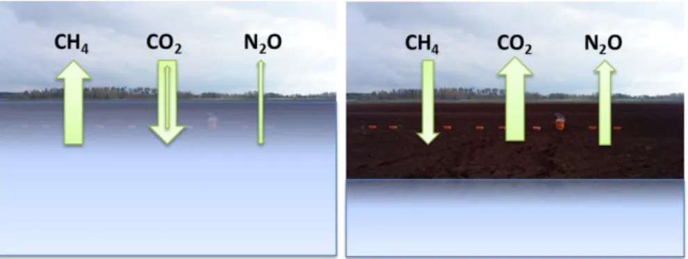
Between 28 and 64 % of peat subsidence has been estimated to originate from peat oxidation (Leifeld et al., 2011), which leads to the release of greenhouse gases such as carbon dioxide and nitrous oxide. A pristine peatland acts as a sink of carbon dioxide when vegetation grows and accumulates as peat. After drainage, the peatland turns into a source of carbon dioxide through microbial degradation of the organic material, whereby nitrogen is mineralised and made available through nitrification and denitrification (Figure 1). In nitrification, ammonia is oxidised to nitrite and then from nitrite to nitrate. If there is a lack of oxygen in the soil, for example due to high moisture, the nitrification process is inhibited, leading to production of nitrous oxide. Denitrification is an anaerobic process where microorganisms use nitrate instead of oxygen as an electron acceptor when degrading organic matter for energy. This process occurs (to a small extent) also in pristine peatland.

The third gas included in the greenhouse gas balance of peatlands is methane. Methane is formed in anaerobic conditions where molecules other than oxygen have to be used as electron acceptors in microbial degradation of organic material.

Figure 1. Schematic diagram of the nitrous oxide (N2O) producing processes of nitrification and

(17)

Figure 2. Schematic diagram of the fluxes of methane (CH4), carbon dioxide (CO2) and nitrous

oxide (N2O) to the atmosphere from (left) pristine peatland and (right) cultivated drained

peatland.

In contrast to the other two greenhouse gases (CO2 and N2O), there are

greater methane emissions from pristine peatlands than from drained peat (Figure 2). In drained peatlands, methane can be produced in deeper soil layers (below groundwater level) and may be partly consumed in aerated upper soil layers before it reaches the atmosphere.

It is important to consider the three greenhouse gases (CO2, N2O, CH4)

separately, since their production is the result of three different processes affected by various factors. The most important factors controlling emissions of all three gases are water content (aeration) and temperature. However, these factors impact upon production of the three gases in different ways. For example, methane production demands anoxic conditions (water saturation) while this limits carbon dioxide production, and nitrous oxide can be produced by denitrification in water-saturated conditions. When greenhouse gas emissions from drained cultivated organic soils are converted into CO2

-equivalents, it has been estimated that carbon dioxide contributes 85-95% of global warming potential (GWP), nitrous oxide contributes 5-15% and methane less than 1% (Grönlund et al., 2006; Maljanen et al., 2004). Therefore carbon dioxide appears to be the most important gas to investigate when considering mitigation options on drained organic soils.

3.3 Factors influencing greenhouse gas emissions from

peatland and carbon-rich soils

3.3.1 Cropping system

Around 7% of the agricultural area in Sweden is on organic soil, including gyttja and marl. Of this, around 50% is arable land, 40% pasture and unmanaged arable land and the rest is wetland or other land use types

(18)

(Pahkakangas et al., 2016). A subsidy system for the management of organic soils has been discussed in Sweden and many other countries. One of the issues discussed is the influence of different cropping systems on greenhouse gas emissions from organic soil.

In Sweden, a rule of thumb based on long-term measurements of subsidence of organic soils states that different cropping systems give different subsidence rates, e.g. permanent grassland gives a lower rate than row crops (Berglund, 1989). Since part of the subsidence originates from degradation of organic material, i.e. carbon dioxide emissions, row crops are considered to emit more carbon dioxide than grassland (Kasimir-Klemedtsson et al., 1997). However, one problem with using subsidence as an estimate of organic matter decomposition is how to distinguish between the different processes causing the subsidence (Glenn et al., 1993). The subsidence rate can be somewhere between 0.5 and 3 cm year-1 (Klöve et al., 2010; Grönlund et al., 2008; Berglund, 1996). The higher end of that range applies to open cropping systems (e.g. row crops) and the lower end to closed systems (e.g. permanent grassland). If these differences in subsidence rates are due to differences in oxidation rates between cropping systems, this should be reflected in huge differences in carbon dioxide emissions rates between cropping systems.

Others have studied this, with varying results. Several studies have compared emissions from soils under grassland and barley (Hordeum vulgare). In some of these, barley emitted less carbon dioxide than grassland (Maljanen et al., 2004; Lohila et al., 2003; Maljanen et al., 2001), while the opposite has been found in other studies (Lohila et al., 2004; Martikainen et al., 2002). Very few studies have included soils with row crops, but some have shown potato to emit less carbon dioxide than barley and grassland (Elsgaard et al., 2012; Lohila et al., 2004; Martikainen et al., 2002). In comparison with barley, nitrous oxide emissions have been found to be higher in grassland in some cases (Maljanen et al., 2003) and lower in others (Kasimir-Klemedtsson et al., 2009; Maljanen et al., 2004; Regina et al., 2004). Furthermore, whether the grassland is grazed or not can complicate the issue (Renou-Wilson et al., 2016). This variation in results shows the need for more research concerning the influence of cropping systems, especially row crops, on greenhouse gas emissions, since these are indicated to be the worst option. An adequate way to investigate this is to compare cropping systems adjacent to each other, where environmental factors, drainage intensity, soil type etc. are similar. Furthermore, a large number of replicate measurements, both temporally and spatially, are required.

This thesis investigated whether emissions of greenhouse gases differ between cropping systems in the same way as subsidence (Papers I and II).

(19)

3.3.2 Soil type

From studies of greenhouse gas emissions from cultivated organic soils, it is clear that the levels of emissions are different at different locations, for example within farms, within countries or between countries. This raises the question of the influence of soil type on greenhouse gas emissions. This issue is very important in the national and international calculations of greenhouse gas emissions to the atmosphere. The Intergovernmental Panel on Climate Change (IPCC) uses default emission factors of 5.7 and 7.9 tonnes CO2-C ha

-1

yr-1 for grassland and cropland, respectively, on boreal drained peatlands (IPCC, 2014). This difference in emissions between grassland and cropland can be due to peat quality and degree of decomposition (Wilson et al., 2015), rather than vegetation type, since different crops are grown on different soil types. It is of great importance that the emission factors are as accurate as possible, since they are part of the calculation and modelling of global climate change.

So far, the literature does not present any consistent conclusions regarding the soil factors that are most important for greenhouse gas emissions. In a broad sense, the botanical origin of the peat (Moore & Dalva, 1997) and the nutrient status of the original peat (Aerts & Ludwig, 1997) are of high importance for carbon dioxide production. For example, herbaceous peat and eutrophic conditions give higher carbon dioxide emissions than moss peat and mesotrophic conditions. Some different soil factors have been shown to influence soil carbon dioxide emissions, including: dissolved organic carbon (Bowen et al., 2009), pH, nitrate (NO3) content and degree of peat

decomposition (Szafranek-Nakonieczna & Stepniewska, 2014; Scanlon & Moore, 2000).

This thesis examined the effects of soil properties on greenhouse gas fluxes from organic soils (Paper I-III).

3.3.3 Drainage - groundwater level

Drainage intensity seems to be the most important factor controlling the greenhouse gas emissions connected to soil management (Beyer et al., 2015). Therefore it is important to investigate whether it is possible to find an optimum groundwater level where the greenhouse gas emissions are low with maintained agricultural activity. An optimum drainage depth of 30 cm has been suggested (Regina et al., 2015; Renger et al., 2002), which can coincide with optimum biomass production in some organic soil types (Berglund & Berglund, 2011). Furthermore, the lifespan of a fen peat can be extended from 130 years to more than 500 years by raising the groundwater level from 70 cm to 30 cm below the surface, which would be of great importance for farmers

(20)

(Renger et al., 2002). However, keeping the groundwater level constant is difficult and the degradation of the peat can be enhanced by wetting-drying cycles due to variations in groundwater level (Kechavarzi et al., 2007). Since even minimal drainage promotes rapid oxidation of peat (Kechavarzi et al., 2010), complete rewetting of the soil would be required in order to avoid greenhouse gas emissions.

In this thesis, small undisturbed soil cores were used in a laboratory study to investigate how increasing soil water suction (drainage) influences carbon dioxide emissions and whether different peat soil types respond differently to drainage.

(21)

4 Material and Methods

The work in this thesis was divided into two different parts, here referred to as ‘crop studies’ and ‘laboratory studies’. These parts are closely related, but with different main research questions and different working methods. The crop studies employed field-based methods where the impact of different cropping systems on greenhouse gas emissions was investigated (Papers I and II). These extensive soil analyses raised and answered questions closely connected to the laboratory studies. In the latter, a number of different peat soil types were monitored in the laboratory regarding soil properties and drainage depth correlated to carbon dioxideemissions (Paper III). The same sites/soils were covered in both types of study, but with some extra sites included in the laboratory investigations.

4.1 Site description and location

The farms visited for measurements and sampling were selected for their wide range of peat soil types or soils with high carbon content, and for the current farmer’s own interest and goodwill. The farms were active, with different kinds of cultivation. For the crop studies, farms with carrot and potato production in particular were selected, since these crops were most strongly associated with the main research question. The sites also had to be to be spread around Sweden, but at a reasonable travel distance from Uppsala.

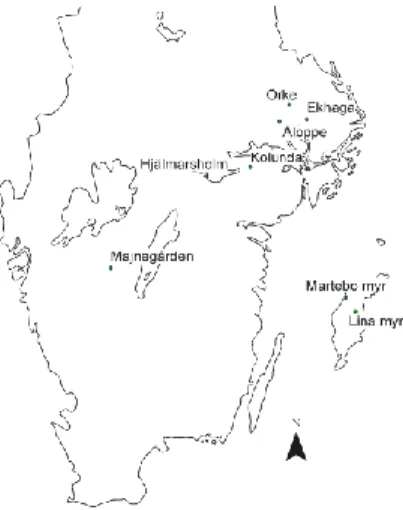
Figure 3. Map of southern Sweden showing the different peatland sites studied.

(22)

Six different sites in mainland Sweden and two on the island of Gotland were selected for the crop studies and soil sampling for the laboratory studies (Figure 3).

Kolunda is an active dairy farm with grassland and cereals grown for animal feed and is located south of Eskilstuna, on a drained mire area. The closest neighbouring site was a commercial business growing lawn grass. Lawn grass turf for sale needs a different management regime than ordinary grassland, for example cutting once a week, fertiliser and pesticides, rolling once a week to keep burrowing rodents under control etc. This treatment has led to greater compaction of the soil than on the adjacent grassland.

Hjälmarsholm is located close to Lake Hjälmaren and the area is part of the large drainage project Kvismaren-Hjälmaren. In 1870-1890, drainage channels were built to produce new agricultural land (Runefelt, 2008b). The area of Sweden’s fourth largest lake, Hjälmaren, was reduced and that of the nearby Lake Kvismaren was also reduced. Hjälmarsholm farm produces potatoes, carrots and cereals.

Lina myr on the island of Gotland was drained in the late 1940s after decades of discussions and conflicts. The area has limestone bedrock and consequently the peat soil is strongly influenced by high pH and visible particles originating from shells. The host farm, Norrbys, rears beef cattle and produces grassland and cereals for animal feed and sale, and sometimes also vegetables.

Martebo myr is located in the north-western part of the island of Gotland. The first drainage started in 1845, but it was not until the late 1800s that the approximately 1500-hectare mire and lake area was drained (Runefelt, 2008b). Today, large parts of Martebo myr consist of marl and peat-containing marl, with a subsoil of gyttja or lime-containing gyttja.

Åloppe is located outside Enköping but, unlike most of the other sites, it is not part of a large peatland area. The area where the measurements and sampling were performed is located at a small river in the lowest part of a field with a peat-forming environment. This area was then used for small-scale carrot cultivation and adjacent grass forage production. Åloppe is an organic farm with beef cattle and produces organic carrots.

Ekhaga is one of SLU’s research stations, focusing on organic cultivation. It is part of the SLU research farm Lövsta, outside Uppsala. The fields have not been fertilised for more than 10 years other than by green (crop biomass) manure and are otherwise managed by good crop rotation. The soil is gyttja clay.

Majnegården is located outside Falköping in south-west Sweden. Dairy cows have been kept on Majnegården for many years and crop production is

(23)

mainly for animal feed. The peat soil on the farm is influenced to varying degrees by the calcareous bedrock in the area. Due to great variation in soil type and soil properties, it was possible to use soil samples from three different locations within this same farm for the laboratory studies.

Örke is located 25 km north-west of Uppsala and is part of the peatland area Bälinge mossar. The drainage project at Bälinge mossar started in the beginning of the 20th century (McAfee, 1985). The experimental field at Örke has been abandoned for several years, but has previously been used for grass forage production for dairy cows.

A summary of all sites and the studies in which they were used is provided in Table 1, while peat properties and characteristics of the peat profile at all sites studied is presented in Table 2. Properties of topsoils and subsoils are shown in Table 3.

Table 1. The eight farms used in crop and laboratory studies and their respective code numbers in Papers I-III

Farm No. in Paper I No. in Paper II No. in Paper III

Kolunda 1 and 2 1 and 2 1

Hjälmarsholm 3 and 4 3 and 4 2

Lina myr 5 5 3

Martebo myr (peat) 6-7 6 5

Martebo myr (marl) 8-11 7-8 4

Åloppe 9

Ekhaga 10

Majnegården 6-8

Örke 9

Table 2. Soil profile description and peat depth for soils at the eight sites used in field and laboratory studies

Farm 0-20 cm layer 20-40 cm layer 40-60 cm layer Peat depth Kolunda Fen peat Peat with tree remains Peat mixed with gyttja 50-55 cm Hjälmarsholm Fen peat Peat with plant remains Gyttja clay 50-55 cm Lina myr Fen peat Marl/lime gyttja Clay gyttja 27 cm Martebo myr (peat) Fen peat Algae gyttja Lime gyttja 20-30 cm Martebo myr (marl) Peaty marl Lime gyttja (layered) Gyttja clay

Åloppe Fen peat Gyttja 20 cm

Ekhaga Gyttja clay Gyttja clay

Majnegården Fen peat Peat with plant remains Peat with plant remains 100 cm Örke Fen peat Fen peat Fen peat 150 cm

(24)

Table 3. Soil properties in the topsoil (upper table) and subsoil (20-40 cm; lower table) of the sites studied in Papers I-III

Farm pH (H2O) Loss on ign. % Total-C % Carbonate-C % Organic-C % Total-N % Bulk density g cm-3 Porosity vol-% Kolunda 11 5.6 53.5 27.2 0.0 27.2 1.6 0.54 71.6 Kolunda 21 5.7 83.0 39.6 0.1 39.5 2.0 0.37 77.3 Hjälmarsholm 11 5.4 78.3 39.2 0.1 39.1 2.6 0.34 79.9 Hjälmarsholm 21 6.0 86.1 41.6 0.5 41.1 2.1 0.312 80.02 Lina myr1 7.7 65.4 35.0 2.5 32.5 2.3 0.35 80.5 Martebo myr2 (peat) 7.5 64.9 35.8 2.9 32.9 2.3 0.39 76.7 Martebo myr2 (marl) 8.0 17.1 9.7 5.6 4.1 0.4 1.03 59.2 Åloppe1 5.7 40.5 18.3 0.1 18.2 1.4 Ekhaga1 6.6 11.5 1.1 57.0 Majnegården A2 6.1 72.8 37.1 0.3 36.8 3.2 0.38 77.6 Majnegården B2 7.5 48.4 26.3 5.3 21.0 2.0 0.45 77.4 Majnegården C2 5.0 79.9 37.3 0.2 37.1 3.0 0.29 80.9 Örke2 5.4 80.6 39.0 0.5 38.5 2.8 0.31 81.2 Farm pH (H2O) Loss on ign. % Total-C % Carbonate-C % Organic-C % Total-N % Bulk density g cm-3 Porosity vol-% Kolunda 11 4.2 78.2 27.5 0.0 27.5 2.2 0.29 82.7 Kolunda 21 5.0 77.2 27.0 0.0 27.0 1.9 0.25 85.8 Hjälmarsholm11 5.5 79.6 39.8 0.2 39.7 2.7 0.32 80.8 Hjälmarsholm21 4.9 92.2 46.5 0.1 46.4 2.1 Lina myr1 8.3 14.0 16.6 10.1 6.5 0.5 0.56 76.1 Martebo myr1 (peat) 6.3 76.4 36.3 0.1 36.1 2.7 0.32 80.7 Martebo myr1 (marl) 8.4 7.2 6.7 4.8 2.0 0.1 1.03 61.1 Åloppe1 6.2 17.8 8.0 0.0 8.0 0.5 Ekhaga1 5.2 6.4 1.0 62.0 Majnegården A2 6.1 82.5 43.5 1.0 42.6 2.9 0.19 87.8 Majnegården B2 7.6 59.0 27.4 4.4 22.9 1.5 0.23 88.6 Majnegården C2 5.2 87.0 42.2 0.3 41.8 2.7 0.17 88.5 Örke2 5.4 80.4 39.2 0.8 38.3 2.5 0.24 84.4 1

(25)

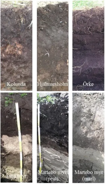
Figure 4. Images of the soil profile at Kolunda, Hjälmarsholm, Örke, Lina myr, Martebo myr (peat and marl). The three top pictures are of peat soils and the three lower pictures are of soil with a peat topsoil (left and centre images) or a marl topsoil and a marl subsoil (right image).

(26)

4.2 Crop studies

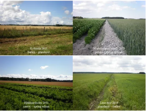
In the crop studies (Papers I and II), a comparison was made between two different crops grown in the same field or adjacent fields at each site. The soil type (parent material of the organic soil), peat depth, drainage intensity (same distance from drainage ditch) and weather conditions were similar for both crops, and only the crop and its associated management differed. Figure 5 shows some examples for four of the sites concerned. The crops grown were divided into three main groups, grassland, cereals and row crops, since subsidence data are often presented separately for these three groups. The grasslands were a mixture of grass, e.g. timothy (Phleum pratense), except for the lawn grass, which contained meadow grass (Poa pratensis) and red fescue (Festuca rubra). The cereals were: oats (Avena sativa), barley (Hordeum vulgare), spring oilseed rape (Brassica napus), spring wheat (Triticum aestivum) and spring triticale (Triticum aestivum/Secale cereale). The row crops were: carrot (Daucus carota), potato (Solanum tuberosum) and parsnip (Pastinaca sativa).

Figure 5. Examples of sites used in crop studies. Two different crops grown adjacent to each other.

(27)

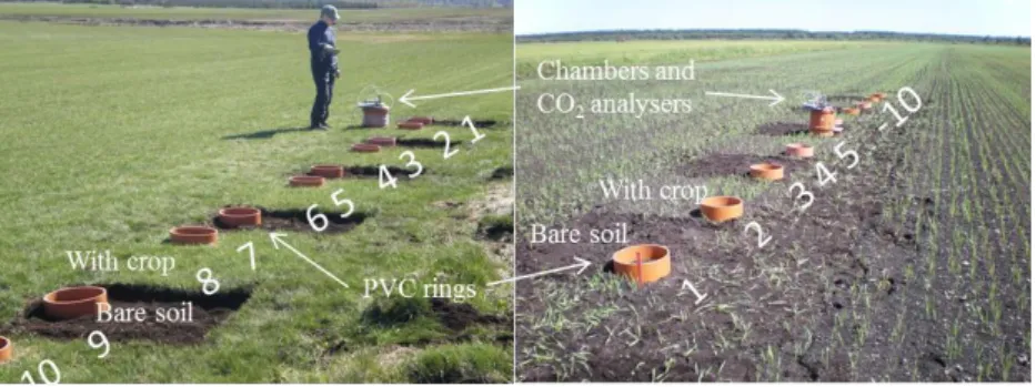
Ten study plots (approx. 1 m2) were laid out in a transect along the crop border, about 5 m into each crop at most sites (maximum 15 m) (see Figure 1 in Paper I). For the row crops, the study plots (2 m long) were placed along one row. The study plots were divided into five subplots with a crop and five with the crop manually removed (bare soil) in the beginning of the season and the surface kept bare thereafter by manual weeding once a month. Measurements of carbon dioxide emissions were made on plots with and without a crop. Sampling of nitrous oxide and methane was carried out on three of the plots with a crop (see Figure 2 in Paper II).

Within one hour prior to gas flux measurement, 0.25 m2 of plots with a crop (0.5 m row length for row crops) was cut to facilitate measurements. This area was then used for the gas flux measurements. On each measuring occasion, a new square/area of the study plot was used. The measuring area was also rotated in plots with bare soil, in order to achieve the same soil disturbance in both plot types. The set-up was the same at all study sites, see example in Figure 6. The study plots were managed by the respective farmer, in the same way as the rest of the field.

Gas measurements were performed once a month during the growing season (May-September). All measurements were made during daytime with the closed dark chamber method. Polyvinyl chloride (PVC) collars with a base area of 0.07 m2 were inserted 3 cm into the soil before measurement and PVC chambers were placed over the collars during incubation and sealed with a rubber seal. Two chambers were used for carbon dioxide measurements, one in each of the crops compared. The carbon dioxide measurements were performed at the same time in both crops, one collar at a time, following the transect of plots (starting at plot 1 and ending at plot 10), including bare soil plots.

Figure 6. Examples of the field set-up. Left: lawn grass at Kolunda. Right: newly sown barley at Lina myr.

(28)

Six chambers were used for measurement of the other greenhouse gases studied (N2O, CH4), three in each of the crops compared. Gas sampling was

performed on both crops from all six collars at the same time. The air in the closed chamber was sampled by circulating the air for 30 seconds between the chamber and a 22-mL vial sealed with a butyl rubber septum. During these 30 seconds, the air in the vial was exchanged seven times and a representative air sample was thus collected. Chamber air was sampled every 10 minutes for 40 minutes. The gas samples were analysed using gas chromatography (Perkin Elmer Clarus 500, USA).

Emission rates were calculated from the linear change in gas concentration in the chamber headspace (example in Figure 7). Measurements with good quality (i.e. linearity R2>0.85 for CO2 and N2O, R

2

>0.6 for CH4) were used for

flux estimations. Carbon dioxide, nitrous oxide and methane fluxes were estimated using equation 1:

F = (∆c/∆t * V/A * P*M)/(R*T) (Eq. 1)

where F is the gas flux in mg m-2 h-1 or µg m-2 h-1, ∆c/∆t is the average change in gas concentration during the closure time (ppm or ppb time-1), V is the volume of the chamber (m3), A is the base area of the chamber (m2), P is the atmospheric pressure (101 325 Pa), M the molecular mass of the gas (g mol-1), R is the gas constant (8.3145 J mol-1 K-1) and T is the sample temperature (K). In parallel with gas measurements, soil temperature and soil water content were determined. Soil temperature was measured with a thermometer at approximately 10 cm depth next to the collars to avoid disturbance. Volumetric soil moisture content in the upper 6 cm was determined with a WET sensor (Delta-T Devices Ltd, Cambridge, UK) in each collar immediately after gas sampling. An average of four measurements was used.

Figure 7. Examples of the linear increase in concentration of (left) nitrous oxide (N2O) and

(right) carbon dioxide (CO2) in the chamber headspace during closure time. R² = 0,9981 0 400 800 1200 1600 2000 0 10 20 30 40 50 N2 O (pp b ) Time (min) R² = 0,9971 300 350 400 450 500 550 0 1 2 3 4 5 6 CO 2 (pp m ) Time (min)

(29)

4.3 Field test of dark chambers

In a preliminary study, four issues related to the use of dark chambers for flux measurements were investigated:

i) The soil disturbance from inserting the PVC rings into the soil was tested by inserting one ring and leaving one ring just standing on the surface. The conclusion was that the effect of disturbance on gas measurements was negligible.

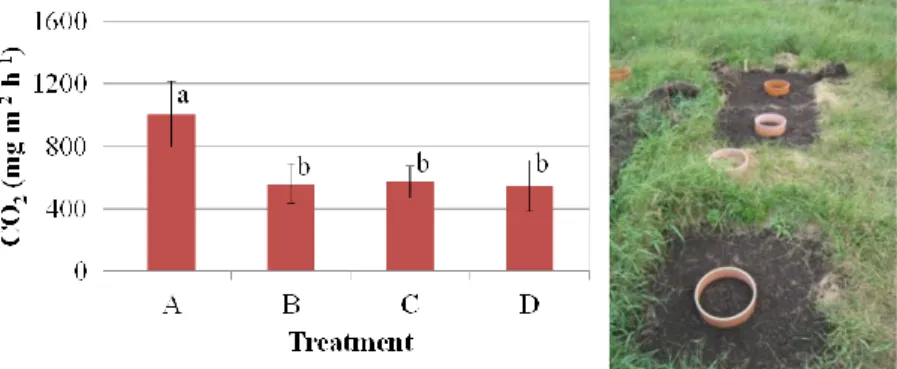
ii) Ways of keeping the bare soil plots free from vegetation were tested with four different approaches: cutting the vegetation to stubble just before measurement (A, control), removing the vegetation with a shovel just before measurement (B) or on the day before (C), or treating the surface with glyphosate before vegetation removal (D). As Figure 8 shows, the way in which the vegetation was removed did not matter for the carbon dioxide emissions.

iii) The impact of size of the dark chamber on calculated carbon dioxide emissions, because the size of the chamber changed from year 1 to year 2 in the crop studies. The results showed that different chamber sizes did not influence the carbon dioxide emissions.

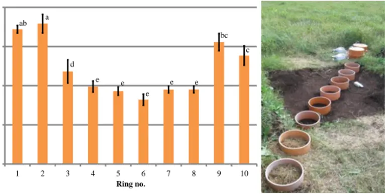
iv) Possible border effects in bare soil plots were studied by measuring carbon dioxide in a line diagonal through a 2 m2 plot with the vegetation removed several days before measurement (Figure 9). The results showed a border effect.

Figure 8. Effects of four different methods of vegetation removal before measurement on carbon dioxide (CO2) flux from field plots. A) Vegetation cut at ground level, B) vegetation removed by

shovel just before measurement, C) vegetation removed by shovel on the day before measurement and D) vegetation removed by shovel after treatment with glyphosate. Bars indicate mean values of four measurements with four replicates (n=16) and error bars indicate standard deviation. Different letters denote significant differences between treatments. (Photo: Isak Öhrlund)

(30)

Figure 9. Border effects on carbon dioxide (CO2) emissions from bare soil plots. Ring nos. 1-2

and 9-10 were on vegetated soil (grass cut) outside the bare soil plot. Bars indicate mean values of six replicates (n=6) and error bars indicate standard deviation. Different letters denote significant difference between rings. (Photo: Isak Öhrlund)

4.4 Laboratory studies

In the laboratory studies (Paper III), comparisons were made between 13 different soils regarding their carbon dioxide emissions in relation to soil type and drainage. Topsoil samples were collected in autumn 2011 at nine different agricultural sites in southern Sweden. At two of the sites (Majnegården (three soils) and Örke), subsoil samples were also collected from the same spots, giving a total of 13 different soils.

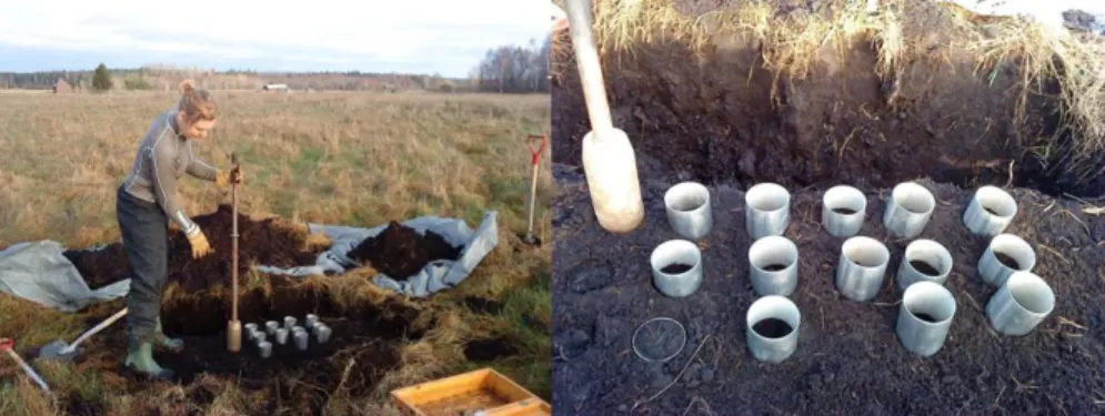
Prior to soil sampling, surface vegetation was removed and undisturbed soil cores were sampled in steel cylinders (Ø7.2 cm, 10 cm high) at approx. 5-15 cm depth for topsoil samples and at 20-50 cm depth for subsoil samples (Figure 10). Replicates were taken from each soil to be used in carbon dioxide emission measurements and soil analyses. Upon extraction, the cylinders were sealed at both ends with plastic lids and stored in wooden boxes. The boxes were transported directly from the field to a cold store (5 °C), where they were kept until the experiment started.

At the start of the experiment, soil samples were distributed into seven different boxes, which were assumed to be independent blocks in the statistical analysis. Each box contained one sample from each of the 13 soils. All boxes were treated separately, but in the same way as the other boxes. The boxes were kept in storage at 5 °C and brought into the experiment one at a time. Before the start of measurements, the relevant box was kept at room temperature (20 °C) for two days and then the 13 soil cylinders were soaked in water for three days until water-saturated.

ab a d e _e e e e bc c 0 400 800 1200 1600 1 2 3 4 5 6 7 8 9 10 CO 2 (mg m -2 h -1) Ring no.

(31)

Figure 10. Sampling of undisturbed soil cores at Örke.

During these first days the samples were carefully observed and replaced if necessary due to e.g. earthworm disturbance in the samples. The 13 samples were then placed on a suction sand bed (Figure 11) for successive adjustment to a soil water suction head of 0.5 and 1.0 m water column (approx. 5 and 10 kPa). In addition, three of the boxes of soil samples were adjusted to a suction head of 0.75 m water column, and one of these boxes was subjected to an additional two suction steps, 0.25 and 1.5 m water column. At each suction step, it took about seven days to reach equilibrium, i.e. when no more drainage of water was observed.

Prior to carbon dioxide emissions measurements, the soil samples were weighed for water content calculations. When all carbon dioxide emissions measurements were finished, the soil cores in three of the boxes were divided into two new samples, one for the freezer (-18 °C) and one for the fridge (+5 °C). These new soil samples were then used for different soil analyses. Soil cores from the four remaining boxes were dried for 72 h at 105 °C and weighed for dry weight-based emissions calculations. The mean dry weight of soil samples in these boxes was used for the corresponding soil samples in the other boxes.

For the carbon dioxide emission measurements, polypropylene jars with a volume of 1140 cm3 (Ø 11 cm, 12 cm high) were used (Figure 12). This size of jar was chosen to fit the size of the soil sample cylinders. The jars were closed with air-tight screw lids equipped with two injection needles (Ø 0.8 mm, 40 mm long). The needles were inserted through the lid and glue was used around the insertion points to ensure the jars were air-tight.

(32)

Figure 11. Picture and simplified description of a sand bed used to apply suction to soil samples. The difference in height between the suction regulator and the middle of the soil samples determines the amount of suction. Suction heads between 0 and 1.0 m can be applied. Examples of suction heads used in the laboratory studies on the right side of the picture.

The carbon dioxide emissions fluxes from the different soils were determined by placing a soil sample cylinder in a jar (without the plastic lid at the top of the cylinder), directly closing the screw lid and then connecting the injection needles in the lid via plastic tubing to a portable infrared CO2 analyser

(Carbocap CO2 Probe GMP343, Vaisala Ltd, Vantaa, Finland) for 5-10

minutes, with a measurement every 30 seconds (Figure 12). A longer closure time in the jar was used at lower emissions rates.

Gas measurements were made on one sample at a time until all samples (1-13) were measured. The measuring procedure was performed twice at each measuring occasion (suction step). The jar and the gas analyser were allowed to ventilate between each sample. The carbon dioxide emissions from the soil were calculated by the linear increase in carbon dioxide concentration in the jar during the closure time.

In general, emissions fluxes with linearity higher than r2=0.85 were used, but measurements with lower r2 were included if they did not exhibit any obvious error on visual inspection. Negative values were omitted. Most of the omitted values were obtained during near water-saturated measurements. Mean values of the two measurements per occasion were used in the statistical analysis, but in cases where values were omitted only one value was used.

(33)

Figure 12. Left: Infraredcarbon dioxide (CO2) analysers connected to the closed measuring jars

with soil cores inside. Right: Measuring jars and soil core steel cylinders (foreground) and boxes with samples (rear).

The carbon dioxide emission fluxes were calculated using Eq. 2 (described in Kainiemi et al. (2015)) and then divided by the dry soil weight:

F=(∆c/∆t*V*P*M)/(R*T) (Eq. 2)

where F is the carbon dioxide flux in mg CO2 min

-1

, ∆c/∆t is the average change in carbon dioxide concentration during closure time (ppm min-1), P is the atmospheric pressure (101 325 Pa), V is the volume air in the jar (L), M is the molecular mass of CO2 (g mol

-1

), R is the gas constant (8.3145 J mol-1 K-1) and T is the temperature (K). Air volume (V) was calculated by subtracting the volume of the cylinder from the total volume of the jar. The temperature was constant at 20 °C, the indoor temperature in the laboratory.

4.5 Soil analysis

To characterise the soil types in both the crop and laboratory studies, physical and chemical soil analyses were carried out (Paper I-III). In the crop studies, soil sampling and soil profile description were performed at one representative spot within the study site. Analyses of field plot soils were carried out in the laboratory and involved determination of humification degree, pH, loss on ignition, nitrogen and carbon content, dry bulk density, water content at different soil water suction heads, porosity, air-filled pore space. In the laboratory studies, extensive soil analyses were carried out on the 13 different soils studied. In addition to the analyses listed for field plot soils, mineral nitrogen content and water-extractable organic carbon were determined.

The humification degree (H1-H10) of the peat soils was determined according to von Post (1922). Soil pH was measured at a soil-solution ratio of

(34)

1:2 in crop studies and 1:5 in laboratory studies, with deionised water. Organic matter content (loss on ignition) was measured by dry combustion at 550 °C for 24 h after pre-drying at 105 °C for 24 h. Total nitrogen (tot-N), total carbon (tot-C) and carbonate-C content were determined by dry combustion on a LECO CN-2000 analyser (St. Joseph, MI, USA).

M

ineral N (nitrate (NO3) and

ammonium (NH4)) were determined on a TRAACS 800 AutoAnalyzer

(Bran+Luebbe, Germany).

Water-extractable organic carbon, WEOC, here presented as total and filtered WEOC (WEOCtot and WEOCfil, respectively) was determined by a

modified version of the method of Ghani et al. (2003). Soil samples were placed in 50 mL polypropylene centrifuge tubes and deionised water was added to the soil samples in a soil-water solution of 1:5. The soil-water samples were centrifuged for 20 min at 3500 rpm after 1 h on an end-over-end shaker and the supernatant was decanted into new tubes and analysed for WEOCtot on a Shimadzu TOC-5000A. The supernatant was then filtered

through a 0.45 µm membrane filter and analysed again for WEOCfil. In

parallel, a similar amount of soil as in the centrifuge tubes was used for dry weight determination at 105 °C for 24 hours. The analytical data were then recalculated using the dry weight data and the results were presented as mg WEOCtot or WEOCfil per g total carbon in the soil.

Undisturbed soil cores (Ø7.2 cm, 10 cm high) were used for analysis of soil physical properties. Dry bulk density and volumetric water content at a suction head of 0.05, 0.3, 0.5, 0.7, 1.0 and 6.0 m water column (approx. 0.5, 3, 5, 7, 10 and 60 kPa) were determined. Porosity was calculated from particle density and dry bulk density, while air-filled pore space at different suction heads was calculated from water retention data.

4.6 Statistical analysis

In the crop studies, the carbon dioxide emissions data did not meet normality and homoscedasticity requirements, and therefore they were ln-transformed before the two-way ANOVA and two-sample t-tests. The nitrous oxide and methane emissions data did not follow normal distribution and therefore non-parametric statistics was used (Mann-Whitney test and Kruskal-Wallis test).

In the laboratory studies, pair-wise comparisons of the carbon dioxide emissions data were made with two-sample t-test and Tukey’s adjustment. Two-way ANOVA with the general linear model (GLM) procedure was used to test for differences in CO2 emissions caused by suction head increments and

soils, with box used as block effect. For the ANOVA, the data were square-root transformed to meet the requirements of normality and equal variances.

(35)

Correlations between CO2 emissions and soil factors were tested with

non-linear and non-linear regression.

In the remainder of this thesis mean values are presented, together with standard deviation and median values with first and third quartiles. All statistical analyses were carried out in Minitab 17 (Minitab Inc. USA).

(36)

(37)

5 Results and Discussion

5.1 Cropping system (Papers I-II)

As shown in Papers I and II, the carbon dioxide, nitrous oxide and methane fluxes from the soil under different crops varied depending on the scale at which the data were evaluated. The gas emissions data were evaluated on three different scales:

At the first scale, a two-way ANOVA was used to evaluate the difference in carbon dioxide emissions between the three main groups of crops (grassland, cereals, row crops). For this, all data from all sites were used. It was found that in terms of total carbon dioxide emissions (plots with crop), grassland was a greater emitter of carbon dioxide than cereals and row crops (Table 4). In terms of carbon dioxide emissions from bare soil, grassland emitted more than row crops but not cereals. For nitrous oxide emissions, the Kruskal-Wallis test did not show any differences between the three groups of crops (Table 4).

At the second scale, most of the seasonal average carbon dioxide emissions from individual sites showed no difference between the crops compared, but with some exceptions (see Paper I).

Table 4. Total carbon dioxide (CO2) emissions (with crop), bare soil CO2 emissions and nitrous

oxide (N2O) emissions from the three groups of crops. The CO2 emissions are means with

standard deviation in brackets and N2O emissions are median values with first and third quartile

in brackets. Note: Different letters denote significant difference between the three groups of crops Total CO2 (mg m-2 h-1) Bare soil CO2 (mg m-2 h-1 ) N2O (µg m-2 h-1) Grassland1 1170b (573) 749b (524) 72a (6, 389) Cereals2 808a (447) 633ab (362) 72a (8, 498) Row crops3 803a (404) 624a (312) 30a (6, 406) 1 n=75 (N2O) and 170 (CO2), 2 n=93 (N2O) and 200 (CO2), 3 n=66 (N2O) and 137 (CO2).

(38)

The seasonal average total carbon dioxide emissions from sites measured in 2010 revealed that only one paired comparison of crops at a site was significantly different (Figure 13). This was the Hjälmarsholm site, where carrots emitted more carbon dioxide than spring oilseed rape. The corresponding graphs for nitrous oxide andmethane (Figures 14 and 15) did not show any significant difference between the crops compared, as also shown in Paper II.

Figure 13. Seasonal average of total soil carbon dioxide (CO2) emissions (plots with crop; bars

show standard deviation) from crop pairs at the sites, 2010. Kolunda, Hjälmarsholm, Lina myr and Martebo myr 1 are peat soils and Martebo myr 2 and 3 are peaty marls. Bars marked with * are significantly higher (p>0.05) than those for the comparison crop.

Figure 14. Seasonal average of nitrous oxide (N2O) emissions (median, first quartile (lower error

bars) and third quartile (upper error bars)) from crop pairs at the sites, 2010. Kolunda, Hjälmarsholm, Lina myr, Martebo myr 1 and Åloppe are peat soils, Martebo myr 2 and 3 are peaty marls and Ekhaga is gyttja clay.

0 500 1000 1500 2000 2500

Kolunda 1 Kolunda 2 Hjälmarsholm Lina myr Martebo myr 1 Martebo myr 2 Martebo myr 3

CO 2 (m g m -2 h -1) * 0 1000 2000 3000

Kolunda 1 Kolunda 2 Hjälmarsholm Lina myr Martebo myr 1 Martebo myr 2 Martebo myr 3 Åloppe Ekhaga

N2 O (µ g m -2 h -1)

(39)

Figure 15. Seasonal average of methane (CH4) emissions (median, first quartile (lower error bars)

and third quartile (upper error bars)) from crop pairs at the sites, 2010. Kolunda 1-2, Hjälmarsholm, Lina myr, Martebo myr 1 and Åloppe are peat soils, Martebo myr 2 and 3 are peaty marls and Ekhaga is gyttja clay.

At the third scale, cropping systems on individual carbon dioxide measuring occasions were compared. The results showed several significant differences between crop pairs compared within individual sites, but the trend sometimes changed over the season and between sites (Figure 2 in Paper I). Nitrous oxide emissions did not show any significant difference between the pairs of crops compared on any measuring occasion (Figure 3 in Paper II). Methane fluxes were not evaluated at this scale, due to low fluxes.

The overall finding from evaluation of the data in Papers I and II was that there were differences between cropping systems regarding greenhouse gas emissions, but the results were not conclusive.

One reason for the significantly higher total carbon dioxide emissions from grassland (Table 4) was the longer vegetation period, i.e. root-induced respiration during a longer time, than for cereals and row crops. This does not necessarily mean more degradation of the soil material from grasslands, but rather a larger proportion of root respiration. In an ecosystem exchange approach, grassland would also take up carbon dioxide during a longer period than cereals and row crops, thus compensating for the soil emissions. Lohila et al. (2004) have reported that both barley and grass have larger uptake of carbon dioxide than respiration during their most intense growing period, barley during six weeks and grass for a longer time. Due to this, grass can sequester more carbon dioxide from the atmosphere than barley (Martikainen et al., 2002). It is important to bear in mind that different crops have varying rates of CO2 uptake. Furthermore, microbial activity increases when

-20 -15 -10 -5 0 5

Kolunda 1 Kolunda 2 Hjälmarsholm Lina myr Martebo myr 1 Martebo myr 2 Martebo myr 3 Åloppe Ekhaga

CH 4 (µ g m -2 h -1)

(40)

rhizodeposition increases (Kuzyakov, 2002) and different crops can affect this in different ways.

The focus in the crop studies (Paper I) was on the degradation of the peat soil, subsidence and emissions of greenhouse gases from the soil and how vegetation affected these parameters. It was not on the ecosystem and the fluxes of gases within this large system, studies of which would have required a different type of measurement equipment and different analytical strategies. With opaque (dark) chambers, photosynthesis is negligible so the fluxes measured originate only from degradation of the soil, root respiration and root-induced soil degradation. According to Kuzyakov and Gavrichkova (2010), the total carbon dioxide emissions from soil have five main sources: root respiration, rhizomicrobial respiration, microbial respiration, basal respiration and a priming effect (Figure 16).These five main sources can be divided into two main groups: plant-derived carbon dioxide and soil organic matter-derived carbon dioxide.

The crop was cut before measurement, which further decreased the impact of photosynthesis. In an attempt to differentiate between the different fluxes, carbon dioxide was measured in plots with a crop and in plots with the crop removed in the beginning of the season and then kept clear of vegetation (Figure 17). The plots were adjacent to each other and thus differed only in presence/absence of the crop. This approach provided an indication of the plant-derived respiration, i.e. the part of the total soil carbon dioxide that comes from root respiration and root-induced soil respiration.

Figure 16.Sources of total carbon dioxide (CO2) emissions from soil, modified from Kuzyakov

and Gavrichkova (2010). These five main sources are divided into two groups: (left) plant-derived CO2 and (right) soil organic matter-derived CO2.

(41)

Figure 17. Different fractions of carbon dioxide (CO2) captured in the dark chambers during

measurement from soil (left) without a crop and (right) with a grass crop.

However, the carbon dioxide emissions from plots without a crop can be influenced by the vegetation surrounding the plot (Figure 17), i.e. root-derived respiration can escape into bare soil plots. Another drawback with the bare soil approach is the possibility of easily degradable material, such as roots and other plant material, still remaining in the soil after the vegetation is removed (Shurpali et al., 2008). Both of these issues lead to higher carbon dioxide emissions than from soil degradation alone.

Another observation regarding the differences between crops is that row crops, e.g. potato and carrots, are usually grown in ridges, which dry out more on the top compared with ‘flat’ soil. It was found that the soil moisture content was usually lower at the top of the ridges compared with under cereals (Paper I). This could lead to lower carbon dioxide emissions from row crops due to lack of moisture for soil-degrading microbes, which was seen in the comparison with grassland, but not with cereals (Table 4). This could be the reason why potatoes have been reported to emit less carbon dioxide than cereals and grassland in Elsgaard et al. (2012).

Nitrous oxide was measured only in plots with a crop, so it was not possible to evaluate whether there were any differences in nitrous oxide emissions with or without vegetation (Paper II). In plots a with crop, the plants could be a competitor for soil nitrogen and could therefore lower nitrous oxide production compared with plots without a crop. All crops studied use soil nitrogen during their growing period, but the differences between annual and perennial crops

(42)

could be greater outside the measuring period due to tillage in annual crops and due to perennial crops competing for nitrogen early and late in the season.

Another difference between the crops was fertilisation. The crop studies found no relationship between nitrogen addition and nitrous oxide emissions, although the amount added varied from no fertilisation for decades to approximately 270 kg N ha-1 yr-1 (Paper II). Several other studies have examined the relationship between nitrogen fertilisation and nitrous oxide emissions from peat soils. Some have found a connection (Koops et al., 1997; Velthof & Oenema, 1995) and some not (Maljanen et al., 2004; Regina et al., 2004; Flessa et al., 1998). Lindén (2015) showed that the supply of plant-available soil nitrogen during the growing season averaged 166 kg N ha-1 (range: 78-274 kg), compared with 60-80 kg N ha-1 in mineral soil, which indicates that fertilisation might be of less importance for the nitrous oxide flux in these nitrogen-rich soils compared with mineral soils.

The lack of differences in nitrous oxide emissions between crops in the crop studies (Paper II) could have originated from high variation in measurements. Large variations in nitrous oxide emissions, both spatially and temporally, are commonly reported in other studies on different agricultural soils (Rees et al., 2013; Kasimir-Klemedtsson et al., 2009; Regina et al., 2004; Yamulki & Jarvis, 2002).

The measurements in the crop studies (Papers I and II) were only made during summer (May-September), which is important to remember in interpretation of the results. For example, the annual nitrous oxide emissions from the sites were most likely underestimated, since a significant proportion of nitrous oxide emissions from organic soils take place during winter (Maljanen et al., 2004). On the other hand, carbon dioxide emissions are more temperature-dependent and have their peak during summer. Emissions of methane are especially water dependent, so a warm, dry summer slows down methane production.

The question that arises is why subsidence is lowest in grassland cropping systems, when the carbon dioxide emissions may be highest from grassland (Table 4). Erosion probably plays a major part in this. Peat particles are very small and of low weight, and thus easily blown away. On windy days, it is possible to see clouds of wind-blown peat above bare (unvegetated) peat. Since the soil in row crop cultivation stays bare for a large proportion of the year, it is exposed to erosion for a longer time than grassland. Furthermore, the eroded peat material from an open field may blow over to adjacent grassland, where it becomes trapped in the grass, as discussed by Parent et al. (1982) and Irwin (1977), thus building up the peat layer there. Another reason for the varying subsidence rate can be a selection bias, in that different peat soil types are used

(43)

for different crops. Row crops are grown on the best soils, i.e. nutrient-rich and with good drainage, while permanent grassland grows on less fertile soils with poorer drainage. Apart from being suitable for intense cultivation, nutrient-rich soil is probably also a good habitat for microorganisms that degrade the peat.

The results presented in this thesis would have been completely different if, for instance, only the Hjälmarsholm site had been used for measurements. If that had been the case, carrots would have been found to be the greatest emitter of greenhouse gases. It is also important to carry out measurements several times during the growing season, since the differences in greenhouse gas emissions between crops could change over the season. Ideally, measurements should be made continuously during the whole year. The greatest strength in the crop studies reported in this thesis was that measurements were made on a number of occasions at several different sites with varying soil types and cropping systems.

The overall conclusion from the crop-studies is that no specific crop can be considered as a way to mitigate climate change by reducing greenhouse gas emissions from drained cultivated peat and carbon-rich soils during the growing season.

5.2 Soil type (Papers I-III)

In the crop studies, it was observed that site-specific effects were a key factor for the greenhouse gas emissions rather than the cropping system (Papers I and II). This led to the laboratory studies, where it was possible to investigate the relationship between soil properties and carbon dioxide emissions under controlled conditions (Paper III). As can be seen from Table 3, there were large variations in soil properties for the peat soils and even larger variations when peaty marl and gyttja clay were included in the comparison.

The results from both the crop and laboratory studies did not demonstrate a clear and simple relationship between any soil property and carbon dioxide emissions (see examples in Figure 18 and Papers I and III). There were no statistical correlations between field carbon dioxide emissions and any of the measured soil properties. As Figure 18 shows, there was a linear correlation between laboratory carbon dioxide emissions and total carbon, loss on ignition, dry bulk density, total nitrogen and porosity when Martebo myr (marl) was included, while when this soil was excluded, as in Paper III, there was no correlation. Peaty marl differs from the other (peat) soils and its inclusion in this type of analysis may not be justified. On the other hand, in the correlations of field carbon dioxide emissions in Figure 18, both Martebo myr (marl) and

(44)

Ekhaga (gyttja clay) were included. However, Figure 18 shows that field and laboratory measurements correlated with each other.

Figure 18. Correlations between field and laboratory carbon dioxide (CO2) emissions and selected

soil factors: a) total carbon (tot-C), b) loss on ignition, c) dry bulk density, d) pH, e) total nitrogen (tot-N) and porosity. Field measurements (squares, secondary y-axis) are mean CO2 emissions for

the season 2010 (bare soil plots), while laboratory measurements (triangles, primary y-axis) are from a soil water suction head of 1.0 m water column. Marl and gyttja clay are marked in the graphs and all other soils are peat.

Marl Marl 0 400 800 1200 0 100 200 300 0 10 20 30 40 50 CO 2 (mg m -2 h -1) CO 2 (mg g -1 dry so il min -1) tot-C (%) a) Marl Marl Gyttja clay 0 400 800 1200 0 100 200 300 0 20 40 60 80 100 CO 2 (mg m -2 h -1) CO 2 (mg g -1 dry so il min -1) loss on ignition (%) b) Marl Marl Gyttja clay 0 400 800 1200 0 100 200 300 0 0.2 0.4 0.6 0.8 1 1.2 CO 2 (mg m -2 h -1) CO 2 (mg g -1 dry so il min -1)

dry bulk density (g cm-3)

c) Marl Marl Gyttja clay 0 400 800 1200 0 100 200 300 5 6 7 8 9 CO 2 (mg m -2 h -1) CO 2 (mg g -1 dry so il min -1) pH d) d) Marl Marl 0 400 800 1200 0 100 200 300 0 1 2 3 4 CO 2 (mg m -2 h -1) CO 2 (mg g -1 dry so il min -1) tot-N (%) e) Marl Marl Gyttja clay 0 400 800 1200 0 100 200 300 50 60 70 80 90 CO 2 (mg m -2 h -1) CO 2 (mg g -1 dry so il min -1) porosity (%) f)

(45)

Figure 19 provides a good indication of how carbon dioxide emissions can vary between soils and within soils (error bars). In the laboratory studies, Martebo myr (peat) had the highest carbon dioxide emissions and Martebo myr (marl) had the lowest (see also Paper III). These two soils were located in the same peatland area, just a few kilometres apart. Martebo myr (peat) is highly influenced by its calcium carbonate (CaCO3) rich marl subsoil. The

Majnegården A-C soils were also taken from the same farm, illustrating how peat soil properties and carbon dioxide emissions can differ within a relatively small area (Table 3, Figure 19 and Paper III).

Figure 19. (Upper diagram) Emissions of carbon dioxide (CO2) from the nine topsoils studied, at

a soil water suction head of 1.0 m water column in laboratory studies and (lower diagram) mean seasonal CO2 emissions (bare soil plots) in 2010 in crop studies. Notes: Different letters denote

significant difference between soils (Tukey´s adjustment). Åloppe and Ekhaga data are from Wall (2011). 0 400 800 1200 1600 CO 2 (m g m -2 h -1) a ab a a ab ab ab b 0 100 200 300 400 CO 2 (m g g -1 d ry soi l m in -1) c bc ab a a a ab ab d