Does tax simplification yield more equity and efficiency? An empirical analysis for Germany

econ

stor

www.econstor.eu

Nutzungsbedingungen:

Die ZBW räumt Ihnen als Nutzerin/Nutzer das unentgeltliche, räumlich unbeschränkte und zeitlich auf die Dauer des Schutzrechts beschränkte einfache Recht ein, das ausgewählte Werk im Rahmen der unter

→ http://www.econstor.eu/dspace/Nutzungsbedingungen nachzulesenden vollständigen Nutzungsbedingungen zu vervielfältigen, mit denen die Nutzerin/der Nutzer sich durch die erste Nutzung einverstanden erklärt.

Terms of use:

The ZBW grants you, the user, the non-exclusive right to use the selected work free of charge, territorially unrestricted and within the time limit of the term of the property rights according to the terms specified at

→ http://www.econstor.eu/dspace/Nutzungsbedingungen By the first use of the selected work the user agrees and declares to comply with these terms of use.

zbw

Peichl, Andreas; Fuest, Clemens; Schaefer, Thilo

Working Paper

Does tax simplification yield more equity and

efficiency? An empirical analysis for Germany

Finanzwissenschaftliche Diskussionsbeiträge / Finanzwissenschaftliches Forschungsinstitut an der Universität zu Köln, No. 06-5

Provided in cooperation with:

Universität zu Köln

Suggested citation: Peichl, Andreas; Fuest, Clemens; Schaefer, Thilo (2006) : Does tax simplification yield more equity and efficiency? An empirical analysis for Germany,

Finanzwissenschaftliche Diskussionsbeiträge / Finanzwissenschaftliches Forschungsinstitut an der Universität zu Köln, No. 06-5, http://hdl.handle.net/10419/23255

Finanzwissenschaftliche Diskussionsbeiträge Nr. 06 - 5

Does Tax Simpli…cation yield

more Equity and E¢ ciency?

An empirical analysis for Germany

by

Clemens Fuest , Andreas Peichlz_{, Thilo Schaefer}x

July 2006

Center for Public Economics University of Cologne

ISSN 0945-490X ISBN-10 3-923342-59-4 ISBN-13 978-3-923342-59-4

Center for Public Economics, University of Cologne, Albertus-Magnus-Platz, 50923 Cologne, Germany. E-Mail: [email protected]

z_{Center for Public Economics, University of Cologne, Albertus-Magnus-Platz, 50923 Cologne, Germany.}

E-Mail: [email protected]

x_{Center for Public Economics, University of Cologne, Zuelpicher Str. 182, 50937 Cologne, E-Mail:}

Abstract

This paper investigates the impact of tax simpli…cation on various indicators of the e¢ ciency of the tax system and on the distribution of income. The analysis is based on a simulation model (FiFoSiM) using German income tax and household survey microdata. We model tax simpli…cation as the abolition of a set of deductions from the tax base included in the German income tax system. We …nd that this form of tax base simpli…cation leads to a reduction in the use of professional tax advice, a more equitable income distribution and an increase in tax revenue. If these measures are combined with a reduction of income tax rates to preserve revenue neutrality, the e¤ects depend on the type of rate schedule adjustment. The combination with a ‡at rate tax implies redistribution in favour of very high incomes, and an overall increase in income inequality. E¢ ciency e¤ects in terms of changes in marginal tax rates and labor supply e¤ects are mixed. The combination with a rate schedule adjustment which preserves the directly progressive rate schedule yields a tax reform which reduces the inequality of after tax incomes. We conclude that tax simpli…cation may improve the e¢ ciency of the tax system without increasing inequality of after tax income.

JEL Codes: D3, H2, J22

Keywords: Income distribution, polarisation, tax simpli…cation, ‡at tax

Acknowledgement: The authors would like to thank Christian Bergs, Axel Schmidt and the participants of the 8th Nordic Seminar on Microsimulation Models for their helpful contributions. The usual disclaimer applies.

Contents

List of Tables 3

List of Figures 3

1 Introduction 4

2 FiFoSiM: Database and Model 6

3 Tax simpli…cation scenarios 6

4 Complexity of the tax system 9

5 Distributional e¤ects 10

6 Tax simpli…cation and e¤ective marginal tax rates 13

7 Labour supply e¤ects 14

7.1 Model . . . 14 7.2 Results . . . 15

8 Summary and conclusion 16

Appendix 17

List of Tables

1 Tax rate parameters . . . 8

2 Regression on the use of tax consultants . . . 9

3 Probability of using a tax consultant . . . 10

4 Percentage change of household equivalence weighted net income . . . 11

5 Changes in e¤ective marginal tax rates in percentage points . . . 13

6 Full time equivalents . . . 16

7 Scenarios and …scal e¤ects in billione . . . 18

8 Deciles of weighted equivalent net incomes . . . 18

9 Percentage changes of net income in cat. A. . . 19

10 Percentage changes of net income in cat. B. . . 19

List of Figures

1

Introduction

The simpli…cation of the tax system is a key objective of many income tax reform proposals in various countries1. This is not only because complexity leads to high compliance costs for taxpayers and to tax evasion. The complexity of the income tax system is also widely seen as an obstacle to fairness and e¢ ciency beyond costs of administration and compliance. For instance, complexity is thought to be a barrier to achieving a fair distribution of the tax burden because it might allow taxpayers with high incomes to use tax loopholes and reduce their tax burden.

Given the importance attributed to tax simpli…cation in tax reform debates, there is sur-prisingly little empirical research on the impact of tax simpli…cation on the equity and the e¢ ciency of the tax system. To some extent, this may be due to the fact that the theoretical and empirical analysis of tax simpli…cation faces considerable conceptual problems. In partic-ular, tax simpli…cation itself is not a clearly de…ned concept. It is not always clear whether changes in the tax law increase or decrease the complexity of the tax system. In many cases, measures which broaden the tax base are considered to be simpli…cations. But in some cases (e.g. the taxation of the imputed rent of owner occupied housing) tax base broadening may also complicate the system.2 _{Despite these di¢ culties, it is important to investigate whether}

the idea that tax simpli…cation also leads to a more equitable and a more e¢ cient tax system can be supported empirically.

The present paper uses a simulation model based on German micro data to quantify the impact of tax simpli…cation on the use of professional tax advice, the distribution of after tax income, the marginal income tax rates faced by di¤erent types of taxpayers, and the supply of labour. The use of professional tax advice is an indicator of both the complexity of the tax system and the compliance cost. The change in marginal income tax rates is of interest because marginal tax rates may be considered as rough indicators for the distortions caused by the tax system. Our analysis is based on a simulation model for the German tax and transfer system (FiFoSiM)3 _{using income tax microdata and household survey data. The qualitative results}

should be of interest to a wider range of countries.

We model tax simpli…cation as the abolition of a set of deductions from the tax base included in the current income tax system. We …nd that this form of tax base simpli…cation reduces the use of professional tax advice, leads to a more equitable income distribution and, not surprisingly, an increase in tax revenue. If these measures are combined with a reduction of

1_{Cf. Gale (2001) for the U.S., James et al. (1997) for Australia, New Zealand and the United Kingdom,} Tran-Nam (2000) for Australia or Fuest et al. (2006 (forthcoming)) or Wagner (2006) for Germany.

2_{Cf. Slemrod (1984).}

3_{The model is described in Fuest et al. (2005). A speci…c feature of FiFoSiM is the use of a dual database} of FAST- and SOEP-data.

income tax rates to preserve revenue neutrality, the distributional impact depends on the type of rate schedule adjustment. The combination with a ‡at rate tax implies that the reform redistributes in favour of the very high and very low incomes, while overall income inequality increases. The combination with a less radical rate schedule adjustment, which preserves the directly progressive rate schedule, yields a tax reform which reduces the inequality of after tax incomes.

We also consider the e¤ect of these tax measures on the marginal income tax rate. If we combine the tax base simpli…cation measures with the revenue neutral introduction of a ‡at rate tax, we …nd that marginal income tax rates for very high incomes decline whereas marginal tax rates of middle income taxpayers increase. Therefore, the overall e¤ect of introducing a ‡at rate on tax distortions is ambiguous. The combination of tax simpli…cation with a directly progressive tax rate schedule assures a reduction of the marginal income tax rate for all taxpayers except the highest income decile.

In the literature, quantitative studies of the impact of tax simpli…cation on the e¢ ciency of the tax system and the distribution of income exist for the U.S.. In a recent contribution, Gale and Rohaly (2003) study the e¤ect of di¤erent tax simpli…cation proposals. Among other things, they consider the introduction of a ‡at rate income tax, combined with a value added tax reform. They …nd that such a tax reform would increase the tax burden of the middle class and reduce the tax burden for very high and very low incomes. Gale et al. (1996) analyse the e¤ects of introducing a ‡at tax in the US according to the concept of Hall and Rabushka (1995) and similar versions. They conclude that high income households pro…t most while households with low incomes su¤er from a ‡at tax reform. This study does not distinguish between the e¤ects of tax base variation and tax rate changes, though. As far as we know there is no empirical analysis of the distributional e¤ects of tax simpli…cation for the German tax system. But there are several studies on the e¤ects on revenue and distribution of tax reform proposals including the objective of tax simpli…cation.4 _{Wagenhals (2001) examines the incentive and}

distributional e¤ects of the reform proposal by Kirchhof et al. (2001). He …nds that families with children gain particularly as consequence of the proposed reform.

The setup of the paper is organised as follows: chapter 2 contains a short description of FiFoSiM, chapter 3 presents the tax simpli…cation scenarios. In chapter 4, we estimate the e¤ect of tax simpli…cation on the use of professional tax advice. Chapter 5 illustrates the e¤ects on distribution. Chapter 6 presents the e¤ects on the marginal tax rates as a measure for e¢ ciency and in chapter 7 we estimate the labour supply e¤ects. Chapter 8 concludes.

4_{A survey of current tax transfer microsimulation models for Germany can be found in Peichl (2005) or} Wagenhals (2004), international models in O’Hare and Gupta (2000).

2

FiFoSiM: Database and Model

Our analysis is based on a behavioural microsimulation model for the German tax and trans-fer system (FiFoSiM)5 using income tax and household survey microdata. The approach of FiFoSiM is innovative in so far as it creates a dual database using two microdata sets for Germany: FAST98 and GSOEP.6 _{FAST98 is the income tax scienti…c use-…le 1998 (FAST98)}

containing a 10%-sample of the German federal income tax statistics.7 _{FAST98 includes the}

relevant data from income tax …les of nearly 3 million households in Germany. Our second data source, the German Socio-Economic Panel (GSOEP), is a representative panel study of private households in Germany.8 _{In 2003 GSOEP consists of more than 12,000 households with}

more than 30,000 individuals. A speci…c feature of FiFoSiM is the simultaneous use of both databases allowing for the imputation of missing values or variables in the other dataset.9

The layout of FiFoSiM follows several steps: First the database is updated using the static ageing technique10 _{which allows controlling for changes in global structural variables and a}

dif-ferentiated adjustment for di¤erent income components of the households. Second, we simulate the current tax system in 2006 using the modi…ed data. The result of this simulation is the benchmark for di¤erent reform scenarios which are also modelled using the modi…ed database. The modelling of the tax and transfer system uses the technique of microsimulation.11

Fi-FoSiM computes individual tax payments for each case in the sample considering gross incomes and deductions. The individual results are multiplied by the individual sample weights to extrapolate the …scal e¤ects of the reform with respect to the whole population. After simu-lating the tay payments and the received bene…ts we can compute the disposable income for each household. Based on these households net incomes we estimate the distributional and the labour supply e¤ects of the analysed tax reforms. A detailed description of the FiFoSiM simulation model can be found in Fuest et al. (2005).

5_{C.f. Fuest et al. (2005) for a detailed description of the FiFoSiM simulation model.}

6_{In the last years several tax bene…t microsimulationsmodels for Germany have been developed (see for} example Peichl (2005) orr Wagenhals (2004)). Most of these models use either GSOEP or FAST data. FiFoSiM is so far the …rst model to combine these two databases.

7_{Cf. Merz et al. (2005) for a description of FAST98.}

8_{Cf. Haisken De-New and Frick (2003) for an introduction to GSOEP.}

9_{See Rässler (2002) for an introduction to statistical matching procedures and imputation techniques.} 10_{Cf. Gupta and Kapur (2000) for an overview of the techniques to modify the data for the use in} microsim-ulation models.

3

Tax simpli…cation scenarios

The basic steps for the calculation of the personal income tax under German tax law are as follows. The …rst step is to determine the income of a taxpayer from di¤erent sources and to allocate it to the seven forms of income de…ned in the German income tax law. For each type of income, the tax law allows for certain income related expenses. The second step is to sum up these incomes. Third, deductions like contributions to pension plans or charitable donations are taken into account, which gives taxable income as a result. Finally, the income tax is calculated by applying the tax rate schedule to taxable income.

Tax simpli…cation can appear in the form of tax base simpli…cation, the simpli…cation of the tax rate schedule or both. We focus mainly on tax base simpli…cation. Changes in tax rates are considered to control for revenue neutrality. Among other things, we consider the introduction of a ‡at rate tax schedule, which is also an element of tax simpli…cation. Tax base simpli…cation is modelled as the abolition of a set of speci…c deductions from the tax base included in the German income tax system. Our choice of simpli…cation measures is in‡uenced by the German policy debate about existing tax breaks and deductions. Naturally, the analysis is restricted by the availability of data. The e¤ects of various tax simpli…cation scenarios are calculated in the microsimulation model FiFoSiM. In the …rst step, we abstract from behavioural adjustments, i.e. we assume that the economic agents do not change their behaviour in response to tax reforms. In the second step (see chapter 7), we consider the e¤ects on labour supply.

Tax simpli…cation in terms of tax break abolition generates additional revenue. As we intend to design a potential tax reform without revenue e¤ects, we model the following progressive tax schedule according to the current tax law:

T(x) = 8 > > > > < > > > > : 0 if x G ( tm te 2(M G)(x G) +te) (x G) if G < x M ( ts tm 2(S M)(x M) +tm)(x M) + (M G) tm+te 2 if M < x S ts(x S) + ts+₂tm(S M) + tm+₂te(M G) if x > S

x indicates the tax base, T(x) the tax payment, G is the basic personal allowance, M the upper limit of the …rst progression zone, S the lower limit applicable to the top rate ts, te

the lowest tax rate and tm the highest tax rate of the lower progression zone (i.e. the lowest

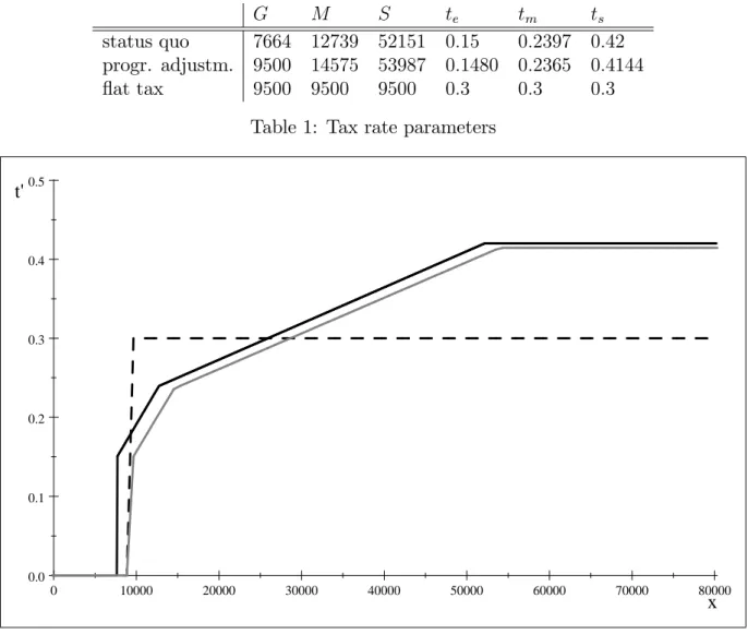
tax rate of the upper progression zone). To ensure revenue neutrality in combination with tax simpli…cation, we adjust the rate schedule to the right (progressive adjustment) on the one hand and we introduce a ‡at tax rate of 30% on the other hand. The parameters for the reform scenarios can be found in table 1. A graphical comparison of the di¤erent tari¤s can be found in …gure 1.

G M S te tm ts

status quo 7664 12739 52151 0:15 0:2397 0:42

progr. adjustm. 9500 14575 53987 0:1480 0:2365 0:4144

‡at tax 9500 9500 9500 0:3 0:3 0:3

Table 1: Tax rate parameters

0 10000 20000 30000 40000 50000 60000 70000 80000 0.0 0.1 0.2 0.3 0.4 0.5 x t'

Figure 1: Marginal tax rates

All scenarios and the corresponding …scal e¤ects are presented in table 7 in the appendix. The simulated measures are separated into two categories: measures concerning the determ-ination of earnings (category A) and those concerning the calculation of the taxable income (category B). First, we analyse the segregated e¤ects on these measures of tax simpli…cation be-fore we examine joint e¤ects of combined measures. Subsequently, we take the abe-forementioned tax rate decreases into account which allows us to model the complete reform with revenue neutrality. For the latter, the distributional e¤ects are also simulated.

Concerning the determination of earnings (category A), we focus on labour income related expenses. According to § 19 EStG (German income tax law) labour income consists of gross wages minus related expenses; there is a lump sum amount of 920e unless higher expenses can be claimed. An integral part of these expenses are commuting costs. The applicable law allows for a deduction of 0,3e per kilometer. Furthermore, we examine the abolition of tax

free bonuses for night, weekend and holiday labour. Concerning capital income we look at the reduction and abolition of the saver‘s allowance (Sparerfreibetrag: current system 1370e for a single, 2740e for a couple household).

In category B, we look at several tax allowances for age, single parents, children12 and deductions for tax accountancy costs, church tax and donations (charitable and for political parties).

4

Complexity of the tax system

We start analysing the e¤ects of tax simpli…cation by asking whether there is an impact of the measures described in the preceding section on the use of professional tax advice, which, following Gale and Rohaly (2003), may be considered as an indicator of both the complexity of the tax system and the compliance costs. Although using this indicator is certainly not without problems, it has the advantage of being “simple and straightforward”13 and it o¤ers evidence on the tax payer’s perception of the complexity of the tax system.

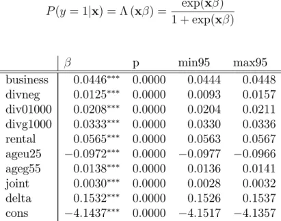
We estimate a logistic regression equation to explain the probability of using a tax consultant (y= 1) depending on various factors x like net income, gross income, income sources and age:

P(y= 1_jx) = (x ) = exp(x ) 1 + exp(x ) p min95 max95 business 0:0446 0:0000 0:0444 0:0448 divneg 0:0125 0:0000 0:0093 0:0157 div01000 0:0208 0:0000 0:0204 0:0211 divg1000 0:0333 0:0000 0:0330 0:0336 rental 0:0565 0:0000 0:0563 0:0567 ageu25 0:0972 0:0000 0:0977 0:0966 ageg55 0:0138 0:0000 0:0136 0:0141 joint 0:0030 0:0000 0:0028 0:0032 delta 0:1532 0:0000 0:1526 0:1537 cons 4:1437 0:0000 4:1517 4:1357

Table 2: Regression on the use of tax consultants

Source: own calculations based on FiFoSiM. indicate signi…cance at the 1% level.

The estimation results for the coe¢ cients are presented in table 2. DELTA is the di¤erence between gross income and taxable income measuring the level of deductions. The higher these

12_{Child bene…ts are still paid.}

deductions are the higher the probability of using a tax consultant. The other variables are dummies interacted with the log of gross income. The presence of business income (BUSINESS), income from dividends or interests (in three categories: DIVNEG (<0), DIV01000 (0<DIV< 1000), DIVG1000 ( 1000)) or income from rent or leasing (RENTAL) have positive e¤ects on the probability. Joint …ling (JOINT) and age (AGEG55) also have a positive impact, while tax payers under 25 (AGEU25) use tax consultants less frequently.

E06 kumA kumB kumAB

P(y= 1_jx) 19:5 18:8 19:1 18:3

costs (bill. e) 1:668 1:602 1:610 1:530

Table 3: Probability of using a tax consultant

Source: own calculations based on FiFoSiM

Using these estimates we predict the probability of using a tax consultant and the expected aggregated national costs of tax consulting for di¤erent reform scenarios. Table 3 reports the results. In the data for the current tax system19:5% of the tax payers use a consultant which results in costs of 1:668 billion euros. The measures modelled here reduce this probability signi…cantly and hence lead to a less complex tax system. The abolition of several tax rule exemptions in category A (determination of adjusted gross income) reduces the probability for the usage of a tax consultant by 0:7 percentage points and the costs by 66 million euros, in category B (calculation of taxable income) by 0:4 percentage points or 58 million, and both bundles combined by 1:2 percentage points, i.e. approximately six percent, and138 million or

8:3percent.

5

Distributional e¤ects

The introduction of a revenue neutral tax reform always yields winners and loosers. To analyse the distributional e¤ects of di¤erent reform scenarios we compute di¤erent distributional meas-ures based on equivalenced household net incomes14. Furthermore, as an innovative element of our analysis, we estimate the polarisation e¤ects of each alternative. Distributional measures have been widely used in simulation studies15_{, whereas polarisation measures have been seldom}

respectively never used in microsimulations (for Germany)16_{. Generally speaking, polarisation} 14_{We use the OECD-scale which weights the household head with a factor of 1, household members over the} age of 15 with 0.5, and under 15 with 0.3. The households net income is divided by the sum of the individual weights of each member (=equivalence factor) to compute the equivalence weighted household income.

15_{Peichl (2005) presents a survey.}

16_{The measurement of polarisation was introduced by Wolfson (1994) and Esteban and Ray (1994) to analyse} the phenomenon of the “declining middle class“ in the United States which could not be satisfactorily explained by standard inequality measures (see Schmidt (2004) for a survey). The distinction between inequality and

is the occurrence of two antipodes. A rising income polarisation describes the phenomenon of a declining middle class resulting in an increasing gap between rich and poor. The proportion of middle income households is declining while the shares of the poor and the rich are both rising. We compute the Gini coe¢ cient17 as a distributional measure and the polarisation index of Schmidt (2004)18. The main results are presented in table 4. We simulate the percentage changes of the mean income in each decile and of the distributional and polarisation indices compared to the status-quo for each tax rate schedule adjustment, the simpli…cation bundle19

and the combinations of rate schedule reforms and tax base simpli…cation.

simpli…cation schedule adj. combinations kumAB progr. ‡at rate progr. ‡at rate 1. Decile -0,01 0,00 0,00 -0,01 -0,01 2. Decile -0,12 0,05 0,04 -0,03 -0,06 3. Decile -0,67 0,95 0,39 0,50 -0,22 4. Decile -1,06 1,76 0,02 0,90 -1,11 5. Decile -1,31 2,14 -0,48 0,99 -1,90 6. Decile -1,47 2,36 -0,91 1,02 -2,49 7. Decile -1,60 2,48 -1,09 0,97 -2,78 8. Decile -1,57 2,69 -0,83 0,99 -2,61 9. Decile -1,57 2,98 -0,02 0,91 -1,96 10. Decile -1,72 2,12 6,32 -0,04 4,68 Gini -0,38 0,48 2,86 -0,21 2,54 PolS -0,98 0,91 -0,56 -0,09 -1,69 P 90/10 -1,65 3,05 0,63 0,78 -1,36 Table 4: Percentage change of household equivalence weighted net income

Source: own calculations based on FiFoSiM

The …rst column of table 4 shows the cumulated e¤ects of the simpli…cation bundle (ku-mAB). The accumulated measures of tax simpli…cation burden the higher incomes more heavily than the middle and the lower incomes. Inequality and polarisation are both reduced. The

polarisation can be vividly explained using the extremes: minimal inequality and minimal polarisation is given by a uniform distribution of income, that is everybody has the same income. Maximal inequality is given if N 1 people realize a zero income and the remaining person receives the whole income. Polarisation is maximal if there are two (almost identically large) groups which are very heterogeneous regarding their incomes (heterogeneity between groups) but very homogeneous inside each group (homogeneity within groups). Put it another way: polarisation considers the relative importance of the middle class while inequality looks at the distribution of the incomes of the individual agents.

17_{Cf. Cowell (1995) for a textbook presentation of the Gini index.}

18_{Schmidt (2004) creates a polarisation index which in analogy to the gini index (lorenz curve) is based on} a polarisation curve for a better comparability of the results and their interpretations.

19_{The complete simpli…cation bundle (kumAB) consists of bundles A (kumA) and B (kumB). All category} B measures of table 7 are combined in bundle B, bundle A contains the abolition of deductibility of commuting costs (A1: noKm), the abolition of the saver’s allowance (Sparerfreibetrag, A4: noSpfb) and the restriction of labour income related expenses to 1000e(A8: wk…x).

separate examination of each bundle yields the same qualitative results.20 _{The abolition of}

sev-eral tax rule exemptions in both categories A (determination of adjusted gross income) and B (calculation of taxable income) a¤ects the high incomes more than the middle and low incomes. The isolated e¤ects of changes in the tax schedule are as follows. The adjustment to the right of the current schedule (column 2) increases inequality as well as polarisation. The ‡at rate tax strongly increases inequality while the polarisation index decreases. The obvious winner of a ‡at tax rate is the 10th decile due to lower statutory and e¤ective marginal rates and to some extent the …rst deciles while the middle to upper deciles su¤er from an increased tax charge due to the ‡at tax reform. These e¤ects result in an overall increase in the Gini index. The decrease in polarisation is surprising at …rst glance, but this result can be attributed to the following two e¤ects: The heterogeneity between the two groups decreases because of the higher tax burden for most people above the median income and because of a decrease of the tax liability of some people below the median. The homogeneity within the upper group decreases as well because of the opposite directions of the e¤ects in those deciles. Both e¤ects lead to a decrease in the polarisation index. The increase of the polarisation index for the adjusted current schedule can be explained by the relatively larger relief for people above the median income resulting in an increasing heterogeneity between the two groups.

The revenue neutral combination of the tax base simpli…cation bundle with a tax schedule adjustment to the right (column 4) decreases both the inequality and the polarisation indices, whereas the combination with a ‡at-tax (column 5) increases the inequality but reduces the polarisation. The explanation is analogous to the e¤ects of the pure tari¤ reforms. Given these results, we can conclude that revenue neutral tax simpli…cation does not necessarily lead to redistribution from poor to rich. The combination with the adjustment of the current tax schedule even leads to a decrease of inequality, i.e. the simpli…cation of the tax system can lead to a more equal distribution of after tax income. More inequality only arises if tax base simpli…cation is combined with the introduction of a ‡at rate tax.

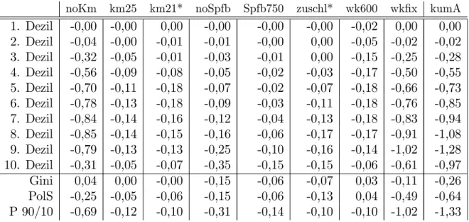
The distributional e¤ects of the single simpli…cation measures are described in the appendix and yield some interesting results.21 _{The abolition of tax free bonuses for night, weekend and}

holiday labour results in an increase of income equality which seems to be counter-intuitive. The burden of this simpli…cation particularly a¤ects middle and high incomes. The same results apply to the abolition of the deduction for commuting costs. This measure also burdens middle and higher incomes more heavily than lower income categories.

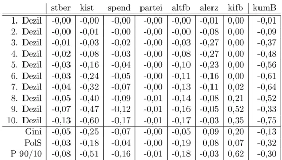
20_{The separated results for each simpli…cation measure can be found in tables 9 and 10.}

21_{Table 8 presents the fractions of the income deciles on the households equivalent weighted net income, the} respective mean income and the upper bound of the decile income. Table 9 contains the simpli…cation measures of category A (determination of adjusted gross income) which would lead to a decrease in both inequality and polarisation. Table 10 presents the results for category B (calculation of taxable income) where both inequality and polarisation decrease.

6

Tax simpli…cation and e¤ective marginal tax rates

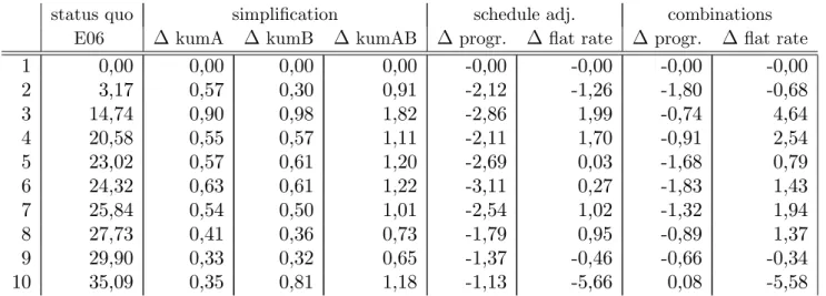
There are many ways in which the simpli…cation of the tax system a¤ects its e¢ ciency. In this section, we analyse the e¤ect of tax simpli…cation on the e¤ective marginal income tax rate faced by di¤erent groups of taxpayers. The underlying idea is that the marginal income tax rate a¤ects the labour supply and savings incentives. Here, we focus on the marginal labour income tax rate. The results are summarised in table 5.

status quo simpli…cation schedule adj. combinations E06 kumA kumB kumAB progr. ‡at rate progr. ‡at rate

1 0,00 0,00 0,00 0,00 -0,00 -0,00 -0,00 -0,00 2 3,17 0,57 0,30 0,91 -2,12 -1,26 -1,80 -0,68 3 14,74 0,90 0,98 1,82 -2,86 1,99 -0,74 4,64 4 20,58 0,55 0,57 1,11 -2,11 1,70 -0,91 2,54 5 23,02 0,57 0,61 1,20 -2,69 0,03 -1,68 0,79 6 24,32 0,63 0,61 1,22 -3,11 0,27 -1,83 1,43 7 25,84 0,54 0,50 1,01 -2,54 1,02 -1,32 1,94 8 27,73 0,41 0,36 0,73 -1,79 0,95 -0,89 1,37 9 29,90 0,33 0,32 0,65 -1,37 -0,46 -0,66 -0,34 10 35,09 0,35 0,81 1,18 -1,13 -5,66 0,08 -5,58

Table 5: Changes in e¤ective marginal tax rates in percentage points

Source: own calculations based on FiFoSiM

It turns out that tax base simpli…cation without tax rate adjustments increases the marginal tax rate for all taxpayers. This is not surprising, given the progressive nature of the income tax schedule. Combining these measures with a reduction of tax rates over the entire income tax schedule reduces the marginal tax rate for almost all taxpayers with the exception of the highest income decile. The combination with a ‡at rate tax, in contrast, reduces the marginal tax rate considerably (by …ve percentage points) for the highest income decile. For the middle income deciles, the marginal tax rate increases, especially for the third and the fourth income decile. This suggests that the e¢ ciency gains that can be achieved through tax simpli…cation, combined with the introduction of a ‡at rate tax, are limited. This is mainly due to the fact that revenue neutrality requires a ‡at tax rate of 30%. If the broadening of the tax base goes beyond the measures considered here, revenue neutrality can be achieved at a lower statutory tax rate. In this case, it would be possible to attain lower marginal tax rates for more households.

7

Labour supply e¤ects

7.1

Model

To analyse the behavioural responses induced by the di¤erent tax reform scenarios we simulate their labour supply e¤ects. Following Van Soest (1995) we apply a discrete choice household labour supply model,22 _{assuming that the household’s head and his partner jointly maximise a}

household utility function in the arguments leisure of both partners and net income. Household

i (i = 1; :::; N) can choose between a …nite number of combinations (yij; lmij; lfij); where

j = 1; :::; J; yij the net income, lmij the leisure of the husband andlfij the leisure of the wife

of householdiin combinationj. Based on our data we choose three working time categories for men (unemployed, employed, overtime) and …ve for women (unemployed, employed, overtime and two part time categories).

We model the following translog23 household utility function

Vij(xij) =x0ijAxij + 0xij (1)

where x = lnyij; lnlmij; lnlfij

0

is the vector of the natural logs of the arguments of the utility function. The elements of x enter the utility function in linear (coe¢ cients

= ( ₁; ₂; ₃)0) and in quadratic and gross terms (coe¢ cients A(3 3) = (aij)). Using control

variables zp (p= 1; :::; P)24 we control for observed heterogeneity in household preferences by

de…ning the parameters _m; mn as

m = XP p=1 mpzp (2) mn = XP p=1 mnpzp (3) where m; n= 1;2;3.

Following McFadden (1973) and his concept of random utility maximisation25 we add a

22_{A detailed description of the FiFoSiM labour supply module can be found in Fuest et al. (2005). A survey} of di¤erent kinds of labour supply models is provided by Blundell and MaCurdy (1999), Creedy et al. (2002) and Hausman (1985) especially for continuous models. Using a discrete choice model has the advantage of the possibility to model nonlinear budget constraints (see Van Soest (1995) or MaCurdy et al. (1990)). Furthermore a discrete choice between distinct categories of working time seems to be more realistic as a continuum of choices because of working time regulations.

23_{Cf. Christensen et al. (1971).}

24_{We use control variables for age, children, region and nationality , which are interacted with the leisure} terms in the utility function because variables without variation across alternatives drop out of the estimation in the conditional logit model (see Train (2003)).

stochastic error term "ij for unobserved factors to the household utility function:

Uij(xij) = Vij(xij) +"ij (4)

= x0_ijAxij + 0xij +"ij

Assuming joint maximisation of the households utility function implies that household i

chooses category k if the utility index of category k exceeds the utility index of any other category l _{2 f}1; :::; J_gnfk_g, if Uik > Uil. This discrete choice modelling of the labour supply

decision uses the probability of ito choose k relative to any other alternative l:

P (Uik > Uil) =P [(x0ikAxik+ 0xik) (x0ilAxil+ 0xil)> "il "ik] (5)

Assuming that "ij are independently and identical distributed across all categories j to

an Gumbel (extreme value) distribution, the di¤erence of the utility index between any two categories follows a logistic distribution. This distributional assumption implies that the prob-ability of choosing alternative k _{2 f}1; :::; J_g for household i can be described by a conditional logit model26_: P (Uik > Uil) = exp (Vik) XJ l=1exp (Vil) (6) = exp (x 0 ikAxik+ 0xik) XJ l=1exp (x 0 ilAxil+ 0xil)

For the maximum likelihood estimation of the coe¢ cients we assume that the hourly wage is constant across the working hour categories and does not depend on the actual working time.27 _{For unemployed people we estimate their (possible) hourly wages by using the Heckman}

correction for sample selection28_{. The household net incomes for each working time category}

are computed in the microsimulation module of FiFoSiM.

7.2

Results

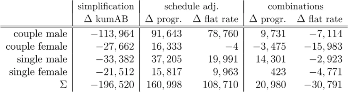
Table 6 contains the full time equivalents of new jobs created as results of our labour supply estimations.

The higher tax burden due to tax base simpli…cation leads to a decrease of labour supply,

26_{McFadden (1973). Cf. Greene (2003) or Train (2003) for textbook presentations.} 27_{Cf. Van Soest and Das (2001).}

28_{Cf. Heckman (1976) and Heckman (1979). A detailed description of these estimations can be found in} Fuest et al. (2005).

simpli…cation schedule adj. combinations kumAB progr. ‡at rate progr. ‡at rate

couple male 113;964 91;643 78;760 9;731 7;114

couple female 27;662 16;333 4 3;475 15;983

single male 33;382 37;205 19;991 14;301 2;923

single female 21;512 15;817 9;963 423 4;771 196;520 160;998 108;710 20;980 30;791

Table 6: Full time equivalents

while the relief of the tax payers due to the schedule adjustments increases the labour supply. The e¤ect for the ‡at rate tax is weaker than that of the progressive adjustment. The combin-ation of simpli…ccombin-ation and schedule adjustment yield two ambiguous results. The combincombin-ation with the progressive adjustment increases labour supply by 21,000 full time equivalents while the revenue-neutral combination with a ‡at tax decreases the labour supply by 30,800. In both cases, the overall e¤ects on labour supply are thus rather small.

8

Summary and conclusion

In this paper, we have examined the e¤ects of tax simpli…cation on the use of professional tax advice, the income distribution, measured by the Gini coe¢ cient and a polarisation index, e¤ective marginal income tax rates, and labour supply. The analysis is based on a behavioural microsimulation model for the German tax and transfer system (FiFoSiM). All e¤ects were simulated for each single simpli…cation measure, for bundles A (determination of earnings) and B (computation of taxable income) and for the complete simpli…cation package. The abolition of tax exemptions increases tax revenue. Therefore our tax simpli…cation package was combined with tax rate reforms to analyse the joint e¤ects on distribution while controlling for revenue neutrality.

The main results are:

Tax base simpli…cation reduces the use of professional tax advice, which can be seen as an indicator of both the complexity of the tax system and the compliance costs, by approximately six per cent.

Tax simpli…cation concerning the determination of income for tax purposes (cat. A) reduces inequality and polarisation. Simplifying the determination of taxable income (cat. B) also reduces inequality and polarisation.

Simpli…cation through the abolition of tax exemptions increases tax revenue. A tax re-form with overall revenue neutrality implies tax rate changes with separate distributional e¤ects.

The adjustment of the current schedule to the right slightly increases inequality and polar-isation while a ‡at tax leads to a distinct increase of inequality and decreases polarpolar-isation.

The combination of a progressive tax rate adjustment and simpli…cation reduces inequality and polarisation, because the highest incomes su¤er most. The marginal income tax rate for middle income households is also reduced. Labour supply increases.

If the simpli…cation package is combined with a ‡at rate tax, inequality increases while polarisation decreases, as the upper middle class is particularly a¤ected. Hence, the tax rate e¤ect is stronger than the simpli…cation e¤ects on distribution and labour supply incentives of middle income households. Labour supply decreases.

Summing up, revenue neutral tax simpli…cation can increase or decrease inequality depend-ing on the form of rate schedule adjustment. Tax simpli…cation in combination with a directly progressive tax rate schedule can reduce inequality. If inequality is regarded as an indicator for fair taxation, more fairness through tax simpli…cation is possible.

Furthermore, our results suggest that ‡at tax reforms combining tax base broadening with a single tax rate are likely to increase inequality at the expense of the upper middle class. This might be the reason for the limited success of ‡at tax proposals in the political process in Germany. Given this, it seems advisable to separate the tax base simpli…cation objective from tax rate schedule issues.

Finally, income distribution is only one relevant aspect of tax reforms. If a higher national income, more e¢ ciency or better incentives can be achieved through an income tax reform, higher inequality of income distribution might be deemed acceptable. Our results suggest that the e¤ects of a ‡at tax rate reform on e¢ ciency in terms of e¤ective marginal tax rates or labour supply are rather limited. However, it should be emphasized that a ‡at rate tax is likely to reduce tax distortions in the corporate sector. This may lead to e¢ ciency gains due to more investment and labour demand.

To conclude, one can state that whether tax simpli…cation leads to more fairness in terms of higher after-tax income equality depends on the simpli…cation method. The tax base simpli-…cation package considered here, combined with an adjusted direct progressive tax rate reduces the inequality of income distribution and increases labour supply while maintaining revenue neutrality. In this regard, more equity and e¢ cency through tax simpli…cation is possible.

Appendix

abbr. income tax solid. tax P

applicable law 2006 E061 180;97 9;95 190;93

tax rate 1 (progressive adjustment) tarif1 12;35 0;68 13;03

tax rate 2 (‡at tax) tarif2 11;53 0;63 12;16

A simpli…cation cat. A (earnings)

A1 abolition commuting costs allowance noKm 4;29 0;24 4;53

A2 reduction commuting costs allowance 0,25e/km km25 0;70 0;04 0;74

A3* commuting costs allowance starting with km 21 km21 1;34 0;07 1;41

A4 abolition of the saver‘s allowance noSpfb 1;50 0;08 1;58

A5 reduction of the saver‘s allowance to 750e Spfb750 0;61 0;03 0;64

A6* abolition of tax free bonuses zuschl 1;34 0;07 1;41

A7 reduction labour income expenses to 600e wk600 1;02 0;06 1;07

A8 labour income expenses restricted to 1000e wk…x 5;13 0;28 5;41

A accumulated (A1, A4, A8) kumA 6;64 0;36 7;00

B simpli…cation cat. B (taxable income)

B1 no deduction of tax accountancy costs noStber 0;53 0;03 0;56

B2 no deduction of church tax noKist 2;86 0;16 3;02

B3 no deduction of charitable donations noSpend 0;79 0;04 0;83

B4 no deduction of donations for political parties noPartei 0;05 0;00 0;05

B5 no age allowance noAltfb 0;67 0;04 0;71

B6 no tax allowance for single parents noAllein 0;85 0;05 0;90

B7 no tax allowance for children noKifb 0;55 0;03 0;58

B accumulated kumB 6;30 0;35 6;65

A, B accumulated kumAB 13;07 0;72 13;79

A, B accumulated with tax rate 1 (new) kumAB1 0;00 0;00 0;00

A, B accumulated with tax rate 2 (‡at) kumAB2 0;01 0;00 0;01

Table 7: Scenarios and …scal e¤ects in billione

decile fraction accumulated mean cutpoint 1 0,88 0,88 1.764,33 4.179,38 2 3,35 4,23 6.746,41 9.019,61 3 5,32 9,55 10.699,30 12.172,71 4 6,66 16,21 13.390,84 14.543,69 5 7,79 23,99 15.658,02 16.756,27 6 8,88 32,88 17.869,07 19.010,10 7 10,09 42,97 20.296,47 21.703,05 8 11,67 54,64 23.474,42 25.549,16 9 14,28 68,92 28.726,24 32.941,36 10 31,08 100,00 62.504,63 . Table 8: Deciles of weighted equivalent net incomes

Source: own calculations based on FiFoSiM.

noKm km25 km21* noSpfb Spfb750 zuschl* wk600 wk…x kumA

1. Dezil -0,00 -0,00 0,00 -0,00 -0,00 -0,00 -0,02 0,00 0,00 2. Dezil -0,04 -0,00 -0,01 -0,01 -0,00 0,00 -0,05 -0,02 -0,02 3. Dezil -0,32 -0,05 -0,01 -0,03 -0,01 0,00 -0,15 -0,25 -0,28 4. Dezil -0,56 -0,09 -0,08 -0,05 -0,02 -0,03 -0,17 -0,50 -0,55 5. Dezil -0,70 -0,11 -0,18 -0,07 -0,02 -0,07 -0,18 -0,66 -0,73 6. Dezil -0,78 -0,13 -0,18 -0,09 -0,03 -0,11 -0,18 -0,76 -0,85 7. Dezil -0,84 -0,14 -0,16 -0,12 -0,04 -0,13 -0,18 -0,83 -0,94 8. Dezil -0,85 -0,14 -0,15 -0,16 -0,06 -0,17 -0,17 -0,91 -1,08 9. Dezil -0,79 -0,13 -0,13 -0,25 -0,10 -0,16 -0,14 -1,02 -1,28 10. Dezil -0,31 -0,05 -0,07 -0,35 -0,15 -0,15 -0,06 -0,61 -0,97 Gini 0,04 0,00 -0,00 -0,15 -0,06 -0,07 0,03 -0,11 -0,26 PolS -0,25 -0,05 -0,06 -0,15 -0,06 -0,13 0,04 -0,49 -0,64 P 90/10 -0,69 -0,12 -0,10 -0,31 -0,14 -0,10 -0,10 -1,02 -1,33

Table 9: Percentage changes of net income in cat. A.

stber kist spend partei altfb alerz kifb kumB 1. Dezil -0,00 -0,00 -0,00 -0,00 -0,00 -0,01 0,00 -0,01 2. Dezil -0,00 -0,01 -0,00 -0,00 -0,00 -0,08 0,00 -0,09 3. Dezil -0,01 -0,03 -0,02 -0,00 -0,03 -0,27 0,00 -0,37 4. Dezil -0,02 -0,08 -0,03 -0,00 -0,08 -0,27 0,00 -0,48 5. Dezil -0,03 -0,16 -0,04 -0,00 -0,10 -0,23 0,00 -0,56 6. Dezil -0,03 -0,24 -0,05 -0,00 -0,11 -0,16 0,00 -0,61 7. Dezil -0,04 -0,32 -0,07 -0,00 -0,13 -0,11 0,02 -0,64 8. Dezil -0,05 -0,40 -0,09 -0,01 -0,14 -0,08 0,21 -0,52 9. Dezil -0,07 -0,47 -0,12 -0,01 -0,16 -0,05 0,52 -0,33 10. Dezil -0,13 -0,60 -0,17 -0,01 -0,17 -0,03 0,35 -0,75 Gini -0,05 -0,25 -0,07 -0,00 -0,05 0,09 0,20 -0,13 PolS -0,03 -0,18 -0,04 -0,00 -0,19 0,08 0,07 -0,32 P 90/10 -0,08 -0,51 -0,16 -0,01 -0,18 -0,03 0,62 -0,30

Table 10: Percentage changes of net income in cat. B.

Source: own calculations based on FiFoSiM.

References

Blundell, R. and MaCurdy, T. (1999). Labor Supply: A Review of Alternative Approaches,

in O. Ashenfelter and D. Card (eds), Handbook of Labor Economics, Vol. 3A, Elsevier, pp. 1559–1695.

Christensen, L., Jorgenson, D. and Lau, L. (1971). Conjugate Duality and the Transcedental Logarithmic Function, Econometrica 39: 255–256.

Cowell, F. A. (1995). Measuring Inequality, Prentice-Hall, Hemel Hempstead.

Creedy, J., Duncan, A., Harris, M. and Scutella, R. (2002). Microsimulation Modelling of Taxation and the Labour Market: the Melbourne Institute Tax and Transfer Simulator, Edward Elgar Publishing, Cheltenham.

Esteban, J. and Ray, D. (1994). On the Measurement of Polarization,Econometrica62(4): 819– 851.

Fuest, C., Peichl, A. and Schaefer, T. (2005). Dokumentation FiFoSiM: Integriertes Steuer-Transfer-Mikrosimulations- und CGE-Modell, Finanzwissenschaftliche Diskus-sionsbeiträge Nr. 05 - 03.

Fuest, C., Peichl, A. and Schaefer, T. (2006 (forthcoming)). Führt Steuervereinfachung zu einer "gerechteren" Einkommensverteilung? Eine empirische Analyse für Deutschland,

Gale, W. (2001). Tax Simpli…cation: Issues and Options, mimeo.

Gale, W. G., Houser, S. and Scholz, J. K. (1996). Distributional E¤ects of Fundamental Tax Reform, in H. J. Aaron and W. G. Gale (eds), Economic E¤ects of Fundamental Tax Reform, The Brookings Institution, Washington, D. C., pp. 281–320.

Gale, W. and Rohaly, J. (2003). E¤ects of Tax Simpli…cation Options on Equity, E¢ ciency, and Simplicity: A Quantitative Analysis.

Greene, W. (2003). Econometric Analysis, Prentice Hall, New Jersey.

Gupta, A. and Kapur, V. (2000). Microsimulation in Government Policy and Forecasting, North-Holland, Amsterdam.

Haisken De-New, J. and Frick, J. (2003). DTC - Desktop Compendium to The German Socio-Economic Panel Study (GSOEP).

Hall, R. E. and Rabushka, A. (1995).The Flat Tax, 2nd edn, Hoover Institution Press, Stanford.

Harding, A. (1996). Microsimulation and public policy, North-Holland, Elsevier, Amsterdam.

Hausman, J. (1985). Taxes and Labor Supply,inA. Auerbach and M. Feldstein (eds),Handbook of Public Economics, North-Holland, Amsterdam, pp. 213–263.

Heckman, J. (1976). The Common Structure of Statistical Models of Truncation, Sample Selection and Limited Dependent Variables and a Simple Estimator for Such Models,

Annals of Economic and Social Measurement 5: 475–492.

Heckman, J. (1979). Sample Selection Bias as a Speci…cation Error,Econometrica47: 153–161.

James, S., Sawyer, A. and Wallschutzky, I. (1997). Tax Simpli…cations: A Tale of Three Countries, Bulletin for International Fiscal Documentation51: 493–503.

Kirchhof, P., Altehoefer, K., Arndt, H.-W., Bareis, P., Eckmann, G., Freudenberg, R., Hahnemann, M., Kopei, D., Lang, F., Lückhardt, J. and Schutter, E. (2001). Karlsruher Entwurf zur Reform des Einkommensteuergesetzes, http://www.uni-heidelberg.de/institute/fak2/kirchhof/estg-entwurf.pdf.

MaCurdy, T., Green, D. and Paarsch, H. (1990). Assessing Empirical Approaches for Analyzing Taxes and Labor Supply,Journal of Human Resources 25(3): 415–490.

McFadden, D. (1973). Conditional Logit Analysis of Qualitative Choice Behaviour, in P. Za-rembka (ed.),Frontiers in Econometrics, New York, pp. 105–142.

McFadden, D. (1981). Econometric Models of Probabilistic Choice, in C. Manski and D. Mc-Fadden (eds), Structural Analysis of Discrete Data and Econometric Applications, The MIT Press, Cambridge, pp. 198–272.

McFadden, D. (1985). Econometric Analysis of Qualitative Response Models, in Z. Griliches and M. Intrilligator (eds), Handbook of Econometrics, Elsevier, Amsterdam, pp. 1396– 1456.

Merz, J., Vorgrimler, D. and Zwick, M. (2005). De facto anonymised microdata …le on income tax statistics 1998, FDZ-Arbeitspapier Nr. 5.

O’Hare, J. and Gupta, A. (2000). Practical Aspects of Microsimulation Modelling,inA. Gupta and V. Kapur (eds), Microsimulation in Government Policy and Forecasting, North-Holland, Amsterdam, pp. 563–640.

Peichl, A. (2005). Die Evaluation von Steuerreformen durch Simulationsmodelle, Finanzwis-senschaftliche Diskussionsbeiträge Nr. 05-01, Universität Köln.

Rässler, S. (2002). Statistical Matching, Springer, New York [u.a.].

Schmidt, A. (2004). Statistische Messung der Einkommenspolarisation, Eul-Verlag, Lohmar.

Slemrod, J. (1984). Optimal tax Simpli…cation - Toward a Framework for Analysis,Proceedings of the Seventy-Sixth Annual Conference on Taxation - National Tax Association - Tax Institute of America pp. 158–167.

Slemrod, J. (1992). Did the Tax Reform Act of 1986 Simplify Tax Matters?, Journal of Eco-nomic Perspectives 6: 45–57.

Train, K. (2003). Discrete Choice Models Using Simulation, Cambridge University Press, Cam-bridge.

Tran-Nam, B. (2000). Tax Reform and Tax Simplicity: A New and "Simpler" Tax System?,

UNSW Law Journal 23: 241–251.

Van Soest, A. (1995). Structural Models of Family Labor Supply: A Discrete Choice Approach,

Journal of Human Resources30: 63–88.

Van Soest, A. and Das, M. (2001). Family Labor Supply and Proposed Tax Reforms in the Netherlands, De Economist 149(2): 191–218.

Wagenhals, G. (2001). Incentive and Redistribution E¤ects of the Karlsruher Entwurf zur Reform des Einkommenssteuergesetzes, Schmollers Jahrbuch 4: 425–437.

Wagenhals, G. (2004). Tax-bene…t microsimulation models for Germany: A Survey, IAW-Report / Institut fuer Angewandte Wirtschaftsforschung (Tübingen) 32(1): 55–74.

Wagner, F. (2006). Was bedeutet Steuervereinfachung wirklich?, Perspektiven der Wirtschaft-spolitik7: 19–33.

F

D

Eine Schriftenreihe des Finanzwissenschaftlichen Forschungsinstituts an der Universität zu Köln

ISSN 0945-490X

Die Beiträge ab 1998 (z.T. auch ältere) stehen auch als kostenloser Download (pdf) zur Verfügung unter: http://www.fifo-koeln.de

1993

93-1 Ewringmann, D.: Ökologische Steu-erreform? Vergriffen

93-2 Gawel, E.:

Bundesergänzungszu-weisungen als Instrument eines rati-onalen Finanzausgleichs. Vergriffen

93-3 Ewringmann, D. / Gawel, E. /

Hans-meyer, K.-H.: Die Abwasserabgabe

vor der vierten Novelle: Abschied vom gewässergütepolitischen Len-kungs- und Anreizinstrument, 2. Aufl. Vergriffen

93-4 Gawel, E.: Neuere Entwicklungen der Umweltökonomik. Vergriffen

93-5 Gawel, E.: Marktliche und außer-marktliche Allokation in staatlich re-gulierten Umweltmedien: Das Prob-lem der Primärallokation durch Recht. Vergriffen

1994

94-1 Gawel, E.: Staatliche Steuerung durch Umweltverwaltungsrecht — eine ökonomische Analyse. Vergriffen

94-2 Gawel, E.: Zur Neuen Politischen Ökonomie der Umweltabgabe. Ver-griffen

94-3 Bizer, K. / Scholl, R.: Der Beitrag der

Indirekteinleiterabgabe zur Reinhal-tung von Klärschlamm.Vergriffen

94-4 Bizer, K.: Flächenbesteuerung mit

ökologischen Lenkungswirkungen.

Vergriffen 1995

95-1 Scholl, R.: Verhaltensanreize der Ab-wasserabgabe: eine Untersuchung der Tarifstruktur der Abwasserabga-be. ISBN 3-923342-39-X. 6,50 EUR

95-2 Kitterer, W: Intergenerative Belas-tungsrechnungen („Generational Accounting“) - Ein Maßstab für die Belastung zukünftiger Generatio-nen? ISBN 3-923342-40-3. 7,50 EUR

1996

96-1 Ewringmann, D. / Linscheidt, B. /

Truger, A.: Nationale

Energiebe-steuerung : Ausgestaltung und

Auf-kommensverwendung. ISBN

3-923342-41-1.10,00 EUR

96-2 Ewringmann, D. / Scholl. R.: Zur fünften Novellierung der Abwasser-abgabe; Meßlösung und sonst nichts? ISBN 3-923342-42-1. 7,50 EUR

1997

97-1 Braun, St. / Kambeck, R.: Reform der Einkommensteuer. Neugestaltung des Steuertarifs. ISBN

3-923342-43-8. 7,50 EUR

97-2 Linscheidt, B. / Linnemann, L.: Wir-kungen einer ökologischen Steuerre-form – eine vergleichende Analyse der Modellsimulationen von DIW und RWI. ISBN 3-923342-44-6. 5,00 EUR

97-3 Bizer, K. / Joeris, D.: Bodenrichtwerte als Bemessungsgrundlage für eine reformierte Grundsteuer. ISBN 3-923342-45-4, 7,50 EUR

1998

98-1 Kitterer, W.: Langfristige Wirkungen

öffentlicher Investitionen - theoreti-sche und empiritheoreti-sche Aspekte. ISBN 3-923342-46-2. 6,00 EUR

98-2 Rhee, P.-W.: Fiskale Illusion und

Glo-ry Seeking am Beispiel Koreas (1960-1987). ISBN 3-923342-47-0. 5,00 EUR

98-3 Bizer, K.: A land use tax: greening the

property tax system. ISBN 3-923342-48-9. 5,00 EUR

2000

00-1 Thöne, M.: Ein Selbstbehalt im

Län-derfinanzausgleich?. ISBN 3-923342-49-7. 6,00 EUR

00-2 Braun, S., Kitterer, W.: Umwelt-, Beschäftigungs- und Wohlfahrtswir-kungen einer ökologischen Steuerre-form : eine dynamische Simulations-analyse unter besonderer Berück-sichtigung der Anpassungsprozesse im Übergang. ISBN 3-923342-50-0. 7,50 EUR

2002

02-1 Kitterer, W.: Die Ausgestaltung der Mittelzuweisungen im Solidarpakt II. ISBN 3-923342-51-9. 5,00 EUR

2005

05-1 Peichl, A.: Die Evaluation von

Steuer-reformen durch Simulationsmodelle ISBN 3-923342-52-7. 8,00 EUR

05-2 Heilmann, S.: Abgaben- und

Mengen-lösungen im Klimaschutz : die In-teraktion von europäischem Emissi-onshandel und deutscher Ökosteuer. ISBN 3-923342-53-5. 8,00 EUR

05-3 Fuest, C., Peichl, A., Schaefer, T.: Do-kumentation FiFoSiM: Integriertes Steuer-Transfer-Mikrosimulations- und CGE-Modell. ISBN 3-923342-54-3. 8,00 EUR

2006

06-1 Fuest, C., Peichl, A., Schaefer, T.:

Führt Steuervereinfachung zu einer „gerechteren“ Einkommensvertei-lung? Eine empirische Analyse für Deutschland. ISBN 3-923342-55-1. 6,00 EUR.

06-2 Bergs, C., Peichl, A.: Numerische

Gleichgewichtsmodelle - Grundla-gen und Anwendungsgebiete. ISBN 3-923342-56-X. 6,00 EUR.

06-3 Thöne, M.: Eine neue Grundsteuer –

Nur Anhängsel der Gemeindesteu-erreform? ISBN 3-923342-57-8. 6,00 EUR.

06-4 Mackscheidt, K.: Über die

Leistungs-kurve und die Besoldungsentwick-lung im Laufe des Lebens. ISBN 3-923342-58-6. 6,00 EUR