Active and Adaptive Techniques for Learning over Large-Scale Graphs

(1)

Active and Adaptive Techniques for

Learning over Large-Scale Graphs

A DISSERTATION

SUBMITTED TO THE FACULTY OF THE GRADUATE SCHOOL OF THE UNIVERSITY OF MINNESOTA

BY

Dimitrios Bermperidis

IN PARTIAL FULFILLMENT OF THE REQUIREMENTS FOR THE DEGREE OF

DOCTOR OF PHILOSOPHY

Prof. Georgios B. Giannakis, Advisor

(2)

c

(3)

Acknowledgments

Foremost, I would like to express my sincere gratitude to my advisor Prof. Georgios B. Giannakis for giving me the opportunity to be a part of the SPiNCOM research group, as well as the ECE/CS graduate program of University of Minnesota. With his continued guidance and support, he has greatly helped me in taking my first steps into the world of research and engineering, leading to the completion of this thesis. In addition, he has and continues to aid me in developing clear scientific thought and expression.

In a special way I would like to extend my appreciation to Prof. George Karypis, Prof. Zhili Zhang, and Prof. Mingyi Hong who agreed to serve on my thesis committee, and provided with much appreciated feedback that helped improve this work. Thanks go to a number of other professors in the departments of Electrical Engineering and Computer Science whose graduate level courses provided me with the necessary background to embark on this area of research.

Special thanks also go to Prof. Vassilis Kekatos for his help and guidance through the first stages of my PhD. I thank my good friends, companions and collaborators Dr. Fateme Sheik-holeslami, Dr. Donghoon Lee, Vassilis Ioannidis, Panos Traganitis, and Charilao Kanatsoulis. Special thanks to my friend and collaborator Dr. Athanasios Nikolakopoulos for helping me expand my research/technical skills and for donating some of his unlimited enthusiasm to me. I thank all my fellow lab-mates and good friends in SPINCOM for their support and all the fruitful discussions we had over the years.

Last but not the least, I would like to express by deepest thanks to my family: my parents Kostas and Maria, my grand-parents Dimitris, Fevronia, and Xrisanthi, and my dear brother Theodoros for their continued love and support throughout my life.

Dimitris Berberidis, Minneapolis, May 31, 2019.

(4)

Dedication

This dissertation is dedicated to my family.

(5)

Abstract

Behind every complex system be it physical, social, biological, or man-made, there is an intricate network encoding the interactions between its components. Learning over large-scale networks is a challenging field, and practical methods must combinescalabilityin computations to cope with millions of nodes associated possibly with large amounts of meta-information; along with sufficientversatilityto capture the elaborate structure and dynamics of the complex phenomena under study. There is also a need for modelingexpressivenessto ensure accurate learning, along with transparency andinterpretabilitythat will shed light on the overall system understanding, and will provide valuable insights about its function. Approaches to learning over networks must alsodefend against adversarial behavior, thus remaining operational even under severely adverse circumstances.

The contribution of the present thesis lies at addressing the aforementioned challenges by developing simple yet versatile algorithmic solutions focused on core graph-learning tasks. To tackle active sampling for semi-supervised node classification, a novel framework is proposed in order to guide the sampling of informative nodes. The proposed framework is tailored to Gaussian-Markov random fields, and relies on the notion of maximum expected-change to select the most informative node to be labeled. Interestingly, several existing methods for active learning are subsumed by the proposed approach. Focusing on the node classification task, a generalized yet highly scalablediffusion-basedclassifier is developed, where each class diffusion is adaptive to the graph structure and the underlying label distribution. Adaptability is further leveraged for the node embedding task. As node embedding is naturally viewed as a low-rank factorization of a node-to-node similarity matrix, a versatile approach is introduced to learn the similarity matrix of a given graph with minimal computational overhead, and in a fully unsupervised manner. Extensive experimentation using both synthetic graphs as well as numerous real networks demonstrates the effectiveness, interpretability and scalability of the proposed methods. More importantly, the process of design and experimentation sheds light on the behavior of different methods and the peculiarities of real-world data, while at the same time generates new ideas and directions to be explored.

(6)

List of Tables

2.1 Summary of EC methods based on different metrics of change . . . 28

2.2 Computational and memory complexity of various methods . . . 29

2.3 Dataset list . . . 36

3.1 Network Characteristics . . . 59

3.2 Micro F1 and Macro F1 Scores on Multiclass Networks (class-balanced sam-pling) . . . 60

3.3 Micro F1 and Macro F1 Scores of Various Algorithms on Multilabel Networks 60 4.1 Network Characteristics . . . 87

4.2 Inferred parameters and interpretation . . . 87

4.3 Link Prediction Accuracy onvk2016-17 . . . 90

(10)

List of Figures

1.1 Visualization of the 2004 US presidential elections blogosphere graph. Blue nodes correspond to democratic political blogs, while red denotes republican ones. Links correspond to blogs that contain references to each other. The clustering of the graph to a blue and red group indicates the high degree of

polarization that characterizes the US political landscape. . . 5

1.2 Subgraph of the Homo Sapiens protein-protein interaction (PPI) network ex-tracted from theSting Consortiumrepository (link). . . 6

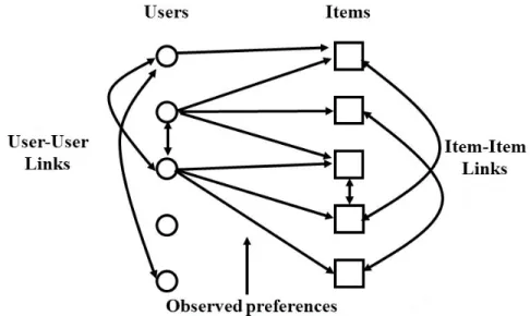
1.3 Graph-based representation of the recommendation setting. Users (round nodes) and items (square nodes) form a heterogeneous network. User-item links are formed from observed user preferences and/or implicit feedback, while (optional) intra-user links may be available from friendships networks, and intra-item links may be inferred from data. . . 7

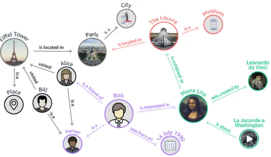
1.4 Example of a knowledge graph constructed fromentity/relation/entity triples. . . 8

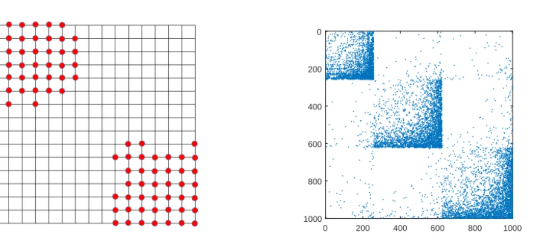
2.1 Rectangular grid synthetic graph with two separate class 1 regions. . . 35

2.2 Adjacency matrix of LFR graph with 1,000 nodes and 3 classes. . . 35

2.3 Test results for synthetic grid in Fig. 1 . . . 35

2.4 Test results for synthetic LFR graph in Fig. 2. . . 35

2.5 Coloncancer dataset. . . 37 2.6 Ionosphere dataset. . . 37 2.7 Leukemia dataset. . . 37 2.8 Australian dataset. . . 37 2.9 Parkinsons dataset. . . 37 2.10 Ecoli dataset. . . 37 viii

(11)

2.12 CITESEER citation network. . . 38 2.13 Political blogs network. . . 38 2.14 Relative runtime of different adaptive methods for experiments on real social

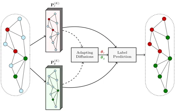
graphs. . . 38 3.1 High-level illustration of adaptive diffusions. The nodes belong to two classes

(redandgreen). The per-class diffusions are learned by exploiting the landing probability spaces produced by random walks rooted at the sample nodes (second layer:upfor red;downfor green). . . 44 3.2 Illustration ofK = 20landing probability coefficients for PPR withα = 0.9,

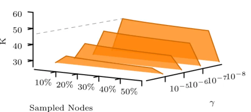
HK witht= 10, and AdaDIF (λ= 15). . . 47 3.3 Experimental evaluationKγfor different values ofγ-distinguishability threshold,

and proportions of sampled nodes onBlogCataloggraph. . . 49 3.4 Micro-F1 score for AdaDIF and non-adaptive diffusions on5%labeledCora

graph as a function of the length of underline random walks. . . 61 3.5 Classification accuracy of AdaDIF, PPR, and HK compared to the accuracy

ofk−step landing probability classifier. First line isCora graph, second is

Citeseer, and third isPubMed. Left column is Micro F1 and right column is Macro F1 score. . . 62 3.6 AdaDIF diffusion coefficients for the50different classes of PPI graph (30%

sampled). Each line corresponds to a differentθc. Diffusion is characterized by high diversity among classes. . . 63 3.7 Relative runtime comparisons for multiclass graphs. . . 64 3.8 Classification accuracy of various diffusion-based classifiers on Cora, as a

func-tion of the probability of label corrupfunc-tion. . . 67 3.9 Anomaly detection performance of r-AdaDIF for different label corruption

probabilities. The horizontal axis corresponds to the frequency with which r-AdaDIF returns a true positive (probability of detection) and the vertical axis corresponds to the frequency of false positives (probability of false alarm). . . . 68 4.1 Depiction of groundtruth and estimated similarity matrices, as yielded from an

instance of the numerical experiments described in Section 4.1.1. . . 93

(12)

4.2 MatrixS is equivalent to applying “wavelet”-type weightsατ(k)over walks with hops≤k. . . 94 4.3 Quality of match between true SBM similarity and various estimates, as yielded

from experiments of Section 4.1.1. . . 95 4.4 Micro and MacroF1scores for the four labeled graphs, when the “pure”k−order

Sk _{is used for embedding, given as a function of} _{k. Red shade denotes the} correspondingk’s where ASE assigned non-zeroθk’s; see also Table 2. . . 96 4.5 Micro (upper row) and Macro (lower row)F1scores that different embeddings

+ logistic regression yield on labeled graphs, as a function of the labeling rated (percentage of training data) . . . 97 4.6 Average conductance of different embeddings used by kmeans for clustering, as

a function of number of clusters. . . 98 4.7 Sensitivity of ASE onPPIgraphs wrt various parameters. . . 99 4.8 Runtime of various embedding methods across different graphs . . . 99

(13)

Chapter 1

Introduction

1.1

Learning over Graphs

In many shapes and forms, networks play a fundamental role in our life. The seamless regulations of genes and metabolites within cells are responsible for our biological existence. The coherent interactions between billions of neurons in our brains enables us to comprehend the world. The social bonds and ties between individuals comprise the fabric of our society. Power networks supply us with energy. Trade networks maintain our ability to exchange goods and services. Communication networks enable and empower the most revolutionary technologies of the 21st century. Behind every complex system there is an intricate network capturing the interactions among its components. Reasoning about these networks is one of the major intellectual and scientific challenges of the 21st century.

Statistical learning over networks comprises a suite of computational tools to address core tasks relevant to a host of applications arising in diverse disciplines. For example, node classifi-cation in protein-protein interaction networks aims to associate proteins with specific biological functions, thereby facilitating the understanding of pathogenic and physiological mechanisms. Link prediction in user-product purchase networks can enable personalized recommendations, as well as targeted content delivery and advertising. Community detection in brain networks can help identify the fundamental structures that control and mediate its information pathways, that also unveil its higher-order connectivity patterns and organization.

Let us begin by shortly introducing the graph, an abstract mathematical concept, and at the same time one of the most intuitive and familiar ways of representing relations between

(14)

interconnected entities. A graph is typically denoted byG ={V,E}, whereV is the set ofN nodes, and E contains the edges. There are several different ways to represent a graph. The

adjacency-listandedge-listformats are most frequently employed for low-level algorithmic de-sign and software implementations since they naturally leverage sparsity, and are more amenable to simple operations such as node exploration (e.g., breadth-first-search using an adjacency list). Nevertheless, for problems that involve higher level abstractions (e.g., spectral clustering) theadjacency matrixformat provides with convenient representation that can exploit the full arsenal of linear algebra tools. Thus, in the machine learning context, graphs are most frequently represented by theN×N(possibly) weighted adjacency matrixAwhose(i, j)−th entry denotes the weight of the edge that connects nodeviwith nodevj.

In many applications, graphs emerge naturally, withV andE readily collected and stored. In other cases, a graph can be inferred from a set ofN nodal (a.k.a. feature) vectors{xi}Ni=1 representing data points, such that each node of the graph corresponds to a data point. Matrix Acan be obtained from the feature vectors{xi}Ni=1 using different similarity measures. For example, one may use the radial basis functionwi,j = exp −kxi−xjk22/σ2

that assigns large edge weights to pairs of points that are neighbors in Euclidean space, or the Pearson correlation coefficientswi,j =hxi,xji/(kxik2kxjk2).. Ifwi,j 6= 0∀i, j, the resulting graph will be fully connected, but one may obtain a more structured graph by thresholding small weights to0, or by connecting every point only with itsk−nearest neighbors.

The unique properties and characteristics of graphs have led to a learning approach that is distinct from the “traditional” one that deals with vectors. Thus, graph-based learning, learning-over-graphs, or graph-mining are often interchangable terms that are frequently used to describe one or more of the following tasks.

• Classification. In many cases, each nodevi is associated with one (or more) discrete label(s)yi∈ Y drawn from a finite alphabet. In this context, the goal of semi-supervised classification amounts to propagating an observed subset of labels{yi}i∈L, whereL ⊆ V,

to the rest of the network, in order to infer the labels{yi}i∈U of the set of unlabeled nodes

U :=V/L.

• Community detection/Clustering. Another typical graph learning task is that of cate-gorizing the nodes of the graph toK overlapping (soft-clustering) or non-overlapping clusters, also known as communities. The communities{C_k}K

(15)

typically inferred in a fullyunsupervisedmanner, that relies only on the graph structure. Given a subset of nodesSk ⊂ Ckthat areknownto belong to thek-th community however, semi-supervised community detection aims at inferring the remaining hidden (latent) members ofC_k– a task that has also been posed and gathered significant research interest.

• Link Prediction/ Node Recommendation.Many real graphs are dynamic in nature, with new links appearing (or disappearing) with time. Link prediction is the task of identifying the patterns according to which new links are formed, and accurately inferring them beforehand. One way to pose the link prediction task is that, given the edgesEtat time t, one would like to determinePr{(vi, vj) ∈ Et+1} ∀(vi, vj) ∈ V × V \ Et; that is, the likelihood that a new potential edge(vi, vj)will be present in the next instanceEt+1of the edge set. Similarly,node recommendationis the task of predicting the links{(vi, vj)}j∈Vi

that a given nodevi is expected (or would “prefer”) to form in a future instance of the graph; andVican thus be recommended tovi as a set of possible connections.

• Node Embedding.Many graph learning tasks can be addressed by first extracting features over the nodes of the graph, effectively “embedding” them in a Eucledian space; the extracted features may then be used by downstream machine learning methods to perform classification, link prediction, clustering, and other tasks. Thus, node embedding boils down to determiningf(·) :V →Rd, wheredN. In other works, a function is sought to map every node ofGto a vector in thed−dimensional Euclidean space. Typically, the embedding is low dimensional withdmuch smaller than the number of nodes. Givenf(·), the low-dimensional vector representation of each nodeviisei=f(vi) ∀vi ∈ V. Since the number of nodes is finite, instead of finding a generalf(·)inductively, one may pose the embedding task in its most general form as a the following minimization problem over the embedded vectors

{e∗_i}N_i₌₁= arg min

{ei}N_i₌₁

X

vi,vj∈V

`(sG(vi, vj), sE(ei,ej)) (1.1) where`(·,·) :R×R→Ris a loss function;sG(·,·) :V × V →Ris a similarity metric

over pairs of graphnodes; andsE(·,·) : Rd×Rd→ Ra similarity metric over pairs of

vectorsin thed−dimensional Euclidean space. In par with (4.1), node embedding can be viewed as the design of nodal vectors{ei}N_i₌₁that successfully “encode” a certain notion

(16)

of pairwise similarities among graph nodes.

1.2

Motivation and Context

Learning-over-graphs is well motivated by a large number of applications. This has led to ever-increasing research efforts in this area during the last two decades. Nevertheless, many real-world issues and practical aspects of the problem face formidable challenges to this day. The main focus of the present work is to identify and address such challenges using simple, robust, and interepretable mathematical and algorithmic tools.

1.2.1 Applications of graph-based learning

In this subsection, we discuss some important and contemporary applications of graph-based learning. The goal here is to demonstrate how graphs naturally emerge in diverse domains, and how learning/mining over such graphs can be instrumental in addressing real-world problems.

Social networks

Social networks is a broad term used to describe the class of naturally-occurring complex networks that arise upon registering the interactions (edges) between a set of social entities or actors (nodes). The nodes in social networks may correspond to individuals, groups of individuals, organizations, products, websites, and many other possible types of interacting entities. Social networks are ubiquitous in the physical world, and even more so in cyberspace. Specifically, the proliferation of Internet connectivity since the start of the 21-st century has given birth to a huge variety of online social networking platforms [1], connecting individuals in many contexts (professional, social, dating, and others). Ease of Internet access has led to several of the social networking platforms (e.g., Facebook, Twitter, Youtube) growing to unprecedented proportions, scaling to billions of nodes, and encompassing a sizeable portion of the human population. The analysis of such networks is of interest both for the increase in profitability, as well as the advancements on our understanding of socials structures that it can offer. A common task is to group individuals to overlapping categories. This may help in identifying underlying characteristics and trends in a given populations; see, for instance, Fig. 1.1 for a depiction of the 2004 political US blogosphere graph during the presidential elections, where liberal and

(17)

Figure 1.1: Visualization of the 2004 US presidential elections blogosphere graph. Blue nodes correspond to democratic political blogs, while red denotes republican ones. Links correspond to blogs that contain references to each other. The clustering of the graph to a blue and red group indicates the high degree of polarization that characterizes the US political landscape.

conservative blogs are clearly separated into two clusters. Furthermore, ascertaining social network nodes as e.g., male or female and conservative or liberal, can in general be treated as clustering in lack of supervision, or classification in the presence of some additional information on a subset of the individuals. For example, given a friendship network, the political preferences of a few individuals, and using the “homophily” assumption, an individual’s political opinion will most likely be aligned with those of close friends, the political opinions of unobserved individuals can be inferred by “association.” Finally, social networking platforms rely heavily on link prediction and node recommendation to expand their networks, and keep their users interested by suggesting the formation of new friendships.

(18)

Figure 1.2: Subgraph of the Homo Sapiens protein-protein interaction (PPI) network extracted from theSting Consortiumrepository (link).

Biological networks

Protein–protein interactions (PPI) networks link proteins according to physical contacts of high specificity established between two or more molecules as a result of biochemical events; see e.g., Fig. 1.2 for a subraph extracted from the Homo Sapiens PPI network. Given a set of functionally uncharacterized genes or proteins from a Genome-Wide Association Study, or differential expression analysis, experimental biologists often have little a priori information available to guide the design of hypothesis-based experiments to determine molecular functions. For example, what is the expected phenotype if a particular gene is removed? It would greatly improve hypothesis formation if biologists had prior insight from predicted functions of interesting genes or proteins in databases. Computational annotation of genes or proteins with unknown functions is thus a fundamental research area in computational biology. From a graph-learning perspective, the task of protein function prediction falls under the category of semi-supervised classification. In this context, diffusion-based network models are widely used for protein function prediction using protein network data, and have been shown to outperform neighborhood-based and module-based methods [63].

(19)

Figure 1.3: Graph-based representation of the recommendation setting. Users (round nodes) and items (square nodes) form a heterogeneous network. User-item links are formed from observed user preferences and/or implicit feedback, while (optional) intra-user links may be available from friendships networks, and intra-item links may be inferred from data.

.

Recommender systems

Top-nrecommendation algorithms provide ranked lists of items tailored to the particular user-specific preferences, as depicted by their past interactions. Over the past years, they have become an indispensable component of most e-commerce applications as well as content de-livery platforms. Top-nrecommendation often relies on graph-mining tools, and is intimately intertwined with the task of link prediction. This becomes apparent upon considering that the recommendation problem can be readily represented as a bipartite graph that connects a set of users to a set of items. The links connecting user-nodes to item-nodes may represent observed user-interactions (implicit feedback) or explicit item preferences as expressed by the users. This past information that is encoded in the bipartite graph structure can be leveraged to predict future or “meaningful” links, which can be directly translated to recommended items. Furthermore, information on user-user (e.g., via social networking) and/or item-item relations may be available or inferred in order to construct more general graph models; see Fig. 1.3 for an illustration. In fact, methods relying on item-item relations are among the most popular approaches for

(20)

Figure 1.4: Example of a knowledge graph constructed fromentity/relation/entity

triples.

top-nrecommendation. Such methods work by building a model that captures the relations between the items, which is then used to recommend new items that are “close” to the ones each user has consumed in the past. Item-based models have been shown to achieve high top-n recommendation accuracy [111, 97], while being scalable and easy to interpret [35].

Knowledge graphs

A knowledge graph (KG) is a multi-relational graph composed of entities (nodes) and relations (different types of edges). Each edge is represented as a triplet of the form (head entity, relation, tail entity), also called a fact, indicating that two entities are connected by a specific relation; see, for example, the triplet(EiffelTower, IsLocatedIn, Paris), where entities

EiffelTowerandParisare connected via the predicate (relation)IsLocatedIn. Such triplets often follow the Resource Description Framework (RDF) semantic web specifications and are frequently extracted from raw text data using various natural language processing tools. Given a collection of RDF triplets, constructing a meaningful KG involves many challenging tasks such as resolving entity ambiguities, identifying and resolving inconsistencies, and dealing with

(21)

incomplete data. KGs can then be used to enhance the quality of semantic queries. Nevertheless, although effective in representing structured data, the underlying symbolic nature of such triples can render KGs hard to manipulate. To tackle this issue, a new research direction that is known as KG embedding has been introduced and quickly gained massive popularity [126]. The key idea is to embed components of a KG including entities and relations into continuous vector spaces, so as to simplify the manipulation while preserving the inherent structure of the KG. Those entity and relation embeddings can further be used to benefit all kinds of tasks, such as KG completion, relation extraction, entity classification, and entity resolution.

1.2.2 Prior work in context

Learning over networks has been extensively pursued over the past two decades, with a wide range of tools employed towards classifying nodes [30], predicting links [83] and discovering communities [38] present in real and man-made networks. We will briefly summarize important prior work on the tasks that the present thesis addresses, namely node classification, active learning, and node embedding.

Semi-supervised node classificationmethods can be divided into three general categories with regards to modeling and algorithmic complexity. The first category includes non-parametric approaches leveraging homophily – a frequently observed property of real networks – that similar to the more general smoothness-over-the-manifold assumption, is adopted by most semi-supervised learning (SSL) methods [30]. This category also encompasses approaches employing kernels on graphs [91], manifold regularization [18], transductive learning [118], iterative label propagation [19, 140, 85, 77], graph partitioning [123, 64], competitive infection models [107], and bootstrapped label propagation [25]. A notable subset of approaches relies on random walks, which diffuse probabilistically the available information through the network. Celebrated representatives include the Personalized PageRank [24] and the Heat Kernel [32] that were found to perform remarkably well in node classification [84] and community detection [70] tasks, and have also been theoretically linked to particular network models [14, 71, 73]. The upshot of diffusion-based approaches is their ability to leverage sparsity that facilitates computations and scalability. With their computational efficiency granted, the effectiveness of diffusion-based methods—as well as most other non-parametric approaches—can vary considerably depending on whether the chosen model conforms with the latent characteristics of the target application

(22)

and the underlying network topology.

The second category comprises recently popular approaches to learning over networks using node-embeddings [26, 46]. Embedding-based learning is a two stage process. First, an embedding method is employed to map nodes to vectors in a low-dimensional Euclidean space. Second, the extracted vectors that correspond to training nodes are used as an input to a parametric supervised learning algorithm (e.g., logistic regression or SVM). The trained model is then applied to predict vector representations of the remaining nodes. From a high-level vantage point, node embedding methods form vector representations that preserve network properties while adhering to structural and relational nodal characteristics. Thus, early embedding efforts naturally relied on spectral or singular value decompositions [44] of the adjacency or the Laplacian matrix of the network; see e.g., [130]. Recently, novel node-embedding methods have emerged that are based on random walks, also borrowing ideas and heuristics from advances in natural language processing; see e.g. [101, 47, 134]. The main advantage of the embedding-based approaches is that they provide the means for any traditional feature-based learning algorithm to be applied on networks, thus greatly increasing the range of available options. Their performance however, is influenced by the extent to which their defining heuristic is aligned with the properties of the learning task at hand, which will be generally unknown. Furthermore, embedding all nodes of a network typically entails large computational complexity and memory requirements that may prohibit their application to large real-world networks.

The third category of prior works includes convolutional neural network (CNN) architectures that have been adapted to account for the network structure [13, 69, 115]. Such graph (G)CNNs have recently gained popularity, and can be interpreted as jointly performing node-embedding and learning. GCNNs have been reported to yield state-of-the-art performance in certain benchmark networks. However, GCNNs heavily rely on additional information provided by feature vectors that accompany some real networks (e.g. keywords and Abstracts in citation networks), and may perform poorly in network-only setups. Generally, in the absence of further meta-information, the excessive number of parameters may render GCNNs vulnerable to overfitting and challenging to train. This is especially true when the amount of training data is limited. Moreover, while the use of ‘shallow’ architectures proposed recently [69] can afford GCNNs with reasonable computational complexity, to effectively capture the complex dynamics of real networks, deeper architectures may be necessary, which can very easily lead to prohibitive computational overhead. Finally, the intrinsically opaque nature of GCNNs renders their outputs challenging to interpret

(23)

-what is desirable in most applications.

Active learningis the task of actively querying objects for information in order to maximize a certain learning utility. In the present context, it refers to selecting which nodes to label in order to maximize classification accuracy (or minimize teh generalization error). Prior art in graph-based active learning can be divided in two categories. The first includes thenon-adaptive

design-of-experiments-type methods, where sampling strategies are designedofflinedepending only on the graph structure, based on ensemble optimality criteria. The non-adaptive category also includes the variance minimization sampling [62], as well as the error upper bound mini-mization in [49], and the data non-adaptiveΣ-optimality approach in [89]. The second category includes methods that select samples adaptively and jointly with the classification process, taking into account both graph structure as well as previously obtained labels. Such data-adaptive

methods give rise to sampling schemes that are not optimal on average, but adapt to a given realization of labels on the graph. Adaptive methods include the Bayesian risk minimization [141], the information gain maximization [86], as well as the manifold preserving method of [139]; see also [65, 40, 29]. Finally, related works deal with selective sampling of nodes that arrive sequentially in a gradually augmented graph [48, 39, 117], as well as active sampling to infer the graph structure [102, 53].

Node Embedding. Early embedding works mostly focused on a structure-preserving dimen-sionality reduction of feature vectors (instead of nodes); see for instance [59, 16, 108, 56, 52]. In this context, graphs are constructed from pairwise feature vector relations and are treated as representations of the manifold that data lie on; embedded vectors are then generated so that they preserve the corresponding pair-wise proximities on the manifold. More recently, nodal vector embedding of a graph has attracted considerable attention in different fields, and is often posed as the factorization of a properly defined node similarity matrix [10, 131, 74, 99, 104, 28, 114, 138]. Efforts in this direction mostly focus on designing meaningful similarity metrics to factorize. While some methods (e.g. [10, 99]) maintain scalability by factorizing similarity matrices in an implicit manner (without explicitly forming them), others such as [104, 28] form and/or factorize dense similarity matrices that scale poorly to large graphs. Another line of work opts to gradually fit pairs of embedded vectors to existing edges using stochastic optimization tools [120, 119]. Such approaches are naturally scalable and entail a high degree of locality. Recently, stochastic

(24)

edge-fitting has been generalized to implicitly accommodate long-range node similarities [122]. Meanwhile, other works have approached node embeddings using random-walk-based tools and concepts originating from natural language processing [101, 47, 109]; see also related works on embedding of knowledge graphs [23, 129]. Methods that rely on graph convolutional neural networks and autoencoders have also been proposed for node embedding [125, 121, 27]. Moreover, a gamut of related embedding tasks are gaining traction, such as embedding based on structural roles of nodes [106, 36], supervised embeddings for classification [134], and inductive embedding methods that utilize multiple graphs [51]

1.2.3 Challenges

The present subsection identifies and outlines some of the significant challenges of practical learning-over-graphs tasks.

C1. Versatility and Adaptability of Learning Frameworks. As seen in Section 1.2.1, real-world graphs may arise from vastly different domains, ranging from knowledge databases to protein interactions. Naturally, such graphs are expected to have different properties and unique characteristics. It then becomes apparent that, for any given task, there may not be a “one-size-fits-all” approach.

C2. Effective and interpretable learning over networks under scarce training data. In several applications, learning over networks must rely on a limited number of training data. Node classification in biological networks for instance, seeks the unknown function of all proteins based on a small subset of them. In link prediction for top-nrecommendations, relevant items are sought in the user-item bipartite network based on implicit user feedback regarding a tiny fraction of them. Under such training setups, the challenge is to effectively capture the latent patterns, while avoiding the pitfall of overfitting the scarce available information. At the same time, being able to explain the outcomes of a learning algorithm is becoming increasingly important. Currently, available methods are either too simplistic to attain desirable learning performance, or, they offer over-parametrized ‘black box’ approaches without quantifiable generalization ability, and with limited transparency to produce interpretable outcomes.

(25)

C3. Dealing with unreliable data. The tacit assumption behind standard statistical learning schemes is that the available training data reliably reflect the function to be learned. In various applications however, this is not the case. For example, learning over social networks in our era of ‘misinformation’ and ‘fake news,’ renders the majority of learning schemes brittle to the presence of malicious or heavily biased data.Is there a way to attain robust learning-over-networks even from unreliable data?Means of addressing this issue has potentially transformative consequences of both theoretical and practical interest.

C4. Massive networks that change over time. Real networks often comprise hundreds of millions of nodes, and learning tasks on them must be performed in a timely fashion. Dynamic networks, such as those corresponding to social media or the Web, must be analyzed frequently for their predictions to be valid and useful. Likewise, detection of suspicious activity in transaction networks needs to be performed daily, if not on-the-fly. Oftentimes the sheer volume of such networks proves to be simply too-much for state-of-the-art approaches to handle. This is why time-and-again in practice one typically resorts to simpler and efficient schemes based on e.g., the PageRank [100] or simple Random-Walks [50] that have documented reliable and scalable performance.Can we combine the efficiency of diffusion-based approaches with the due flexibility to learn complex interactions?This crucial question has not been sufficiently addressed.

1.3

Thesis Outline and Contributions

Chapter 2 deals withactive samplingof graph nodes representing training data for binary classi-fication. The graph may be given or constructed using similarity measures among nodal features. Leveraging the graph for classification builds on the premise that labels across neighboring nodes are correlated according to a categorical Markov random field (MRF). This model is further relaxed to a Gaussian (G)MRF with labels taking continuous values - an approximation that not only mitigates the combinatorial complexity of the categorical model, but also offers optimal unbiased soft predictors of the unlabeled nodes. The proposed sampling strategy is based on querying the node whose label disclosure is expected to inflict the largest change on the GMRF, and in this sense it is the most informative on average. Connections are established with other sampling methods including uncertainty sampling, variance minimization, and sampling based on theΣ−optimality criterion. A simple yet effective heuristic is also introduced for

(26)

increasing the exploration capabilities of the sampler, and reducing bias of the resultant classifier, by adjusting the confidence on the model label predictions. The novel sampling strategies are based on quantities that are readily available without the need for model retraining, rendering them computationally efficient and scalable to large-scale graphs. Numerical tests using synthetic and real data demonstrate that the proposed methods achieve accuracy that is comparable or superior to the state-of-the-art even at reduced runtime.

Chapter 3 aims at improving the classifier itself, focusing specifically ondiffusion-based classifiers. The effectiveness of the latter can vary considerably depending on whether the chosen diffusion conforms with the latent label propagation mechanism that might be, (i) particular to the target application or underlying network topology; and, (ii) different for each class. The contribution of this chapter is to alleviate these shortcomings and markedly improve the performance of random-walk-based classifiers byadapting the diffusion functions of every class

to both the network and the observed labels. The resultant novel classifier relies on the notion of landing probabilities of short-length random walks rooted at the observed nodes of each class. The small number of these landing probabilities can be extracted efficiently with a small number of sparse matrix-vector products, thus ensuring applicability to large-scale networks. Theoretical analysis establishes that short random walks are in most cases sufficient for reliable classification. Furthermore, an algorithm is developed to identify (and potentially remove) outlying or anomalous samples jointly with adapting the diffusions. We test our methods in terms of multiclass and multilabel classification accuracy, and confirm that they can achieve results competitive to state-of-the-art methods, while also being considerably faster [20].

Finally, Chapter 4 identifies and addresses several major challenges faced bynode embedding. Practical embedding methods have to deal with real-world graphs that arise from different domains, with inherently diverse underlying processes as well as similarity structures and metrics. On the other hand, similar to principal component analysis in feature vector spaces, node embedding is an inherentlyunsupervisedtask. Lacking metadata for validation, practical schemes motivate standardization and limited use of tunable hyperparameters. Lastly, node embedding methods must be scalable in order to cope with large-scale real-world graphs of networks with ever-increasing size. This last chapter puts forth an adaptive node embedding framework that adjusts the embedding process to a given underlying graph, in a fully unsupervised manner. This is achieved by leveraging the notion of a tunable node similarity matrix that assigns weights on multihop paths. The design of multihop similarities ensures that the resultant

(27)

embeddings also inherit interpretable spectral properties. The proposed model is thoroughly investigated, interpreted, and numerically evaluated using stochastic block models. Moreover, an unsupervised algorithm is developed for training the model parameters effieciently. Extensive node classification, link prediction, and clustering experiments are carried out on many real-world graphs from various domains, along with comparisons with state-of-the-art scalable and unsupervised node embedding alternatives. The proposed method enjoys superior performance in many cases, while also yielding interpretable information on the underlying graph structure.

The thesis is summarized, and interesting open problems are outlined in Chapter 5.

1.4

Notational Conventions

The following notation will be used throughout the subsequent chapters. Lower- (upper-) case boldface fonts denote vectors (matrices). Calligraphic letters are reserved for sets, e.g., S. SymbolT (H) as superscript stands for matrix and vector transposition (conjugate transposition). For vectors,k·k₂ ork·krepresents the Euclidean norm, whilek·k₀denotes the`0 pseudo-norm counting the number of nonzero entries. The floor (ceiling) operation bcc (dce) denotes the largest integer no greater (the smallest integer but no smaller) than the given numberc >0; and

|S|counts the number of entries inS. LetN(µ,Σ)denote the vector Gaussian distribution with meanµand covariance matrixΣ; anderf(x) := (1/√π)Rx

−xe

−x˜2

d˜xthe Gauss error function. For any integerm >0, symbol[m]denotes the set{1,2, . . . , m}. Finally,represents positive semi-definiteness of matrices, while the ordered eigenvalues of matrixX ∈Rn×nare given as λ1(X)≥λ2(X)≥ · · · ≥λn(X).

(28)

Chapter 2

Active Learning over Graphs

with Maximum Expected-Change

Consider a connected undirected graphG = {V,E}, whereV is the set of N nodes, andE

contains the edges that are also represented by theN×N weighted adjacency matrixA. Let us further suppose that a binary labelyi∈ {−1,1}is associated with each nodevi. The weighted binary labeled graph can either be given, or, it can be inferred from a set of N data points

{xi, yi}Ni=1 such that each node of the graph corresponds to a data point.

In this context, semi-supervised learning amounts to propagating an observed subset of labels to the rest of the network. Thus, upon observing{yi}i∈LwhereL ⊆ V, henceforth collected in

the|L| ×1vectoryL, the goal is to infer the labels of the unlabeled nodes{yi}i∈U concatenated

in the vectoryU, whereU := V/L. Let us consider labels as random variables that follow an

unknown joint distribution(y1, y2, . . . , yN)∼p(y1, y2, . . . , yN), ory∼p(y)for brevity. For the purpose of inferring unobserved from observed labels, it would suffice if the joint posterior distributionp(yU|yL)were available; then,yU could be obtained as a combination

of labels that maximizesp(yU|yL). Moreover, obtaining the marginal posterior distributions

p(yi|yL)of each unlabeled nodeiis often of interest, especially in the present greedy active

sampling approach. To this end, it is well documented that MRFs are suitable for modeling probability mass functions over undirected graphs using the generic form, see e.g., [141]

p(y) := 1 Zβ

exp (−β

2Φ(y)) (2.1a)

(29)

where the “partition function”Zβensures that (2.1a) integrates to1,βis a scalar that controls the smoothness ofp(y), andΦ(y)is the so termed “energy” of a realizationy,given by

Φ(y) := 1 2

X

i,j∈V

wi,j(yi−yj)2 =yTLy (2.1b)

that captures the graph-induced label dependencies through the graph Laplacian matrixL:= D−AwithD:= diag(A1). This categorical MRF model in (2.1a) naturally incorporates the known graph structure (throughL) in the label distribution by assuming label configurations where nearby labels (large edge weights) are similar, and have lower energy as well as higher like-lihood. Still, finding the joint and marginal posteriors using (2.1a) and (2.1b) incursexponential complexitysinceyU ∈ {−1,1}|U |. To deal with this challenge, less complex continuous-valued

models are well motivated for a scalable approximation of the marginal posteriors. This prompts our next step to allow for continuous-valued label configurationsψU ∈R|U |that are modeled by

a GMRF.

2.0.1 GMRF relaxation

Consider approximating the binary fieldy∈ {−1,1}|U | _{that is distributed according to (2.1a)}

with the continuous-valuedψ ∼ N(0,C), where the covariance matrix satisfiesC−1 ₌ _L_. Label propagation under this relaxed GMRF model becomes readily available in closed form. Indeed,ψU |Lof unlabeled nodes conditioned on the labeled ones obeys

ψU |L ∼ N(µU |L,L−U U1) (2.2)

whereLU U is the part of the graph Laplacian that corresponds to unlabeled nodes in the

parti-tioning L= " LU U LU L LLU LLL # . (2.3)

Given the observedψL, the minimum mean-square error (MMSE) estimator ofψU is given by

the conditional expectation

µU |L =CU LC−_LL1ψL

(30)

where the first equality holds because for jointly Gaussian zero-mean vectors the MMSE es-timator coincides with the linear (L)MMSE one (see e.g., [67, p. 382]), while the second equality is derived in Appendix A1. When binary labelsyLare obtained, they can be treated as

measurements of the continuous field (ψL:=yL), and (2.4) reduces to

µU |L =−L−U U1LU LyL. (2.5)

Interestingly, the conditional mean of the GMRF in (2.5) may serve as an approximation of the marginal posteriors of the unknown labels. Specifically, for thei−th node, we adopt the approximation p(yi = 1|yL) = 1 2 E yU |L]i + 1 ≈ 1 2 E ψU |L i + 1 = 1 2 µU |L i+ 1 (2.6) where the first equality follows from the fact that the expectation of a Bernouli random variable equals its probability. Given the approximation ofp(yi|yL)in (2.6), and the uninformative prior

p(yi = 1) = 0.5∀i∈ V, the maximum a posteriori (MAP) estimate ofyi, which in the Gaussian case here reduces to the minimum distance decision rule, is given as

ˆ yi = ( 1 µU |L i>0 −1 else , ∀i∈ U (2.7)

thus completing the propagation of the observedyLto the unlabeled nodes of the graph.

It is worth stressing at this point, that as the set of labeled samples changes, so does the dimensionality of the conditional mean in (2.5), along with the “auto-” and “cross-” Laplacian sub-matrices that enable soft label propagation via (2.5), and hard label propagation through (2.7).

Two remarks are now in order. First, it is well known that the Laplacian of a graph is not invertible, sinceL1=0; see, e.g. [72]. To deal with this issue, we instead useL+δI, where δ 1is selected arbitrarily small but large enough to guarantee the numerical stability of e.g., LU U in (2.5). A closer look at the energy functionΦ(y) :=P_i,j∈Vai,j(yi−yj)2+δP_i∈Vy2i reveals that this simple modification amounts to adding a “self-loop” of weightδto each node of

(31)

Algorithm 1Active Graph Sampling Algorithm

Input:Adjacency matrixA,δ 1

Initialize:U0 ₌_V_,_L0₌_∅_,_µ₌₀_,_G

0 = (L+δI)−1

First query is chosen at random

fort= 1 :T do

ScanUt−1 _{to find best query node}_v

kt as in (2.8)

Obtain labelykt ofvkt

Update the GMRF mean as in (2.9) UpdateGtas in (2.10)

Ut₌_Ut−1_/_{_k

t},Lt=Lt−1∪ {kt}

end for

Predict remaining unlabeled nodes as in (2.7)

the graph. Alternatively,δcan be viewed as a regularizer that “pushes” the entries of the Gaussian fieldψU closer to0, which also causes the (approximated) marginal posteriorsp(yi|yL)to be

closer to0.5(cf. eq. (6)). In that sense,δ enforces the priorsp(yi = 1) =p(yi =−1) = 0.5. Second, the method introduced here for label propagation (cf. (2.5)) is algorithmically similar to the one reported in [141]. The main differences are: i) we perform soft label propagation by minimizing the mean-square prediction error of unlabeled from labeled samples; and ii) our model approximates{−1,1}labels with azero-meanGaussian field, while the model in [141] approximates{0,1}labels also with a zero-mean Gaussian field (instead of one centered at0.5). Apparently, [141] treats the two classes differently since it exhibits a bias towards class0; thus, simply denoting class0as class1yields different marginal posteriors and classification results. In contrast, our model is bias-free and treats the two classes equally.

2.0.2 Active sampling with GMRFs

In passive learning,Lis either chosen at random, or, it is determined a priori. In our pool based active learning setup, the learner can examine a set of instances (nodes in the context of graph-cognizant classification), and can choose which instances to label. Given its cardinality

|L|, one way to approximate the exponentially complex task of selectingLis togreedilysample one node per iterationtwith index

kt= arg max

i∈Ut−1U(vi,L

(32)

whereUt−1_{is the unlabeled set at time}_t₋_{1, and}_U_(v,_Lt−1₎_{is a utility function that evaluates} how informative nodevis while taking into account information already available inLt−1_{. Upon} disclosing labelykt, it can be shown that instead of re-solving (2.5), the GMRF mean can be

updated recursively using the “dongle node” trick in [141] as

µ+ykt Ut−1_|Lt−1 =µUt−1_|Lt−1 + 1 gktkt (ykt −[µUt−1|Lt−1]kt)gkt (2.9) whereµ+ykt

Ut−1_|Lt−1 is the conditional mean of the unlabeled nodes when nodevkt is assigned

labelykt(thus “gravitating” the GMRF mean[µUt−1|Lt−1]kt toward its replacementykt); vector

gkt := [L

−1

Ut−1_Ut−1]:kt and scalargktkt := [L

−1

Ut−1_Ut−1]ktkt are thekt−th column and diagonal

entry of the Laplacian inverse, respectively. Subsequently, the new conditional mean vector µUt_|Lt defined overUtis given by removing thei−th entry ofµ+_Uyt−i1_|Lt−1. Using Shur’s lemma

it can be shown that the inverse Laplacian G−kt

t when thekt−th node is removed from the unlabeled sub-graph can be efficiently updated fromGt:=L−_Ut1_Ut as [89]

" G−kt t 0 0T ₀ # =Gt− 1 gktkt gktg T kt (2.10)

which requires onlyO(|U |2₎_{computations instead of}_O₍_{|U |}3₎_{for matrix inversion. Alternatively,} one may obtainG−kt

t by applying the matrix inversion lemma employed by the RLS-like solver in [141]. The resultant greedy active sampling scheme for graphs is summarized in Algorithm 1. Note that, existing data-adaptive sampling schemes, e.g., [141], [65], [86], often require

model-retraining by examining candidate labels per unlabeled node (cf. (2.8)). Thus, even when retraining is efficient, it still needs to be performed|U | ×#Classestimes per iteration of Algorithm 1, which in practice significantly increases runtime, especially for larger graphs.

In summary, different sampling strategies emerge by selecting distinct utilitiesU(v,Lt−1₎_in (2.8). In this context, the goal of the present work is to develop novel active learning schemes within a maximum-expected change framework that achieve high accuracy with a small number of samples. A further desirable attribute of the sought approach is to bypass the need for GMRF retraining.

(33)

2.1

Expected model change

Judiciously selecting the utility function is of paramount importance in designing an efficient active sampling algorithm. In the present work, we introduce and investigate the relative merits of different choices under the prism of expected change (EC) measures that we advocate as information-revealing utility functions. From a high-level vantage point, the idea is to identify and sample nodes of the graph that are expected to have the greatest impact on the available GMRF model of the unknown labels. Thus, contrary to the expected error reduction and entropy minimization approaches that actively sample with the goal of increasing the “confidence” on the model, our focus is on effecting maximum perturbation of the model with each node sampled. The intuition behind our approach is that by sampling nodes with large impact, one may take faster steps towards an increasingly accurate model.

2.1.1 EC of model predictions

An intuitive measure of expected model change for a given nodevi is the expected number of unlabeled nodes whose label prediction will change after sampling the label ofvi. To start, consider per nodeithe measure

F(yi,µU |L) := X j∈U −{i} 1_{_y_ˆ+_yi j 6=ˆyj} (2.11) whereyˆ+yi

j is the predicted label for thej−th node after the label of thei−th node is revealed, denoting the number of such “flips” in the predicted labels of (2.7). For notational brevity, we henceforth letµi= [µU |L]i. The corresponding utility function is

(34)

where the approximation is because (2.6) was used in place ofp(yi = 1|yL). Note that model

retraining using (2.9) is required to be performed twice (in general, as many as the number of classes) for each node inU in order to obtain the labels{yˆj}+yi in (2.11).

2.1.2 EC using KL divergence

The utility function in (2.12) depends on the hard label decisions of (2.7), but does not account for perturbations that do not lead to changes in label predictions. To obtain utility functions that are more sensitive to the soft GMRF model change, it is prudent to measure how much the continuous distribution of the unknown labels changes after sampling. Towards this goal, we consider first the KL divergence between two pdfsp(x)andq(x), which is defined as

DKL(p||q) := Z p(x) lnp(x) q(x)dx=Ep lnp(x) q(x) .

For the special case wherep(x)andq(x)are Gaussian with identical covariance matrixCand corresponding meansmpandmq, their KL divergence is expressible in closed form as

DKL(p||q) = 1

2(mp−mq)

T_C−1₍_m

p−mq) (2.13)

Upon recalling thatψU defined over the unlabeled nodes is Gaussian [cf. (2.2)], and since

the Gaussian field obtained after nodevi ∈ Uis designated labelyiis also Gaussian, we have

ψ+yi U ∼ N(µ +yi U |L,L −1 U U). (2.14)

It thus follows that the KL divergence induced on the GMRF after samplingyiis (cf. (2.13))

D_KL(ψ+yi U ||ψU) = 1 2 h (µ+yi U |L−µU |L) T_L U U(µ+_{U |L}yi−µU |L) i = 1 2g2_ii(yi−µi) 2_gT i LU Ugi = 1 2gii (yi−µi)2 (2.15)

where the second equality relied on (2.9), and the last equality used the definition ofgii. The divergence in (2.15) can be also interpreted as the normalized innovation of observation yi. Averaging (2.15) over the candidate values ofyiyields the expected KL divergence of the GMRF

(35)

utility as UKLG(vi,L) :=Eyi|yL h DKL(ψU+yi||ψU) i =p(yi = 1|yL)DKL(ψ+Uyi=1||ψU) +p(yi =−1|yL)DKL(ψ+Uyi=−1||ψU) ≈ 1 2 1 2gii (µi+ 1)(1−µi)2 + 1−1 2(µi+ 1) 1 gii (−1−µi)2 = 1 2gii (1−µ2_i). (2.16)

Interestingly, the utility in (2.16) leads to a form of uncertainty sampling, since(1−µ2_i)is a measure of uncertainty of the model prediction for nodevi, further normalized bygii, which is the variance of the Gaussian field (cf. [62]). Note also that the expected KL divergence in (2.16) also relates to the information gain between{ψj}j∈U/{i}andyi.

Albeit easy to compute since model retraining is not required,UKLGquantifies the impact of disclosingyi on the GMRF, but not the labels{yj}j∈U/{i} themselves. To account for the

labels themselves, an alternative KL-based utility function could treat{yj}j∈U −{i}as Bernouli

variables [c.f. (2.6)]; that is

yj ∼Ber((µj+ 1)/2). (2.17)

In that case, one would ideally be interested in obtaining the expected KL divergence between the true posteriors, that is

Eyi|yL[DKL(p(yU|yL, yi)||p(yU|yL))]. (2.18) Nevertheless, the joint pdfs of the labels are not available by the GMRF model; in fact, any attempt at evaluating the joint posteriors incurs exponential complexity. One way to bypass this limitation is by approximating the joint posteriorp(yU|yL)with the product of marginal

posteriorsQ

j∈Up(yj|yL), since the later are readily given by the GMRF. Using this

(36)

per-unlabeled-node KL divergences. The resulting utility function can be expressed as UKL(vi,L) := X j∈U/{i} I(yj, yi) (2.19) where I(yj, yi) :=Eyi|yL[DKL(p(yj|yL, yi)||p(yj|yL))] ≈ 1 2(µi+ 1)DKL(y +yi=1 j ||yj) + 1−1 2(µi+ 1) DKL(yj+yi=−1||yj) (2.20) since for univariate distributions the expected KL divergence between the prior and posterior is equivalent to the mutual information between the observed random variable and its unknown label. Note also that the KL divergence between univariate distributions is simply

DKL(y_j+yi||yj) =H(y_j+yi, yj)−H(y_j+yi) (2.21)

whereH(y+yi

j , yj)denotes the cross-entropy, which for Bernouli variables is

H(y+yi j , yj) =− 1 2(µ +yi j + 1) log 1 2(µj+ 1) − 1−1 2(µ +yi j + 1) log 1− 1 2(µj+ 1) . (2.22)

Combining (2.19)-(2.22) yieldsUKL. Intuitively, this utility promotes the sampling of nodes that are expected to induce large change on the model (cross-entropy between old and new distributions), while at the same time increasing the “confidence” on the model (negative entropy of updated distribution). Furthermore, the mutual-information-based expressions (19) and (20) establish a connection to the information-based metrics in [86] and [75], giving an expected-model-change interpretation of the entropy reduction method.

2.1.3 EC without model retraining

In this section, we introduce two measures of model change that do not require model retraining (cf. Remark 3), and hence are attractive in their simplicity. Specifically, retraining (i.e., computing

(37)

µ+yi

Ut−1_|Lt−1, ∀i∈ Uand∀yi ∈ Y) is not required if per-node utilityU(v,Lt−1)can be given in

closed-formas a function ofGt−1 andµUt−1_|Lt−1. Two such measures are explored here: one

based on the sum of total variations that a new sample inflicts on the (approximate) marginal distributions of the unknown labels, and one based on the mean-square deviation that a new sample is expected to inflict on the GMRF.

Thetotal variationbetween two probability distributionsp(x)andq(x)over a finite alphabet

X is δ(p, q) := 1 2 X x∈X |p(x)−q(x)|.

Using the approximation in (2.6), the total variation between the distribution of an unknown labelyj and the same labelyj+yi afteryibecomes available is

δ(y+yi j , yj) = 1 2 |µ+yi j −µj|+|1−µ +yi j −(1−µj)| =|µ+yi j −µj|. (2.23)

Consequently, the sum of total variations over all the unlabeled nodes{vj}j∈U/[{i}]is ∆(y+yi U ,yU) := X j∈U δ(y+yi j , yj) =kµ+U |Lyi−µU |Lk1 = 1 gii |yi−µi|kgik1

where the second equality follows by concatenating all total variations (cf. (2.23)) in vector form, and the last one follows by the GMRF update rule in (2.9). Finally, the expected sum of total variations utility score-function is defined as

UT V(vi,L) :=Eyi|yL h ∆(y+yi U ,yU) i =E_y_i|yL[|yi−µi|] 1 gii kgik1 and since Eyi|yL[|yi−µi|] =p(yi = 1|yL)|1−µi|+p(yi =−1|yL)| −1−µi| ≈2(1−µ 2 i)

(38)

it follows that the utility function based on total variation can be expressed as UT V(vi,L) =

2 gii

(1−µ2_i)kgik1. (2.24)

The second measure is based on themean-square deviation(MSD) between two RV’sX1 andX2 MSD(X1, X2) := Z (X1−X2)2f(X1, X2)dX1dX2 =E h (X1−X2)2 i .

Our next proposed utility score is the expected MSD between the Gaussian fieldsψU andψ_U+yi

before and after obtainingyi; that is, UMSD(vi,L) =Eyi|yL h MSD(ψ+yi U ,ψU) i ≈ 1 2(µi+ 1)MSD(ψ +yi=1 U ,ψU) (2.25) + 1− 1 2(µi+ 1) MSD(ψ+yi=−1 U ,ψU) where MSD(ψ+yi U ,ψU) :=E h kψ+yi U −ψUk2 i = 2tr(L−1 U U) +kµ +yi U |L−µU |Lk 2 2 ∝ 1 g2 ii (yi−µi)2kgik22. (2.26)

The second equality in (2.26) is derived in Appendix A2 under the assumption thatψU andψ_U+yi

are independent random vectors. Furthermore, the term2tr(L−_{U U}1)is ignored since it does not depend onyi, and the final expression of (2.26) is obtained using (2.9). Finally, substituting (2.26) into (2.25) yields the following closed-form expression of the MSD-based utility score function UMSD(vi,L)∝(1−µ2i) kgik22 g2 ii . (2.27)

(39)

Note thatUT V andUMSD are proportional to the expected KL divergence of the Gaussian

fieldUKLGin the previous section since

UT V(vi,L)∝UKLG(vi,L)kgik1 (2.28)

and

UMSD(vi,L)∝UKLG(vi,L)kgik2 (2.29)

with the normskgik1 andkgik2quantifying the average influence of thei−th node over the rest of the unlabeled nodes.

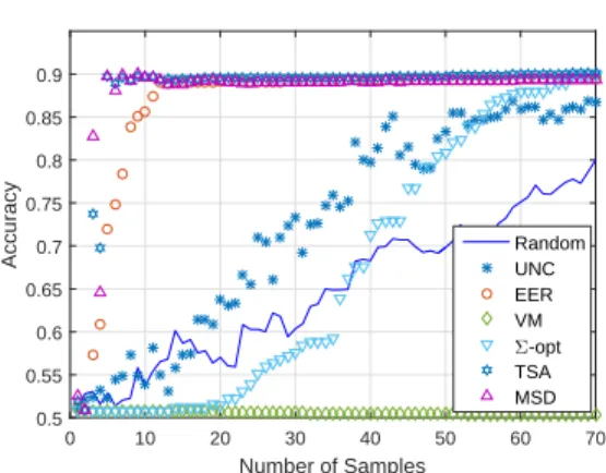
It is worth mentioning that our TV- and MSD-based methods relate to theΣ− optimality-based active learning [89] and the variance minimization [62] correspondingly. This becomes apparent upon recalling thatΣ−optimality and variance-minimization utility score functions are respectively given by UΣ−opt(vi) = kgik21 gii and UV M(vi) := kgik22 gii . Then, further inspection reveals that the metrics are related by

UT V(vi)∝ 1 gii (1−µ2_i)UΣ−opt(vi) (2.30) and correspondingly UMSD(vi)∝ 1 gii (1−µ2_i)UV M(vi). (2.31)

In fact,UT V andUMSD may be interpreted asdata-drivenversions ofUΣ−optandUV M that are enhanced with the uncertainty termg_ii−1(1−µ_i2). On the one hand,UΣ−optandUV M are design-of-experiments-type methods that rely on ensemble criteria and offerofflinesampling schemes more suitable for applications where the setLof nodes mayonlybe labeled as abatch. On the other hand,UT V andUMSD are data-adaptive sampling schemes that adjust to thespecific

realizationof labels, and are expected to outperform their batch counterparts in general. This connection is established due toUV M(vi)andUΣ−opt(vi)beingl2andl1ensembleloss metrics on the GMRF (see equations 2.3 and 2.5 in [12]); similarly, MSD (mean square deviation) and

(40)

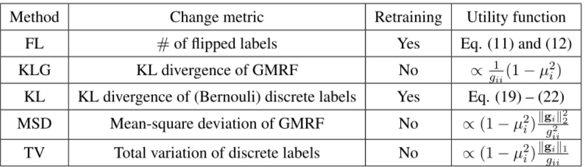
Table 2.1: Summary of EC methods based on different metrics of change

Method Change metric Retraining Utility function

FL #of flipped labels Yes Eq. (11) and (12)

KLG KL divergence of GMRF No ∝ _g1

ii(1−µ

2

i) KL KL divergence of (Bernouli) discrete labels Yes Eq. (19) – (22) MSD Mean-square deviation of GMRF No ∝(1−µ2_i)kgik22

g2

ii

TV Total variation of discrete labels No ∝(1−µ2_i)kgik1 gii

TV (total variation) are alsol2 (on the GMRF distribution) andl1 (on the binary labels pmf) metrics ofchange.

Note that, while the proposed methods were developed for binary classification, they can easily be modified to cope with multiple classes using the one-vs-the-rest trick. Specifically, for any setCof possible classes, it suffices to solve|C|binary problems, each one focused on detecting the presence or absence of a class. Consequently, the maximum among the GMRF meansµ(_ic) ∀c ∈ Creveals which class is the most likely for thei−th node. In addition, the marginal posteriors are readily given by normalizing the binary posteriors in (2.6), that is

p(yi =c) = ¯µ(ic) = µ(_ic)+ 1 P c∈C(µ (c) i + 1) .

Using this approximation, the TV-based scheme can be generalized to

UT V(vi,L)∝ X c∈C h 1−(¯µ(_ic))2ikgik1 gii (2.32)

and similarly for the MSD-based scheme.

A summary of the five different methods that were considered in the context of the proposed EC-based active learning framework is given in Table I.

2.1.4 Computational Complexity analysis

The present section analyzes the computational complexity of implementing the proposed adaptive sampling methods, as well as that of other common adaptive and non-adaptive active learning approaches on graphs. Complexity here refers to float-point multiplications and is given

(41)

Table 2.2: Computational and memory complexity of various methods

Offline Sampling Update Memory

Random O(|E||C|) ∗ ∗ O(|E|+N|C|)

VM [62],Σ-opt [89] O(|L|N2) ∗ ∗ O(N2)

Uncertainty (min. margin) ∗ O(log|C|N) O(|E||C|) O(|E|+N|C|) EER [140], TSA [65] O(|E|N) O(|C|2_N2₎ _O_(N2₎ _O_(N2₎

FL O(|E|N) O(|C|N2) O(N2) O(N2)

TV, MSD O(|E|N) O(|C|N) O(N2) O(N2)

inO(·)notation as function of the number of nodesN, number of edges|E|and number of classes|C|. Three types of computational tasks are considered separately: computations that can be performed offline (e.g., initialization), computations required to update model after a new node is observed (only for adaptive methods), and the complexity of selecting a new node to sample (cf. eq. (2.8)).

Let as begin with the “plain-vanilla” label propagation scenario where nodes are randomly (or passively) sampled. In that case, the online framework described in Algorithm 1 and Section II.B is not necessary and the nodes can be classified offline after collecting|L| samples and obtaining (2.5) for each class inC. Exploiting the sparsity of theL, (2.5) can be approximated via a Power-like iteration (see, e.g., [128]) withO(|E||C|)complexity. Similarly to passive sampling, non-adaptive approaches such as the variance-minimization (VM) in [62] and Σ-opt design in [89] can also be implemented offline. However, unlike passive sampling, the non-adaptive sampling methods require computation ofG0 = (L+δI)−1, which can be approximated with

O(|E|N) multiplications via the Jacobi method. The offline complexity of VM and Σ-opt is dominated by the complexity required to design the label set Lwhich is equivalent to|L|

iterations of Algorithm 1 usingUV M(vi)andUΣ−opt(vi)correspondingly. Thus, the total offline complexity of VM and Σ-opt is O(|L|N2), while O(N2) memory is required to store and processG0.

In the context of adaptive methods, computational efficiency largely depends on whether matrixGis used for sampling and updating. Simple methods such as uncertainty sampling based on minimum margin do not requireGand have soft labels updated after each new sample using

(42)

iterative label-propagation (see, e.g., [86]) withO(|E||C|)complexity. Uncertainty-sampling-based criteria are also typically very lightweight requiring for instance sorting class-wise the soft labels of each node (O(log|C|N)per sample). While uncertainty-based methods are faster and more scalable, their accuracy is typically significantly lower than that of more sophisticated methods that useG. Methods that useGsuch as the proposed EC algorithms in Section III, the expected-error minimization (EER) in [141], and the two-step approximation (TSA) algorithm in [65] all requireO(N2)to perform the update in (2.10). However, TSA and EER use retraining (cf. Remark 3) that incurs complexityO(|C|2_N2₎_{to perform one sample selection; computing the} “expected error” requires fictitiously labeling every unlabeled node, and re-computing the metric by treating the fictitious label as the true label. More specifically, consider the normalization of the binary posteriors that is required (similar to the one discussed in Remark 4) in order to define a posterior pmf over multiple classes (|C|>2). Normalization entails|C|divisions, and happens

|C|times (once for every possible label of an unlabeled node). This gives rise to a nested loop where the outer loop repeats|C|times and the inner loop requires|C|N computations, yielding a total complexityO(|C|2_N)_{for computing the expected error score for one node. Since these} scores have to be computed over all unlabeled nodes (in order to select the best one), the overall complexity to obtain a sample according to EER or TSA isO(|C|2_N2_{). In contrast, the proposed} MSD and TV methods (cf. (2.24), (2.27)) only requireO(|C|N)for sampling. Note that the performance gap between EER and TSA on the one hand, and TV and MSD on the other grows as the number of classes|C|increases.

The complexity analysis is summarized in Table II and indicates that the proposed retraining-free adaptive methods exhibit lower overall complexity than EER and TSA. An important modification is proposed in the ensuing section in order to deal with the challenge ofbiasthat is inherent to all data-adaptive sampling schemes.

2.2

Promoting exploration by adjusting model confidence

It has been observed that active learning schemes may become ”myopic” [113], meaning that they become overly focus onexploiting(focusing on) a small region of the sample space, and neglectexploration. Uncertainty sampling in particular can be prone to such behavior, due to the fact that it is more “myopic,” in the sense that it does not take into account the effect of a potential sample on the generalization capabilities of the classifier. Since the TV- and MSD-based

(43)

Figure