Temi di discussione
(Working papers)
b
er
2
00
8
697
rTechnological change and the demand for currency:
an analysis with household data
The purpose of the Temi di discussione series is to promote the circulation of working papers prepared within the Bank of Italy or presented in Bank seminars by outside economists with the aim of stimulating comments and suggestions.
The views expressed in the articles are those of the authors and do not involve the responsibility of the Bank.
Editorial Board: Patrizio Pagano, Alfonso Rosolia, Ugo Albertazzi, Claudia Biancotti, Giulio Nicoletti, Paolo Pinotti, Enrico Sette, Marco Taboga, Pietro Tommasino, Fabrizio Venditti.
TECHNOLOGICAL CHANGE AND THE DEMAND FOR CURRENCY: AN ANALYSIS WITH HOUSEHOLD DATA
by Francesco Lippi* and Alessandro Secchi** Abstract
Advances in transaction technology allow agents to economize on the cost of cash management. We argue that accounting for the impact of new transaction technologies on currency holding behaviour is important to obtain theoretically consistent estimates of the demand for money. We modify a standard inventory model to study the effect of withdrawal technology on the demand for currency. An empirical specification for households’ demand schedule is suggested, in which both the level of currency holdings and the interest rate elasticity of demand depend on the withdrawal technology available to agents (e.g. ATM card ownership or a high/low density of bank branches, ATMs). The theoretical implications are tested using a unique panel of Italian household data (on currency holdings, deposit interest rates, consumption, development of banking services, etc.) for the period 1989-2004.
JEL Classification: E5.
Keywords: money demand, inventory models, technological change.
Contents
1. Introduction... 3
2. Revisiting previous evidence ... 5
3. A theoretical framework ... 11
3.1 Example 1: Baumol-Tobin with free withdrawals ... 13
3.2 Example 2: A random matching model ... 15
4. Estimation results... 16
5. Discussion and related literature... 21
6. Time series evidence from the 20th century ... 23
7. Concluding remarks... 25
Appendix A: Currency and financial development: the data ... 27
Appendix B: Additional evidence ... 29
References ... 32
_______________________________________
* University of Sassari, EIEF and CEPR. Email: [email protected]
1
Introduction
∗A quantitative assessment of the parameters of the money demand function is im-portant for answering key questions in macroeconomics. Information on the interest elasticity of money demand is helpful in evaluating the distortion induced by infla-tion upon the holdings of non-interest bearing assets, a centerpiece in the analysis of the welfare costs of inflation (e.g. Bailey, 1956; Lucas, 2000). The income elas-ticity is crucial in establishing the money growth rate consistent with price stability (Friedman, 1969).
Yet the wide range of empirical results available in the literature may foster skep-ticism about the stability of money demand and the possibility to provide conclusive answers to those fundamental questions. It is often conjectured that volatile esti-mates of the parameters of money demand may be due to compositional changes in expenditures and the evolution of financial practices. For instance, Teles and Zhou (2005) show that banking deregulation in the United States blurred the traditional distinction between monetary aggregates (e.g. M1 and M2) since it allowed previ-ously illiquid savings accounts to be used for settling transactions. Some of these institutional complications can be avoided by focusing on currency, whose definition is less controversial. Even currency, however, is affected by advances in payment and withdrawal technologies, e.g. by the diffusion of bank branches, electronic points of sale and the ATM network. Such developments confound the linkage between currency, consumption and interest rates, further challenging the identification of the money demand schedule.
We contribute to this debate by presenting a model that accounts for the effect
∗We thank Fernando Alvarez, Giuseppe Bertola, Christian Haefke, Luigi Guiso, Tullio Jappelli,
Tom Sargent and Pedro Teles for helpful discussions. We also benefited from the comments of two anonymous referees and of seminar participants at the Banca d’Italia, the Bank of Portugal, the SED 2005 Budapest Meeting, the European University Institute, the University of Turin, Rome II “Tor Vergata”, LUISS and the 2005 Vienna Macro Workshop. The views are personal and do not involve the responsibility of the institutions with which we are affiliated.
of developments in the withdrawal technology on the demand for currency. To this end, we modify a standard inventory model by introducing a role for the diffusion of bank branches and ATMs withdrawal points on agents’ cash holding choices. The key difference with respect to the classic Baumol - Tobin framework, where all withdrawals are assumed to be costly, is that in our setup agents are occasionally given the opportunity to withdraw at basically no costs, for example when they meet an ATM terminal during a shopping trip. We show that in such an economy both the level and the interest elasticity of the demand for currency decrease as the number of withdrawal opportunities increases. Our dataset shows that the density of bank branches and ATM terminals has a large cross-sectional and time-series dispersion. Thus, accounting for the type of withdrawal technology that is accessible to the households in different regions or periods is potentially important in the estimation of the demand for currency.
The theoretical framework suggests a modified empirical specification of the de-mand for currency, namely one that augments the standard specification with an index of the withdrawal technology and its interaction with the interest rate. We test this specification on a panel of Italian household data over 1989-2004, a period characterized by a widespread heterogeneity in the diffusion of bank branches and ATM terminals. The database includes information on household currency holdings, interest rates on deposit and consumption paid in cash. It also includes information on the households’ access to banking services and the diffusion of the bank branch and ATM networks. An important feature of our investigation is that the data on money holdings, interest rates and expenditures are close counterparts to their theoretical notions. In particular, we use consumption paid with cash as the scale variable for the money demand. This is important because it allows us to isolate the inventory problem (how to finance a given stream of cash consumption expenditure) from the choice of the proportion of total expenditures to be financed in cash. The
latter is influenced by developments in other transaction technologies, such as credit cards or points of sale, which transcend the scope of this paper.
The paper is organized as follows. The next section revisits the money demand estimates of Attanasio, Guiso and Jappelli (2002) using a dataset that almost dou-bles their sample size. The estimation shows that the interest elasticity of money demand changes significantly compared to their results. Section 3 discusses a mod-ification of the inventory model that is used in Section 4 to revisit the household demand for currency. Section 5 discusses the results and offers some comments on related literature. Section 6 presents some evidence on the money demand effects of changes in the banking structure using an aggregate Italian time-series that covers most of the 20th century. A final section summarizes our findings.
2
Revisiting previous evidence
We begin our analysis by replicating the estimation exercise of Attanasio, Guiso and Jappelli (2002) (AGJ henceforth) over a sample that is about twice as large than the one they used. The data, as in their case, are taken from the Survey of Household Income and Wealth (SHIW), an investigation of the economic behaviour of about 8,000 Italian households that is run every two years by the Bank of Italy (see Appendix A). AGJ use four surveys, covering the 1989-1995 period. We benefit from the following four ones, about the 1998-2004 period.
A key premise of the estimation method followed by AGJ is that there are signif-icant differences in households’ access to deposit accounts and withdrawal technolo-gies. In particular, households differ in whether they own a deposit account (the relevant margin for the currency to deposit substitution) and in whether they possess an ATM card (a feature that is likely to affect the marginal cost of withdrawals).1
1Updated summary statistics on Italian households’ money holding behaviour and access to
They argue that heterogeneity in the access to these banking services is likely to be endogenous, affected by factors that also influence money holding behaviour. This instance of endogenous sample selection may give rise to inconsistent estimates of the money demand coefficients if the shocks that affect the household decision to open a bank account or to have an ATM card are correlated to the shocks of the demand for currency. Based on this premise, AGJ estimate a currency demand equation controlling for sample endogeneity by means of Heckman’s (1979) two step methodology.2 The baseline specification for the currency demand equation, derived
from McCallum and Goodfriend’s (1987) extension of the Baumol-Tobin inventory model (see their Section 3), is the following:
logmi,t =
1
1 +β logβ+
1
1 +β logwi,tAi,t−
1
1 +βlogRi,t+ β+γ
1 +β logci,t (1)
wheremdenotes deflated currency holdings,β andw Aare parameters of the trans-action technology,Ris the nominal interest rate andcmeasures the real consumption expenditure.
Our updated replication of AGJ estimates over a much larger sample is pre-sented in Table 1. For ease of comparison, we use the same specification and the same variables they selected. In particular, the equation includes a measure of the interest rate paid on the household deposit account that is disaggregated by year and province,3 the value of nondurable consumption (measured at household level from
SHIW), a linear and a quadratic trend that are intended to proxy for technological progress (the termwi,t Ai,t in equation (1)) and several demographic controls.
2In this particular case Heckman methodology implies the estimation of two probits. First, a
probit for having a bank account is estimated on all the observations. Then a probit for having an ATM card, conditional on having a bank account, is estimated. This allows them to obtain the two variables (Mills’ ratios) that are necessary to correct OLS estimates of the currency demand equation (see AGJ Section 4 for details).
3In Italy there are around 100 provinces. A province is comparable to a U.S. county. Descriptive
statistics on the historical evolution of the mean and the dispersion of interest rates on deposits are available in Appendix A, Table 6.
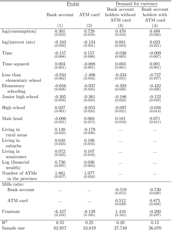
Table 1: Demand for Currency: 1989-2004. Heckman’s two step methodology.
Probit Demand for currency Bank account Bank account Bank account ATM card holders without holders with
ATM card ATM card
(1) (2) (3) (4) log(consumption) 0.301 0.729 0.470 0.488 (0.023) (0.016) (0.016) (0.020) log(interest rate) -0.163 -0.134 0.081 0.023 (0.050) (0.031) (0.024) (0.021) Time -0.157 0.157 -0.036 -0.009 (0.008) (0.006) (0.005) (0.007) Time squared 0.003 -0.008 0.003 0.001 (0.001) (0.001) (0.001) (0.001) Less than -0.834 -1.406 -0.333 -0.727 elementary school (0.062) (0.042) (0.031) (0.057) Elementary -0.656 -0.937 -0.328 -0.422 schooling (0.058) (0.025) (0.026) (0.026) Junior high school -0.305 -0.361 -0.186 -0.122
(0.059) (0.024) (0.022) (0.016) High school 0.027 -0.055 -0.097 -0.056 (0.061) (0.024) (0.021) (0.014) Male head -0.006 0.068 0.101 0.071 (0.021) (0.015) (0.010) (0.011) Living in 0.138 -0.179 ... ... rural areas (0.043) (0.030) Living in 0.048 0.106 ... ... suburbs (0.023) (0.016) Living in 0.072 0.107 ... ... semicenter (0.025) (0.016) Log (financial 0.730 0.036 ... ... wealth) (0.007) (0.004) Number of ATMs 1.861 1.077 ... ... in the province (0.057) (0.034) Mills ratio: Bank account ... ... -0.519 -0.730 (0.015) (0.028) ATM card ... ... 0.512 0.875 (0.029) (0.038) Constant -6.427 -8.129 1.416 -0.200 (0.244) (0.165) (0.161) (0.237) R2 0.55 0.25 0.20 0.15 Sample size 62,957 53,819 27,749 26,070
Note: Standard errors in parenthesis.- The equations are estimated using Heckman’s two-step procedure. The dependent variable in the probit regression for the ownership of a bank account (ATM card) equals one if the household has at least one account (ATM card), zero otherwise. The regressions also include the number of children, number of adults, age, age squared number of income recipients and dummies for employed, self employed and retired heads.
The first stage probits, respectively for the deposit account and the ATM card adoption, are reported in columns (1) and (2) of Table 1. The estimated coefficients show that higher levels of consumption, financial wealth, educational records and ATM withdrawal points increase the probability of adoption of both a bank account and an ATM card. The estimated parameters do not substantially differ from those obtained by restricting the sample to 1995, with the only exception of the negative effect of the (log) interest rate on the adoption of both.
The currency demand estimates concern households who possess a deposit ac-count. Two separate demand equations are estimated, one for the households with-out an ATM card and one for those who possess an ATM card. The estimates are shown in columns (3) and (4) of Table 1, respectively. These indicate values for the coefficients of consumption and the demographic variables which are broadly in line with the ones of AGJ. The point estimate of the consumption elasticity is close to 0.5, the value predicted by the classical Baumol - Tobin model.
Different results from the ones of AGJ emerge instead for what concerns the estimated interest rate elasticity. Column (3) shows a positive (statistically signifi-cant) elasticity for the households without ATM card, which compares to a negative (statistically significant) value of -0.27 found by AGJ. For the households with ATM card, column (4) reports an interest elasticity that is not statistically different from zero. This compares to a point estimate of -0.59 found by AGJ over the 1989-1995 sample.
The positive (albeit small) interest rate coefficients that appear in the full sample estimates, and the large differences between those and AGJ estimates, suggest a misspecification problem.4 Three possible sources of misspecification are considered
next. First, the linear quadratic trend used to proxy for technological progress in the withdrawal technology may impose too much of a structure over a long time
period.5 Second, the sizable heterogeneity of the micro data (witnessed by the low
values of the fit statistics) signals the presence of other unobserved factors affecting money demand. Systematic year or regional distribution of these factors, as is likely the case for the level of petty crime or the diffusion of economic activities that rely on cash (e.g. street markets, the black economy), may give rise to an omitted variable problem. Based on these considerations, the regressions presented below use year and province dummies to remove unobserved time and regional factors affecting currency demand.6 Third, the functional form of the demand for currency
rather than obeying a constant interest rate elasticity (as implied by the log-log specification in (1)) may feature a different functional form, such as constant semi-elasticity (log-lin).
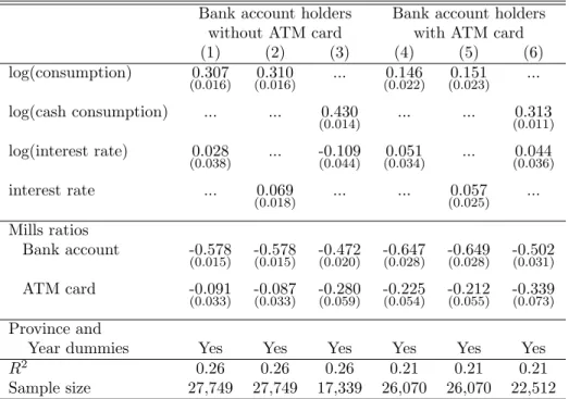
These issues are tackled by the regressions presented in Table 2. In the first set, shown in columns (1) and (4), the trend and its square are replaced by year and province dummies. The estimation results show that this specification deliv-ers a near zero interest elasticity for both types of households, although the point estimates of the interest rate coefficient remain positive. Note, moreover, that the consumption coefficients for both types of households become much smaller (we discuss the properties of the scale variable below).
In the regressions of columns (2) and (5) the logarithm of the interest rate is replaced by the level, thus stipulating that the elasticity varies with the interest rate. This modification does not solve the puzzling finding of a positive interest elasticity. Additional experiments with alternative functional forms, including poly-nomial specification as well as Box-Cox transformations, do not deliver any sensible improvement in the fit of the model or the sign of the interest rate elasticity (not reported in the table).
5Note that in a sample that includes four periods, a linear and a quadratic trend work “almost”
like time dummies.
6A robustness exercise discussed in Section 4 estimates the currency demand equation by
Table 2: Demand for Currency: Alternative specifications.
Bank account holders Bank account holders without ATM card with ATM card (1) (2) (3) (4) (5) (6) log(consumption) 0.307 0.310 ... 0.146 0.151 ... (0.016) (0.016) (0.022) (0.023) log(cash consumption) ... ... 0.430 ... ... 0.313 (0.014) (0.011) log(interest rate) 0.028 ... -0.109 0.051 ... 0.044 (0.038) (0.044) (0.034) (0.036) interest rate ... 0.069 ... ... 0.057 ... (0.018) (0.025) Mills ratios Bank account -0.578 -0.578 -0.472 -0.647 -0.649 -0.502 (0.015) (0.015) (0.020) (0.028) (0.028) (0.031) ATM card -0.091 -0.087 -0.280 -0.225 -0.212 -0.339 (0.033) (0.033) (0.059) (0.054) (0.055) (0.073) Province and
Year dummies Yes Yes Yes Yes Yes Yes
R2 0.26 0.26 0.26 0.21 0.21 0.21
Sample size 27,749 27,749 17,339 26,070 26,070 22,512 Note: Standard errors in parenthesis. The equations are estimated using Heckman’s two-step procedure. The coefficients of the first stage probit regression are reported in Table 8. The other variables included in the second stage regressions are as in Table 1. Equations (3) and (6) are estimated over the sample period 1993-2004, the remaining equations over the sample 1989-2004.
Lastly, we analyze the role of the scale variable. The measure used above ag-gregates non durable consumption and service purchases irrespective of the way the agents pay for it. The large diffusion of debit and credit cards networks occurred throughout the period is likely to make this variable inappropriate for the estimation of the cash inventory model (the low consumption elasticities detected in (1) and (4) may be a consequence of this). A more appropriate scale variable, the household expenditures done in cash, is available from SHIWsince 1993. The regressions that use the cash consumption variable are presented in columns (3) and (6). The con-sumption coefficients increase substantially, although they remain below one half. A small and negative interest rate elasticity is detected for the households without ATM card (at -0.1); the one for agents with ATM remains small and not significantly
different from zero.7
Altogether, the currency demand regressions presented above yield estimates of the interest rate elasticity that are small and scattered around zero, in the -0.1 to 0.1 range. Our preferred specification, which controls for unobserved time and provincial effects and uses cash consumption as a scale variable (columns 3 and 6 of Table 2), eliminates the puzzling finding of a positive interest rate coefficient. However, the estimated interest elasticities remain small (-0.1 for agents without ATM and zero for the others) compared to previous estimates and to the predictions of inventory models such as Baumol-Tobin or Miller-Orr (which are equal to, respectively, -1/2 and -1/3).8 The rest of this paper investigates the possibility that the developments
in withdrawal technology occurred in Italy over the period considered, namely the strong diffusion of bank branches and the ATM terminals, may contribute to explain the low and unstable interest rate coefficients detected above. To this end, the next section discusses the consequences of such developments for standard inventory models of the demand for currency.
3
A theoretical framework
This section presents a modification to the standard inventory model that investi-gates the relation between the withdrawal technology and the demand for currency. The distinguishing feature of the model is to account for the currency demand effect 7Note, for comparability, that estimates of equations (3) and (6) using non-durable consumption
over the 1993-2004 period yield an interest rate elasticity of -0.05 for households without ATM card, of 0.06 for households with ATM card.
8The possibility of a low interest elasticity at low interest rates is discussed by Mulligan and
Sala-i-Martin (2000). In their model agents must pay a fixed cost to have a deposit account, which is shut down when its return falls below the cost (agents with little savings or low return will close it first). They show that this effect may lower the interest elasticity estimated onaggregate
data. Note however that our households data are not affected by this effect as we only use data for the agents who do possess a deposit account (taking into account the sample selection problem). Moreover, as shown in Appendix A, Table 6, no clear signs of a reduction in the number of agents who possess a deposit account emerge from the data over time.
of the diffusion of cash dispensers (ATM terminals or bank branches). We consider the steady state problem of an agent who uses cash to finance an exogenous stream of consumption expenditure equal toc. Shopping takes place in one of several loca-tions of the economy, which may be endowed with a cash dispenser that allows the agent to withdraw cash without incurring a time cost. By contrast, a withdrawal done at a location without cash dispenser entails a cost b, as in the Baumol-Tobin model, as the agent wastes some resources to walk to the bank.
LetT(M, c) be the number of costly withdrawals from the bank that are neces-sary to finance a consumption flowcwhen the average money balances are M. We assume thatT is decreasing inM, so that higher balances allow the agent to finance consumption with less withdrawals, and thatT is convex inM, so the minimization problem is well behaved. The money demand solves the minimization problem:
min
M R M +b T(M, c) (2)
where R is the net nominal interest rate. The optimal choice of M balances the impact on the cost due to forgone interest with the effect on the cost of withdrawals. To analyze the effect of technological change in T on the money demand we present two comparative static results, one about the level of money demand and the other about its interest rate elasticity. Consider two withdrawal technologiesTi
and the associated money demand schedules, Mi for i = 1,2. Note that the first
order condition of problem (2) and the assumption thatT is convex in M yield:
Result 1. If the marginal cost of withdrawals is higher then the money demand is lower. Formally, ifT0
2(M)≥T10(M) for all M then M2 ≤M1 for all R ≥0.
The second result relates the interest rate elasticity to the curvature of the cost function T. In particular, the first order condition of problem (2) and its total
differential imply: −R M ∂M ∂R = 1 / µ M T00 −T0 ¶ (3) The expression −M T00/T0 ≥ 0 is a measure of the local curvature of the cost
functionT. It is also the elasticity of the marginal cost T0. Thus equation (3) says
that if the marginal cost is more sensitive to M, then the money demand is less sensitive to interest rate changes. This yields:
Result 2. If the interest rate elasticity of the marginal cost of withdrawals is higher, the interest rate elasticity of the money demand is smaller. Formally, assume that at a given R: M2 T 00 2(M2) −T0 2(M2) ≥ M1 T00 1(M1) −T0 1(M1) , then − R M2 ∂M2 ∂R ≤ −MR1 ∂M1 ∂R
where M1 and M2 denote, respectively, the demand for currency implied by
technol-ogyT1 and T2 when the interest rate is R.
We now use these results to analyze the effect of technological progress in T on money demand for two alternative withdrawal technology specifications.
3.1
Example 1: Baumol-Tobin with free withdrawals
We consider a Baumol - Tobin setup and assume that in every period the agent has p contacts with the financial intermediary (opportunities to withdraw) which come for free. Withdrawals in excess of p are costly. To think of an application, imagine an agent who passes by a bank branch once a week on her way to the ball game. This case can be represented by a technologyTp saying that she has one free
withdrawal a week, orp= 1. Now suppose that an ATM is installed on the way to her job and that she works six days per week. This “technological change” can be represented by an increase inp, so that she gets seven free withdrawals a week. The
above setup is described by the following technology:
Tp(M, c) = max{ c
2 M −p,0}. (4)
where Tp denotes the number of costly withdrawals and the parameter p gives the
number of free withdrawals per unit of time.
Setting p= 0 in (4) stipulates that all trips are costly, as in the Baumol-Tobin model:9 T
0(M, c) = 2cM. Note thatT0has a marginal cost functionT00 with constant
elasticity equal to 2, which implies the well known result that the interest elasticity of the money demand is 1/2. The interpretation of the p > 0 case is that the agent has pfree withdrawals, so that if the total number of withdrawals is c/(2 M), then she pays only for the excess ofc/(2M) over p.
The money demand for a technology with p≥0 is given by
Mp(R) = q b c 2 R forR ≥R∗ q b c 2 R∗for R < R∗ (5) where R∗ ≡(p)22b/c . (6)
When p = 0 the forgone interest cost is small at low values of R, so agents economize on costly withdrawals and choose a large value of M. Now consider
p > 0. In this case there is no reason to have less than p withdrawals per unit of time, since these are free. Hence, forR < R∗ agents choose the same level of money
holdings, namely, Mp(R) = Mp(R∗), since they are not paying for any withdrawal
but they are subject to positive forgone interest rate costs.
Note that improvements in the particular technology described in (4) produce 9An agent with consumption flow c withdraws 2 M, which last 2M/c periods, has average
a money demand that is lower in level and has a smaller interest rate elasticity (in between zero and one-half) because it indeed satisfies the assumptions for results 1 and 2 presented above. To see this, consider two technologies indexed by 0≤p1 < p2.
These technologies satisfy the following three properties:
(i) A greater value ofprepresents technological progress, becauseTpis decreasing
inp. FormallyTp2(M, c)≤Tp1(M, c) (with strict inequality forM < c/(2p1)).
(ii) a higher value of p increases the marginal cost T0
p, hence decreases money
demand by result 1, at least for some values of M. In particular, 0 =T0
p2(M, c) > T0
p1(M, c) over the range: c/(2p2)< M < c/(2 p1), and equal otherwise.
(iii) A greater value ofpincreases the curvature ofTp, hence decreases the
inter-est elasticity by result 2. To see this notice thatTp2 can be obtained by the following
transformationTp2(M, c) =g(Tp1(M, c)) for g(τ) = max{τ−(p2−p1),0}. As the
transformation is increasing and convex inτ, it follows that technologies indexed by a higher value ofp have more curvature.
3.2
Example 2: A random matching model
This section studies the effect of bank branch (ATM terminals) diffusion on currency demand using a random matching framework. We consider an economy with two locations: the shopping center and the financial district. The agent incurs a time cost b whenever she visits the financial district to withdraw money. Let c be the agent daily consumption andp ∈(0,1) be the probability that the agent is offered an opportunity to withdraw for free in the shopping center (e.g. from an ATM). Note that a withdrawal of 2M allows her to finance at least 2M/c consecutive days in the shopping center (i.e. without having to go to the financial district). The probability that the agent is not matched with a cash dispenser during this period is (1−p)2Mc , that for small p can be approximated by e−2M pc . This probability
gives the fraction of total trips ( c
transaction technology:
Tp(M, c) = c
2Me
−2M pc (7)
whereTp denotes the average number of costly withdrawals for an agent who
with-draws 2M and consumes c.10
As for the case discussed in Section 3.1 it is immediate to show that the tech-nology in (7) has the following features: (i) Tp is decreasing in p, so that higher
values ofprepresent technological progress; (ii) the marginal costT0
p is increasing in pwhich, by result 1, implies that the level of money demand decreases as the tech-nology improves; (iii) the curvature of the cost function, as measured by ¡M T00
−T0 ¢
, is increasing in p which, by result 2, implies that the interest rate elasticity of the money demand is smaller for better technologies.11
4
Estimation results
The theory discussed in the previous section shows that the level and the interest elasticity of the demand for currency depend on the type of withdrawal technology that is available to agents. In particular, it suggests that technological improve-ments, i.e. reductions in the cost of withdrawals, lower the level of the money demand and its interest elasticity (in absolute value). Based on these insights, we construct a proxy for the level of the withdrawal technology faced by the household 10The use of equation (7) in problem (2) assumes that the ratio between the average withdrawal
and the average balance is equal to 2. This is only an approximation, as the exact computation must take into account that the money holding profile is not saw-tooth, and that with random matches some withdrawals occur before a zero balance is reached. See Alvarez and Lippi (2006) for such an extension.
11Some algebra shows that ³M T00
−T0
´
= 2 + c(2(2pMpM+)2c) which is increasing in p. Result (iii) is alternatively established by noting that, given p2 > p1, Tp2 can be obtained by applying the
following increasing and convex transformation toTp1:
g(τ) = (τ)2 c
and estimate a specification of the demand for currency that includes this variable both in level and interacted with the interest rate.
We proxy for the level of the withdrawal technology faced by agents by using the number of bank branches per capita measured at city level (around 300 cities per year). This indicator, whose year averages and standard deviations are reported in Table 7 of Appendix A, highlights the ongoing diffusion of bank services across the territory over the past fifteen years as well as its large cross section dispersions.12
To make the results comparable with those described in Section 2 the currency demand estimates presented in the next Table use the same set of regressors of Table 2. All regressions feature cash-expenditure rather than non-durable consumption as a scale variable, and use year and province dummies in the place of the linear-quadratic trend.13
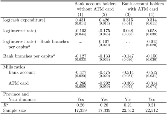
Our first set of results, that controls for endogeneity in the access to bank services, is presented in Table 3. The Heckman second step regressions reported in columns (1) and (2) concern agents without ATM card. This is the group for which our measure of withdrawal technology - the number of bank branches per capita at the city level - is most appropriate.
The specification in column (1) integrates the technology measure in level. In line with the predictions of the theory, a greater diffusion of bank branches reduces currency holdings and the interest rate enters the equation with a negative and statistically significant coefficient.
Column (2) considers a specification which allows the technology index to affect both the level and the interest elasticity of the demand for currency, as the theory 12Until the early nineties commercial banks faced restrictions to open new bank branches in other
provinces. A gradual process of liberalization has occurred since then, which has led to a sharp increase in the number of bank branches and a reduction of the interest rate differentials across different areas (see Casolaro, Gambacorta and Guiso (2006) for a review of the main developments in the banking industry during the past two decades).
13None of these choices is really key for the results that follow. Qualitatively similar estimates
Table 3: The Demand for Currency and Withdrawal Technology
Bank account holders Bank account holders without ATM card with ATM card
(1) (2) (3) (4)
log(cash expenditure) 0.431 0.426 0.315 0.314
(0.014) (0.014) (0.011) (0.011)
log(interest rate) -0.103 -0.175 0.048 0.058
(0.044) (0.046) (0.036) (0.038)
log(interest rate)·Bank branches ... 0.107 ... -0.015
per capitaa (0.020) (0.020)
Bank branches per capitaa -0.127 -0.133 -0.147 -0.150
(0.033) (0.033) (0.030) (0.030) Mills ratios Bank account -0.477 -0.475 -0.514 -0.512 (0.020) (0.020) (0.031) (0.031) ATM card -0.266 -0.292 -0.305 -0.314 (0.059) (0.059) (0.073) (0.074) Province and
Year dummies Yes Yes Yes Yes
R2 0.26 0.26 0.21 0.21
Sample size 17,339 17,339 22,512 22,512 Note: Standard errors in parenthesis. The equations are estimated using Heckman’s two-step procedure. The coefficients of the first stage probit regression are reported in Table 9. The other variables included in the second stage regressions are as in Table 1.
a Number of bank branches per capita measured at the city level.
predicts. The estimates confirm the findings of column (1) that a greater diffusion of bank branches reduces currency holdings and that the interest rate (log) level en-ters the equation with a negative coefficient. Moreover, the interaction between the interest rate and the diffusion term enters significantly with a positive coefficient. This suggests that the interest elasticity of the demand for currency varies across households, with lower values for households who face more a superior technology (a greater diffusion of bank branches). The comparison of (1) and (2) shows that omitting the interaction term from the estimation yields an estimate of the average
interest rate elasticity that neglects an important layer of heterogeneity. In quanti-tative terms, the estimates imply that agents faced with less developed technology, e.g. a diffusion value of 0.1 (the 5th percentile), have an interest elasticity of about
diffusion indicator is around 0.5) and is basically nil for the households facing the highest levels of development.
The regressions in columns (3) and (4) concern households who possess an ATM card. We attempt this estimation exercise even though we are aware of the fact that our index for the development of the withdrawal technology - the diffusion of bank branches per capita at the city level - is not the most appropriate measure of diffusion for this type of household.14 The estimation results should thus be taken
with a grain of salt, as they may be subject to a greater amount of measurement error than the ones concerning the households without ATM.
In both regressions the level of currency holdings is negatively related to the diffusion of bank branches, with a coefficient magnitude comparable to the one detected for the agents without ATM card. Instead, the interest rate coefficients (both levels and interactions) are not significantly different from zero. In principle, a zero interest elasticity for agents who face a more advanced withdrawal technology can be explained by the models outlined in Section 3. For instance, the Baumol-Tobin model with free withdrawals predicts that the interest rate range over which the demand for currency has a zero interest elasticity expands with technological advances.
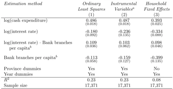
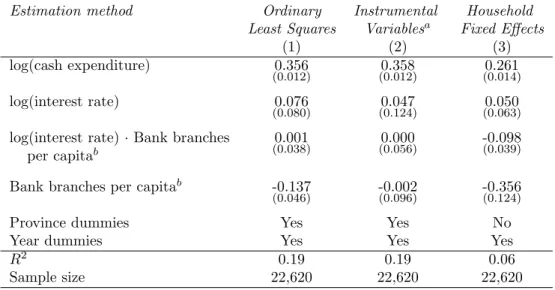
We conclude this section by exploring the robustness of the estimates. The results for the households without ATM card are shown in Table 4.15 For all regressions,
we compute the coefficients’ standard errors by accounting for the possibility of heteroschedasticity and cross correlation of the shocks within a province in a given year.16 We begin by assessing whether the estimated coefficients were affected by
14Unfortunately information on the diffusion of ATM terminals, the natural diffusion measure
for the ATM card holders, is not available to us at the city level but only at the province level (about 100 datapoint per cross section).
15The corresponding results for the households with ATM card are reported in Appendix C
(Table 10).
16The standard errors presented in Tables 2 and 3 do not control for heteroschedasticity and
the choice of the Heckman estimation method. The identification of the currency demand coefficients in the presence of sample endogeneity hinges on the specification of the probit selection equation. In particular, if the first and the second stage OLS have a large set of variables in common, a collinearity problem may occur as the Mills ratio is approximately a linear function of these variables over a wide range of values (see Puhani, 2000).17 To assess the impact of multicollinearity on the
baseline results of column (2) of Table 3 we present a plain OLS estimate of the demand for currency in column (1) of Table 4. The results show that coefficients on cash consumption and the interest rate are similar to those estimated in Table 3.
Table 4: The Demand for Currency and Withdrawal Technology: Robustness.
Bank account holders without ATM card
Estimation method Ordinary Instrumental Household
Least Squares Variablesa Fixed Effects
(1) (2) (3)
log(cash expenditure) 0.486 0.487 0.393
(0.018) (0.018) (0.025)
log(interest rate) -0.180 -0.236 -0.334
(0.092) (0.135) (0.088)
log(interest rate)·Bank branches 0.109 0.103 0.098 per capitab (0.036) (0.062) (0.046)
Bank branches per capitab -0.113 -0.159 -0.399
(0.058) (0.127) (0.135)
Province dummies Yes Yes No
Year dummies Yes Yes Yes
R2 0.23 0.23 0.08
Sample size 17,371 17,371 17,371
Note: Robust standard errors in parenthesis. The other regressors are as in Table 1. -aThe instruments used for the deposit interest rate and the number of bank branches
at the city level are the interest rate lagged value and the number of firms and employ-ees per resident at the city level. -b Number of bank branches per capita measured
at the city level.
We consider next the possibility that some of the regressors are not exogenous 17The Montecarlo evidence surveyed in Puhani (2000) shows that, based on standard
evalu-ation criteria, OLS is often superior to limited informevalu-ation maximum likelihood in the case of multicollinearity. In our case a suspect multicollinearity problem is signalled by the fact that the regression of the Mills ratio of the ATM adoption on the other regressors of the second stage OLS yields anR2statistic of 95 per cent.
with respect to the currency demand shocks. This issue might arise both for the number of bank branches per city and the deposit interest rate at the province level, which might move in response to currency demand shocks that are common to all households of a given city or province. To this end we study the sensitivity of the results in Table 3 instrumenting the interest rates with the previous-year value and the number of bank branches with the number of firms in the area. The results, reported in column (2) of Table 4, do not show significant differences with respect to the benchmark estimates of Table 3.18
Finally, column (3) of Table 4 presents results obtained by a fixed effect estimate, which controls for household-specific unobserved factors. The estimated coefficients of the consumption, interest rate and bank branch diffusion are statistically signif-icant and maintain the expected sign. The point estimates of the direct (negative) effect of bank branch diffusion on currency holdings and the average interest elas-ticity (about -0.3) are somewhat larger than the values reported in columns (1) and (2). The coefficient of the interaction term is unaffected, confirming the pre-vious estimate of the marginal effect of technological advances on the interest rate elasticity.
5
Discussion and related literature
The evidence on the households money demand discussed in the previous section is consistent with the theory presented in Section 3, which predicts that the level and interest elasticity of money demand decrease with developments in the withdrawal technology.
Other studies, based on cross-section or time series data, have analyzed the effects 18The fact that the estimates obtained through OLS and IV are very similar provides evidence
in support of a limited relevance of endogeneity problems, an hypothesis confirmed by standard exogeneity tests on the three variables (not reported).
of financial innovation on the level of the money demand. Duca and Whitesell (1995), who follow a cross-sectional approach based on US household survey data, find that credit card ownership is associated with lower money holdings. AGJ highlight, based on Italian survey data, that ATM users hold significantly lower cash balances than non-users. Similarly, Stix (2004) offers evidence concerning Austrian individuals showing that the demand for purse cash is significantly smaller for ATM users. Overall, the evidence consistently indicates that innovations in withdrawal (ATM cards) and payment instruments (credit cards) reduce the level of money balances that agents hold.
Concerning the interest elasticity of the demand for currency, our estimates in-dicate a value in the -0.3 to -0.1 range for the median household without ATM card. A basically zero elasticity is found for agents with an ATM card. These values are within the range of theoretically plausible elasticities predicted by the models of Section 3.
The estimated interest elasticity for the households without ATM is close to the one detected by AGJ, which is -0.27. A stark difference emerges instead for the households with ATM card, whose interest elasticity was estimated at -0.59 based on the 1989-1995 surveys, but turns out to be essentially nil using the full sample period. In our view the latter finding is to be preferred to the high elasticity found over the smaller sample, not just because of the greater amount of information upon which it is based but also because it is consistent with the theoretical prediction that agents with more developed withdrawal technologies (e.g. ATM card holders) are expected to have a smaller interest elasticity.19
The findings concerning the elasticity with respect to the scale variable (non-19This proposition, which holds true for the models discussed in Section 3, is also consistent with
the McCallum-Goodfriend model that underlies AGJ formulation. That model can be written in terms of problem (2) by defining the transaction technology: T(M, c) =Acγ¡c
M ¢β
whereA,βand
γ are technological parameters and c denotes consumption. A smaller interest elasticity requires a larger value of the parameterβ. A greater value of this parameter corresponds to technological development as it reduces the cost of withdrawals providedc/M <1.
durable consumption or cash-expenditure) that emerge from the various specifica-tions indicate values that are close, sometimes a little below, one-half. These esti-mates, which are essentially based upon the cross-sectional variation (due to our use of year dummies), differ from the near-unit elasticity that emerges by the analyses of long time-series, e.g. Lucas (1988, 2000) and Meltzer (1963), and is predicted by many theoretical models. The issue is of interest in the debate on the optimality of the Friedman rule (e.g. De Fiore and Teles, 2003). A simple reconciliation between the long-run unit elasticity of consumption and the smaller values detected over the cross-sectional household data is that the cost of a trip to the bank, b, is linked to the consumption (income) variable in the long-run but less so in the cross-section (or the short-run). It is reasonable to presume that theb cost is related to the wages in the banking sector which, over a long time period, is proportional to aggregate wages and consumption. Formally, assuming a proportionality relation between b
and c yields a unit income elasticity if one maintains the reasonable assumption that the transaction technology T(M, c) in problem (2) is homogenous of degree zero in M and c (as in the example economies discussed in Section 3).20 The next
section presents estimates of the demand for currency in Italy based on a centen-nial time-series (yearly data), from 1890 to 1998 (the last year before the euro was introduced). The unit elasticity is strongly supported by the time-series evidence. The estimated interest elasticity is about -0.3, a value that is consistent with the estimates that were found above.
6
Time series evidence from the
20
thcentury
This section investigates the robustness of the results based on disaggregated data using a long time-series for aggregate Italian data. We estimate a specification of the 20The proof follows immediately from the first order condition of problem (2): −R = b T0(M, c).
demand for currency that accounts for developments in withdrawal technology, as proxied by the diffusion of bank branches. The evidence is based on annual Italian data from 1936 to 1998.21 The results are reported in Table 5.
Table 5: Currency Demand in Italy : 1936-1998.
Dependent variable: log(real currency holdings)
Levels First differences
(1) (2) (3) (4)
log(real GDP) 0.878 1.032 1.065 0.749
(0.058) (0.071) (0.073) (0.141)
log(interest rate) -0.217 -0.283 -0.505 -0.377
(0.075) (0.058) (0.241) (0.188)
log(interest rate)·Bank branches 0.833 0.819
per capita (0.767) (0.500)
Bank branches per capita -1.202 -3.021 -2.944
(0.423) (1.676) (1.769)
Number of observations 63 63 63 62
Newey-West standard errors in parenthesis. - All regressions include a year dummy for the war year 1944.
In column (1) we report the results of the estimation of a baseline money demand equation relating real currency holdings to GDP and the nominal interest rate. The estimates detect a near-unit income elasticity, in line with previous results based on long time-series and theoretical models (see e.g. Lucas, 1988, Lucas, 2000 and Meltzer, 1963). The interest rate elasticity, although significantly below one-half, is comparable to the one found by previous studies. In the regression of column (2) the baseline money demand equation is augmented with a proxy for the development of the withdrawal technology, namely the ratio between the number of bank branches and population. This variable enters the equation significantly and with a negative sign, suggesting that a greater diffusion of bank branches reduces currency holdings, 21The sample size is constrained because data on the number of bank branches are available only
from 1936. The GDP data is from Fenoaltea (2005) and the national statistical institute (ISTAT), the price level from ISTAT, currency in circulation and interest rates from De Mattia (1967), the number of bank branches from Banca d’Italia (1977).
as predicted by the theory. Compared to the estimates of column (1) both the income and the interest rate elasticity increase, although the latter remains below one-half.
In column (3) we present our preferred specification for the currency demand equation, which includes the interaction between the (log) interest rate and bank-branch diffusion. The point estimates suggest an income elasticity not significantly different from one and a lower bound for the interest rate elasticity equal to one-half.22 Moreover, the signs of the financial diffusion variable (both for the level and
the interaction with the interest rate) are in line with the theoretical predictions of Section 3. The point estimates suggest that over seventy years the interest rate elasticity in Italy declined from around -0.4 to -0.1. Note that the interaction term is not statistically different from zero. This is likely due to a multicollinearity problem, as suggested by the high level of the condition number and by the fact that the regression of the interaction term on the interest rate and of financial diffusion yields anR2 above 98 per cent. A tentative assessment of the effects of multicollinearity on
the estimated parameters is provided in column (4) where we present results based on first-differenced variables.23 These estimates confirm sign and magnitude of the
financial diffusion coefficients detected in the level regressions (the p-values for the interaction and level terms of financial diffusion are both equal to ten per cent).
7
Concluding remarks
This paper contributes to the quest for accurate quantitative estimates of the param-eters that govern the money demand function. We argue that accounting for tech-nological development is important to identify theoretically consistent estimates of
22The lower bound is reached for a near zero level of financial diffusion.
23We are aware that first differencing, even if it is often suggested as a remedy for multicollinearity
the demand schedule. We base our analysis on an original household level database that provides us with empirical observations that closely match their theoretical counterpart over the 1989-2004 period.
The analysis is guided by a theoretical framework on the money demand effect that are caused by advances in the withdrawal technology. The main theoretical implication of the model is that technological development has an effect on average money holding and on the interest elasticity of money demand. The latter prediction is the novel implication of this paper. These insights are tested by augmenting a standard money demand equation with a proxy for the technology level faced by households (the number of per capita bank branches) and its interaction with the interest rate.
Our results, which are robust to different estimation methods, suggest that the money demand is significantly affected by advances in the withdrawal technology. In particular, for the households that do not have an ATM card, the density of bank branches and its interaction with the interest rate enter the money demand equation with the sign predicted by the theory. The estimates suggest that the interest elasticity of money demand lies in between 0.2, for households who face the least developed withdrawal technology, and zero, for the ones facing the highest one. The micro evidence upon which our results are based is drawn from the 1993-2004 period. The analysis of an aggregate Italian time-series for a much longer period covering most of the 20th century confirms the impact of financial development on
Appendix
A
Currency and financial development: the data
Our analysis relies on a dataset drawn from the Survey of Household Income and Wealth (SHIW), a periodic survey conducted by the Bank of Italy since 1965 on a rotating sample of Italian households. The survey collects information on several social and economic characteristics of the household members, such as age, gender, education, employment, income, real and financial wealth, consumption and saving behavior. Each survey is conducted on a sample of about 8,000 households. We focus on the surveys conducted from 1989 to 2004 because they include a section dedicated to the household cash management. This contains data on the average amount of cash held by the household and information on the household access to various means of withdrawal and deposit. Annual sample means of some variables related to the household currency management are reported in Table 6.
Table 6: Italian household: currency management
Variable 1989 1991 1993 1995 1998 2000 2002 2004 Fraction with a checking account 0.88 0.86 0.84 0.85 0.85 0.85 0.86 0.86 Fraction using ATMs 0.15 0.29 0.34 0.40 0.49 0.52 0.56 0.58 Average currency holdings 705 581 417 466 407 393 394 400
No bank account 694 609 382 463 395 416 521 550 With bank account 707 577 423 467 409 389 373 376 No ATM card 697 601 448 506 444 448 425 422 With ATM card 754 530 386 423 382 352 345 354 Nondurable consumption 1,644 1,544 1,572 1,632 1,537 1,600 1,633 1,705 Cash consumption ... ... 1,025 1,036 910 923 889 871 Total number of observations 8,274 8,188 8,089 8,135 7,147 8,001 8,011 8,012
Source: Bank of Italy -Survey of Household Income and Wealth. Entries computed using sample weights. Nominal variables are deflated and expressed in euro (base: 2004). -Nondurable and cash consumption are averages per month.
The first line shows that about 15 per cent of the households did not hold a checking account in 2002, a value that is near that recorded in 1989. During the same period, the fraction of households who possess an ATM card increases sharply, from 15 to 55 per cent. Concerning real currency holdings, the average amount held by the household almost halves during the last 15 years. The reduction, which is common across households with different withdrawal technologies, is largest for those who own an ATM card.
Table 7 reports summary statistics on the supply of bank services, such as the diffusion of bank branches, ATM terminals, and on the interest rate paid on de-posits.24 Note that interest rates paid on deposits record a substantial reduction
since 1989, although they maintain a relatively large cross-sectional variation even in more recent years (this is important to estimate the interest elasticity).
Table 7: Financial development and interest rates
Variable 1989 1991 1993 1995 1998 2000 2002 2004 Bank branchesa ... 0.35 0.41 0.44 0.49 0.53 0.54 0.57 (0.19) (0.23) (0.24) (0.24) (0.27) (0.31) (0.31) ATM pointsb 0.10 0.22 0.32 0.39 0.51 0.57 0.65 0.65 (0.07) (0.13) (0.18) (0.19) (0.22) (0.22) (0.23) (0.22) Interest ratec 6.90 6.69 6.07 5.18 2.14 1.13 0.77 0.33 (0.48) (0.52) (0.45) (0.32) (0.22) (0.21) (0.15) (0.12)
Entries computed using sample weights. - Standard deviation in parenthesis. -a Per
thou-sand residents; individual observations disaggregated at city level. bPer thousand residents;
individual observations disaggregated at provincial level. c Individual observations
disag-gregated at provincial level (source: Central credit register).
Central Credit Register (See Miller (2000) for a detailed description of this database). Information is available for each year and province. Italian provinces were 95 until 1995 and became 103 afterwards. The size of a province is broadly comparable to that of a U.S. county).
B
Additional evidence
Table 8: Probit (first stage analysis for Table 2)
Probit for equations (1) and (4) Probit for equations (2) and (5) Probit for equations (3) and (6) Bank account ATM card Bank account ATM card Bank account ATM card log(consumption) 0.301 0.729 0.304 0.727 (0.023) (0.016) (0.024) (0.016) log(cash expenditure) -0.092 0.197 (0.023) (0.013) log(interest rate) -0.163 -0.134 -0.271 0.129 (0.050) (0.031) (0.095) (0.055) interest rate -0.123 0.066 (0.039) (0.031)
Province and Yes Yes Yes Yes Yes Yes
Year dummies
R2 0.55 0.25 0.58 0.27 0.61 0.21
Sample size 62,957 53,819 62,957 53,819 46,756 39,851 Note: The dependent variable in the probit regression for the ownership of a bank account (ATM card) equals one if the household has at least one account (ATM card), zero otherwise. The other regressors are as in Table 1.
Table 9: Probit (first stage analysis for Table 3)
Probit for equations (1) and (3) Probit for equations (2) and (4) Bank account ATM card Bank account ATM card log(cash expenditure) -0.092 0.197 -0.092 0.196
(0.023) (0.013) (0.023) (0.013)
log(interest rate) -0.271 0.129 -0.250 0.019
(0.095) (0.055) (0.110) (0.068)
log(interest rate)·Number -0.057 0.245
of bank branches in the city (0.151) (0.089) Number of bank branches 0.373 0.281 0.364 0.306
in the city (0.238) (0.142) (0.239) (0.142)
Province and Yes Yes Yes Yes
Year dummies
R2 0.61 0.21 0.61 0.21
Sample size 46,756 39,851 46,756 39,851
Note: Standard errors in parenthesis. The dependent variable in the probit regression for the ownership of a bank account (ATM card) equals one if the household has at least one account (ATM card), zero otherwise. The other regressors are as in Table 1.
Table 10: The Demand for Currency and Withdrawal Technology: Robustness.
Bank account holders with ATM card
Estimation method Ordinary Instrumental Household
Least Squares Variablesa Fixed Effects
(1) (2) (3)
log(cash expenditure) 0.356 0.358 0.261
(0.012) (0.012) (0.014)
log(interest rate) 0.076 0.047 0.050
(0.080) (0.124) (0.063)
log(interest rate)·Bank branches 0.001 0.000 -0.098 per capitab (0.038) (0.056) (0.039)
Bank branches per capitab -0.137 -0.002 -0.356
(0.046) (0.096) (0.124)
Province dummies Yes Yes No
Year dummies Yes Yes Yes
R2 0.19 0.19 0.06
Sample size 22,620 22,620 22,620
Note: Robust standard errors in parenthesis. The other regressors are as in Table 1. - -aThe instruments used for the deposit interest rate and the number of bank
branches at the city level are the interest rate lagged value and the number of firms and employees per resident at the city level. -b Number of bank branches per capita
References
[1] Alvarez, F. and Lippi, F. (2007), “Financial innovation and the transactions demand for cash”, NBER Working Papers, n. 13416.
[2] Attanasio, O., Guiso, L. and Jappelli, T. (2002), “The Demand for Money, Fi-nancial Innovation and the Welfare Cost of Inflation: An Analysis with House-hold Data”, Journal of Political Economy, Vol. 110(2), 318–351.
[3] Banca d’Italia, (1977), Struttura funzionale e territoriale del sistema bancario italiano 1936-1974, Roma.
[4] Bailey, M. (1956), “The Welfare Cost of Inflationary Finance”, Journal of Political Economy, Vol. 64, 93-110.
[5] Burt, O.R. (1987),“The Fallacy of Differencing to Reduce Multicollinearity”,
American Journal of Agricultural Economics, Vol. 69, No. 3, pp. 697-700.
[6] Casolaro, L., Gambacorta, L. and Guiso, L. (2006), “Regulation, formal and in-formal enforcement and the development of the household loan market. Lessons from Italy” in The Economics of Consumer Credit: European Experience and Lessons from the US, G. Bertola, C. Grant e R. Disney (Eds.), MIT press, Boston.
[7] De Fiore, F. and Teles, P. (2003), “The optimal mix of taxes on money, con-sumption and income”,Journal of Monetary Economics, Vol. 50, pp. 871-87.
[8] De Mattia, R. (1967), “I bilanci degli istituti italiani di emissione dal 1845 al 1936, altre serie storiche di interesse monetario e fonti”, Studi e Ricerche sulla Moneta, Banca d’Italia, Roma.
[9] Duca, J.V. and Whitesell, W.C. (1995), “Credit cards and money demand: A cross-sectional study”,Journal of Money, Credit and Banking, Vol. 27(2), pp. 604-623.
[10] Fenoaltea, S. (2005), “The growth of the Italian economy 1861-1913: Prelim-inary second-generation estimates”, European Review of Economic His-tory, Vol. 9, pp.273-312.
[11] Friedman, M. (1969), The Optimum Quantity of Money and Other Essays, Aldine Publishing Company, Chicago.
[12] Heckman, J. (1979), “Sample Selection Bias as a Specification Error”, Econo-metrica, Vol. 47, 153-61.
[13] King, R.G. (1988), “Money demand in the United States: A quantitative re-view: A Comment”, Carnegie-Rochester Conference Series on Public Policy, Vol. 29, 169-172.
[14] Lucas, R.E. Jr. (1988), “Money demand in the United States: A quantitative review”, Carnegie-Rochester Conference Series on Public Policy, Vol. 29, 137-168.
[15] Lucas, R.E. Jr. (2000), “Inflation and Welfare”, Econometrica, Vol. 68(2), 247-74.
[16] McCallum, B. and Goodfriend, M. (1987), “Demand for Money Theoretical Studies”, in The New Palgrave: A Dictionary of Economics, J. Eatwell, M. Milgate and P. Newman (Eds.), Macmillan, London.
[17] Meltzer, A.H. (1963), “The Demand for Money: The Evidence from the Time Series”,Journal of Political Economy, Vol. 71, 219–46.
[18] Miller, M. (2000), “Credit Reporting Systems Around the Globe: The State of the Art in Public and Private Credit Registries”, mimeo, World Bank, Wash-ington DC.
[19] Mulligan, C. and Sala-i-Martin, X. (2000), “Extensive Margins and the De-mand for Money at Low Interest Rates”, Journal of Political Economy, Vol. 108(5), pp. 961-91.
[20] Puhani, P. (2000), “The Heckman correction for sample selection and its cri-tique”, Journal of Economic Surveys, Vol. 14(1), pp. 53–68.
[21] Teles, P. and Zhou, R. (2005), “A stable money demand: Looking for the right monetary aggregate”, Economic Perspectives, Federal Reserve Bank of Chicago, pp. 50-63.
[22] Stix, H. (2004), “How do debit cards affect cash demand? Survey data evi-dence”,Empirica, Vol. 31, pp. 93-115.
RECENTLY PUBLISHED “TEMI” (*)
N. 670 – Credit risk and business cycle over different regimes, by Juri Marcucci and Mario Quagliariello (June 2008).
N. 671 – Cyclical asymmetry in fiscal variables, by Fabrizio Balassone, Maura Francese and Stefania Zotteri (June 2008).
N. 672 – Labour market for teachers: Demographic characteristics and allocative
mechanisms, by Gianna Barbieri, Piero Cipollone and Paolo Sestito (June 2008).
N. 673 – Output growth volatility and remittances, by Matteo Bugamelli and Francesco Paternò (June 2008).
N. 674 – Agglomeration within and between regions: Two econometric based indicators, by Valter Di Giacinto and Marcello Pagnini (June 2008).
N. 675 – Service regulation and growth: Evidence from OECD countries, by Guglielmo Barone and Federico Cingano (June 2008).
N. 676 – Has globalisation changed the Phillips curve? Firm-level evidence on the effect of
activity on prices, by Eugenio Gaiotti (June 2008).
N. 677 – Forecasting inflation and tracking monetary policy in the euro area: Does national
information help? by Riccardo Cristadoro, Fabrizio Venditti and Giuseppe Saporito
(June 2008).
N. 678 – Monetary policy effects: New evidence from the Italian flow of funds, by Riccardo Bonci and Francesco Columba (June 2008).
N. 679 – Does the expansion of higher education increase the equality of educational
opportunities? Evidence from Italy, by Massimiliano Bratti, Daniele Checchi and
Guido de Blasio (June 2008).
N. 680 – Family succession and firm performance: Evidence from Italian family firms, by Marco Cucculelli and Giacinto Micucci (June 2008).
N. 681 – Short-term interest rate futures as monetary policy forecasts, by Giuseppe Ferrero and Andrea Nobili (June 2008).
N. 682 – Vertical specialisation in Europe: Evidence from the import content of exports, by Emanuele Breda, Rita Cappariello and Roberta Zizza (August 2008).
N. 683 – A likelihood-based analysis for relaxing the exclusion restriction in randomized
experiments with imperfect compliance, by Andrea Mercatanti (August 2008).
N. 684 – Balancing work and family in Italy: New mothers' employment decisions after
childbirth, by Piero Casadio, Martina Lo Conte and Andrea Neri (August 2008).
N. 685 – Temporal aggregation of univariate and multivariate time series models: A survey, by Andrea Silvestrini and David Veredas (August 2008).
N. 686 – Exploring agent-based methods for the analysis of payment systems: A crisis model
for StarLogo TNG, by Luca Arciero, Claudia Biancotti, Leandro D'Aurizio and
Claudio Impenna (August 2008).
N. 687 – The labor market impact of immigration in Western Germany in the 1990's, by Francesco D'Amuri, Gianmarco I. P. Ottaviano and Giovanni Peri (August 2008). N. 688 – Agglomeration and growth: the effects of commuting costs, by Antonio Accetturo
(September 2008).
N. 689 – A beta based framework for (lower) bond risk premia, by Stefano Nobili and Gerardo Palazzo (September 2008).
N. 690 – Nonlinearities in the dynamics of the euro area demand for M1, by Alessandro Calza and Andrea Zaghini (September 2008).
N. 691 – Educational choices and the selection process before and after compulsory
schooling, by Sauro Mocetti (September 2008).
N. 692 – Investors’ risk attitude and risky behavior: a Bayesian approach with imperfect
information, by Stefano Iezzi (September 2008).