Effective Step to Real-time Implementation of Accident Detection System Using Image Processing

(1)

AN EFFECTIVE STEP TO REAL-TIME

IMPLEMENTATION OF ACCIDENT DETECTION

SYSTEM USING IMAGE PROCESSING

By

LOGESH VASU

Bachelor of Engineering in Electronics and Communication

Anna University

Chennai, Tamil Nadu

2008

Submitted to the Faculty of the

Graduate College of the

Oklahoma State University

in partial fulfillment of

the requirements for

the Degree of

MASTER OF SCIENCE

(2)

ii

AN EFFECTIVE STEP TO REAL-TIME

IMPLEMENTATION OF ACCIDENT DETECTION

SYSTEM USING IMAGE PROCESSING

Thesis Approved: Dr. Damon M. Chandler Thesis Adviser Dr. Qi Cheng Dr. Weihua Sheng Dr. Mark E. Payton

(3)

iii

ACKNOWLEDGMENTS

First I would like to thank the Holy God for giving me the strength and desire to pursue and complete my Masters Degree at Oklahoma State University. I would like to thank my adviser Dr. Damon Chandler for his immense support and advice throughout my Masters and research. Without Dr. Chandler’s assistance, I would never have made it this far in my degree.

I would also like to thank my dear parents Mr. and Mrs. Vasu for their unconditional love and support that they gave me throughout my stay at United States to complete my Masters Degree.

I would like to thank my committee members Dr. Qi Cheng, and Dr. Weihua Sheng for taking the time and effort to review my thesis. I would also like to thank my fellow Computational Perception and Image Quality (CPIQ) lab members for their support and motivation. Lastly, I would like to thank my friends for their support throughout my Masters at Oklahoma State University.

(4)

iv

2.2.1.2 Background Subtraction Method ...13

2.2.1.3 Feature Based Method ...15

2.2.1.4 Motion Based Method...16

2.2.2 Camera Calibration ...16

2.2.3 Vehicle Tracking ...18

2.2.3.1 Region-Based Tracking ...19

2.2.3.2 Active Contour Tracking ...20

2.2.3.3 3D Model-Based Tracking ...20

2.2.3.4 Markov Random Field Tracking ...21

2.2.3.5 Feature-Based Tracking ...21

2.2.3.6 Color and Pattern-Based Tracking ...22

2.2.3.7 Other Approaches ...22

2.2.4 Accident Detection Systems ...22

2.3 Limitations of existing Vehicle Tracking and Accident Detection Systems ...24

3. System Overview and Camera Calibration ...25

3.1 Problem Definition...25

3.2 Approach ...26

3.2.1 Advantages of the System ...26

3.2.2 Limitations and Assumptions ...27

3.3 Experimental Setup and Testing Conditions...27

3.3.1 Indoor Experimental Setup ...29

(5)

v

Chapter

Page

3.4.1 Calibration for Saigon Traffic Videos ...31

3.4.1.1 Photogrammetric correction factor ...32

3.4.2 Camera Calibration for Q24 Mobitix Camera ...33

4. VEHICLE DETECTION AND FEATURE EXTRACTION ...39

4.1 Vehicle Detection ...39

4.1.1 Background Subtraction...40

4.1.2 Thresholding and Morphological Processing ...41

4.1.3 Connected Component Labeling and Region Extraction ...43

4.2 Feature Extraction ...44

4.2.1 Bounding Box ...45

4.2.2 Area ...46

4.2.3 Centroid...47

4.2.4 Orientation ...48

4.2.5 Luminance and Color ...49

4.3 Feature Vector ...50

5. VEHICLE TRACKING AND ACCIDENT DETECTION SYSTEM ...55

5.1 Human Visual System (HVS) Model Analysis ...55

5.2 Vehicle Tracking ...58

5.2.1 Feature Distance ...58

5.2.2 Weighted Combination of Feature Distance and MAD Analysis ...58

5.3 Computation of Vehicle Parameters ...65

5.3.1 Speed of the Vehicles ...65

5.3.2 Trajectory of the Vehicles ...68

5.4 Accident Detection System ...70

5.4.1 Variation in Speed of the Vehicles ...70

5.4.2 Variation in Area of the Vehicles ...71

5.4.3 Variation in Position of the Vehicles ...72

5.4.4 Variation in Orientation of the Vehicles ...72

5.4.5 Overall Accident Index ...73

5.4.6 Locating the point of accident ...74

6. REAL-TIME IMPLEMENTATION AND RESULTS ...78

6.1 Experimental Results of Detection and Tracking Algorithm ...78

6.1.1 Vehicle Detection and Tracking Performance of the Algorithm ...78

6.1.1.1 Selection of Binary threshold T for Vehicle Detection ...79

6.1.1.2 Selection of weighing factor α used for Vehicle Tracking ...83

6.1.1.3 Tracking Results ...87

6.1.1.4 Errors in Vehicle Detection and Tracking ...92

6.1.1.5 Overall Performance of Vehicle Detection and Tracking

Algorithm ...95

6.1.1.6 Speed of the tracked vehicles ...95

(6)

vi

6.1.1.8 MAD equivalent metric suitable for Vehicle Tracking ...99

6.2 Experimental Results of Accident Detection System ...103

6.2.1 Performance of the algorithm ...104

6.2.2 Algorithm Evaluation...104

6.3 Real-Time Implementation of the System ...108

6.4 Comparison with other existing methods ...112

7. CONCLUSION AND FUTURE WORK ...114

7.1 Conclusion ...114

7.2 Future Work ...115

(7)

vii

LIST OF TABLES

Table

Page

1.1 Performance comparison among existing incident detection technologies ...2

1.2 Top ten causes of death worldwide ...4

4.1 Features extracted from vehicles in Figure 4.13 ...51

5.1 Features extracted from vehicles in Figure 5.4 ...61

5.3 dfeatures computed between vehicle regions in It and It+1 ...63

5.4 dMAD computed between vehicle regions in It and It+1 ...63

5.5 Overall similarity measure d computed between vehicle regions in It and It+1 ...63

5.6 Centroid of vehicles detected in Figure 5.10 ...66

5.7 Centroid of vehicles detected in Figure 5.12 ...67

6.1 Comparison of number of detected vehicles using different T values for subset of

frames in saigon01.avi ...80

6.2 Comparison of number of detected vehicles using different T values for subset of

frames in saigon02.avi ...80

6.3 Comparison of tracking performance using different weighing factors α for subset

of frames in saigon01.avi ...84

6.4 Comparison of tracking performance using different weighing factors α for subset

of frames in saigon02.avi ...84

(8)

viii

Table

Page

6.5 Evaluation on Detection and Tracking ...94

6.6 Average velocity if the vehicles in video sequences ...96

6.7 Timing Performance of Detection and Tracking Algorithm using MATLAB ...98

6.8 Comparison of MAD and MSE index for Figure 6.18 ...100

6.9 Tracking Performance of the algorithm with MSE ...102

6.10 Timing Performance of Detection and Tracking Algorithm using MSE ...102

6.11 Timing Performance of Detection and Tracking Algorithm using C++ ...96

6.12 Processing speed of the tracking algorithm obtained using different core

processors ...109

6.13 Timing Performance of Collision Detection algorithm on image resolution of

320x640 pixels ...110

6.14 Timing Performance of Collision Detection algorithm on image resolution of

640x480 pixels ...111

6.15 Comparison of Collision Detection Algorithm on different image

(9)

ix

LIST OF FIGURES

Figure

Page

1.1 Some of the scenarios depicting traffic accidents and its consequences ...3

1.2 An example of vehicle tracking (a) Frame at time t (b) Frame at time t+1 ...6

1.3 Scenarios showing different traffic conditions (a) Example frame (b) Change in

illumination (c) Change in weather conditions (d) Change in traffic conditions .6

1.4 Block diagram of the proposed Accident Detection System ...7

2.1 Example of vehicle detection (a) Original image (b) Detected vehicle regions .13

2.2 Imaging Geometry: Perspective Transformation ...17

2.3 Illustration of vehicle tracking (a) Frame at time t (b) Frame at time t+1

(c) Frame at time t+2 ...19

3.1 Brief overview of the accident detection system ...25

3.2 Frame sequences from test video saigon01.avi ...28

3.3 Frame sequences from test video saigon02.avi ...28

3.4 Experimental setup used in the laboratory ...29

3.5 Frame sequences from the test video obtained from the laboratory setup ...30

3.6 Mapping 3D point to 2D point ...31

3.7 Camera placed parallel to the ground plane ...32

3.8 Photogrammetric correction for camera placed parallel to the ground plane ...33

(10)

x

Figure

Page

3.10 Illustration of Camera Calibration process for direct estimation of projective

matrix ...38

3.11 Estimation of Extrinsic Parameters ...38

4.1 Description of vehicle detection system ...39

4.2 Examples of Background Subtraction (a) Input frame (b) Background frame (c)

Difference Image ...40

4.3 Illustration of thresholding (a) Difference image (b) Thresholded image ...41

4.4 Illustration of Morphological Processing (a) Thresholded image

(b) Cleaned Image ...42

4.5 Connected component labeling (a) Binary image (b) Labeled image ...43

4.6 Illustration of vehicle region extraction (a) Input image (b) Binary image (c)

Detected regions ...44

4.7 Example of extracted vehicle regions (a) Input image with bounding box around

each vehicle region (b) Extracted vehicle using the bounding box (c) Labeled

vehicle regions ...45

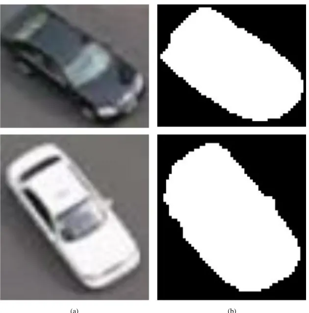
4.8 Example showing area of the vehicle regions (a) Vehicle region (b) Binary mask

from which area is estimated ...46

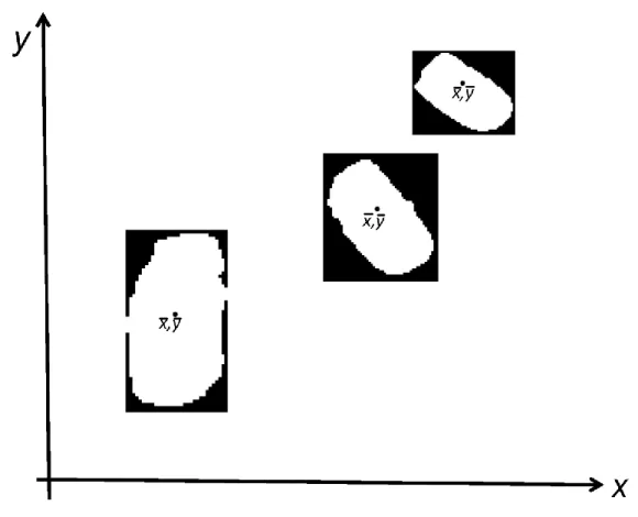
4.9 Example showing the location of centroid of vehicle regions ...47

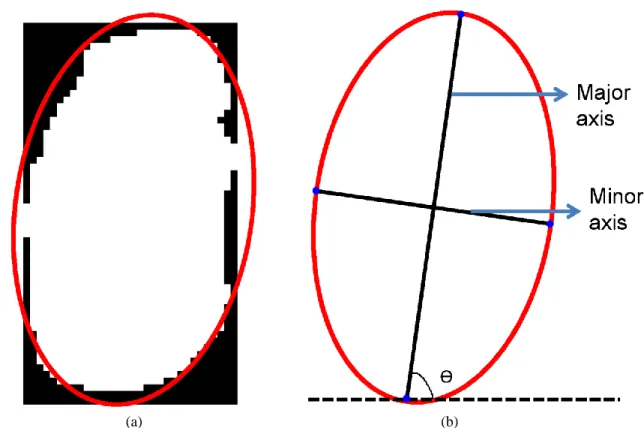
4.10 Example showing the orientation of the vehicle region (a) Vehicle region and its

corresponding ellipse (b) Graphical representation of the ellipse ...48

4.11 RGB to L

*

a

*

b

*

conversion (a) RGB image (b) Different scales of L

*

a

*

b

*

color

space ...50

4.12 Example frame at time t ...51

4.13 Regions extracted from Figure 4.12 ...51

(11)

xi

Figure

Page

4.17 Regions extracted from Figure 4.16...54

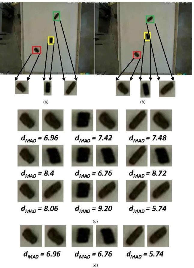
5.1 Example of HVS model analysis (a) Frame at time t (b) Frame at time t+1

(c) MAD index for different vehicle comparisons (d) MAD index for matching

vehicles ...56

5.2 Example of HVS model analysis (a) Frame at time t (b) Frame at time t+1

(c) MAD index for different vehicle comparisons (d) MAD index for matching

vehicles ...57

5.7 Overall similarity measure d for matched vehicles in I

t

and I

t+1

...64

5.8 Example showing tracked vehicles across different frames ...64

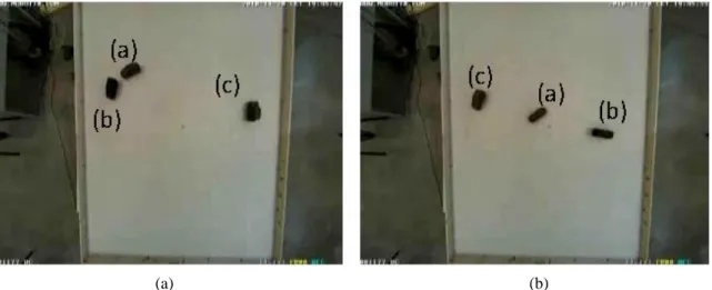
5.13 Example frames for showing the vehicle trajectory (a) Frame at time t (b) Frame at

time t+n ...69

5.14 Trajectory of the vehicles tracked from frame It to It+n ...69

5.15 Example frames for showing the vehicle trajectory (a) Frame at time t (b) Frame at

time t+n ...69

5.16 Trajectory of the vehicles tracked from frame I

t

to I

t+n

...70

5.17 Example of accident scenario (a) Frame before the occurrence of an accident (b)

Frame after occurrence of an accident ...75

(12)

xii

Figure

Page

5.18 Illustration of accident detection using change in area (a) Frame and its

corresponding binary image before occurrence of an accident (b) Frame and its

corresponding binary image after occurrence of an accident ...75

5.19 Illustration of accident detection using change in centroid (a) Binary image

showing centroid position of vehicles before accident (b) Binary image showing

centroid position of vehicles after accident ...76

5.20 Illustration of accident detection using change in orientation (a) Binary image

showing oreintation of vehicles before accident (b) Binary image showing

orientation of vehicles after accident ...76

5.21 Flowchart of the Accident Detection Algorithm ...77

5.22 Location of occurrence of accident ...77

6.1 Example frames from saigon01.avi used to determine threshold T ...81

6.2 Binary maps generated for frames shown in Figure 6.1 using different threshold

values ...81

6.3 Example frames from saigon02.avi used to determine threshold T ...83

6.4 Binary maps generated for frames shown in Figure 6.1 using different threshold

values ...82

6.5 Example showing failure in tracking using MAD index dMAD only ...85

6.6 Example showing failure in tracking using feature index d

features

only ...86

6.7 Some tracking results on saigon01 (a) Original frame (b) Ground Truth (c)

Segmentation (d) Tracking results ...88

6.8 Illustration of Vehicle Trajectory for Figure 6.7 (a) Start Frame (b) End Frame (c)

Vehicle trajectory obtained from algorithm (c) Temporal smoothness map ...88

6.9 Some tracking results on saigon01 (a) Original frame (b) Ground Truth (c)

6.10 Illustration of Vehicle Trajectory for Figure 6.9 (a) Start Frame (b) End Frame (c)

Vehicle trajectory obtained from algorithm (c) Temporal smoothness map ...89

(13)

xiii

6.12 Illustration of Vehicle Trajectory for Figure 6.11 (a) Start Frame (b) End Frame

(c) Vehicle trajectory obtained from algorithm (c) Temporal smoothness map90

6.14 Illustration of Vehicle Trajectory for Figure 6.13 (a) Start Frame (b) End Frame

(c) Vehicle trajectory obtained from algorithm (c) Temporal smoothness map92

6.15 Error Examples (a) Original Frame (b) Ground Truth (c) Segmentation (c) Error

Detection ...93

6.16 Error due to vehicle having low contrast with background ...93

6.17 Errors due to merging of vehicles ...94

6.18 Example of MSE (a) Frame at time t (b) Frame at time t+1 (c) MSE index for

different vehicle comparisons (d) MSE index for matching vehicles ...101

6.19 Different collision scenarios (a) Vehicles moving closely (b) Rear end collision by

the incoming vehicle (c) Side-on collision at intersection (d) Rear end collision by

the trailing vehicle (e) Side-on collision at turn (f) Side on collision from left (g)

Side-on collision from right (h) Multiple vehicle collision

(g) Normal tracking ...103

6.20 Illustration of accident detection system for various crash scenarios (a) Before

occurrence of accident (b) At point of accident (c) After accident ...106

6.21 Example of False alarm (a) Closely moving vehicles (b) Merged Blob (c) False

alarm raised by the system ...106

6.22 Performance Evaluation Terms ...107

(14)

1

CHAPTER 1

INTRODUCTION

1.1.Motivation

With the computation capability of the modern CPU processors, many complex real-time applications have been made possible and implemented in various fields worldwide. One of the widely used real-time applications is video surveillance systems. Video surveillance systems are been used for security monitoring, anomaly detection, traffic monitoring and many other purposes. Video surveillance systems have decreased the need of human presence to monitor activities captured by video cameras. And also one of the advantages of visual surveillance systems is videos can been stored and analyzed for future reference. One of the important applications of video surveillance systems is traffic surveillance. Extensive research has been done in the field of video traffic surveillance. Video traffic surveillance systems are used for vehicle detection, tracking, traffic flow estimation, vehicle speed detection, vehicle classification, etc. Video traffic surveillance has paved for numerous applications such as ATMS (Advanced Transportation Management Systems) [1] and (ITS) Intelligent Transportation Systems [2].

One of the widely used applications of traffic surveillance systems is vehicle detection and tracking. By detecting and tracking vehicles, we can detect vehicle’s velocity, trajectory, traffic density, etc. and if there is any abnormality, the recorded information can be send to the traffic authorities to take necessary action. The main advantage of the video monitoring systems over the existing systems such as physical detectors [3] that uses magnetic loops is the cost efficiency involved in installing and maintaining these video systems, and also the aspect of

(15)

2

video storage and transmission to analyze the detected events. Table 1.1 shows the performance comparison of various incident detection technologies. Thus video-based traffic surveillance systems have been preferred all over the world.

(16)

3

Having said the advantages of video-based traffic surveillance systems a new paradigm can be added to the application of video surveillance systems if we can detect accidents at traffic intersections and report the detected incident to the concerned authorities so that necessary action can be taken. Figure 1.1, shows some of the scenarios depicting traffic accidents and its consequences.

According to World Health Organization reports about 1.2 million lives are lost every year due to traffic accidents [5]. What is more amazing is the fact that traffic accident related deaths is one among the top ten causes of death worldwide, the list that includes tuberculosis, heart disease and AIDS as shown in Table 1.2. And also the cost of these accidents adds up to a shocking 1-3% of the world’s Gross National Product [6]. In United States, it is estimated that vehicle accidents account for over 40,000 deaths and cost over $164 billion each year. Among these, passenger- vehicle crashes account for the vast majority of deaths [7]. Without any preventive measures these figures are estimated to increase to 65% over the next 20 years. Studies have shown that the number of traffic related fatalities is highly dependent on emergency

(17)

4

response time [8]. When an accident occurs, response time is critical, every extra minute that it takes for help to arrive can mean the difference between life and death. So there arises a need for a system that can detect accidents automatically and report it to the concerned authorities quickly by which the emergency response time can be made faster, therefore potentially saving thousands of lives. With the usage of video-based traffic surveillance systems, accidents can be recorded and be sent to the traffic monitoring center so that the incoming traffic can be warned of an occurrence of accident and be diverted to avoid traffic congestion. This brings us to the motivation of this research. The motivation of this research is to develop an accident detection module at roadway intersections through video processing and report the detected accident along with the crash video to the concerned authorities, so that immediate action can be taken and potentially save thousands of live and property.

(18)

5

1.2.Research Goal and Challenges

1.2.1 Overview

Although considerable amount of research has been done to develop a system that can detect an accident through video surveillance, real-time implementation of all these systems have not been realized yet. Real-time implementation of accident detection through video-based traffic surveillance have always been challenging since one has to strike a right balance between the speed of the system and the performance of the systems such as correctly detecting accidents and also reducing false alarm rate. Ideally we want a system that could maximize the number of frames processed per second at the same time able to achieve acceptable performance rate. This brings us to the goal of this research. The goal of this research is to develop an accident detection module at roadway intersections through video processing that is suitable for real-time implementation. In this thesis we developed an accident detection module that uses the parameters extracted from the detected and tracked vehicles which is able to achieve good real-time performance.

An important stage in automatic vehicle crash monitoring systems is the detection of vehicles in each video frame and accurately tracking the vehicles across multiple frames. With such tracking, vehicle information such as speed, change in speed and change in orientation can be determined to facilitate the process of crash detection. As shown in the Figure 1.2, given the detected vehicles, tracking can be viewed as a correspondence problem in which the goal is to determine which detected vehicle in the next frame corresponds to a given vehicle in the current frame. While for a human analyst, the task of tracking can often be performed effortlessly, this task is quite challenging for a computer. Therefore in this thesis more emphasis has been given to the real-time implementation of vehicle detection and tracking.

(19)

6

1.2.1 Challenges in Vehicle Detection and Tracking

Implementing a system that does vehicle detection and tracking can be quite challenging. There are numerous difficulties that need to be taken into account, while implementing a system that performs vehicle detection and tracking. Figure 1.3 shows some of the scenarios encountered. Figure 1.3(a) shows frame captured at arbitrary time, Figure 1.3(b) shows the change in illumination conditions, Figure 1.3(c) shows change in weather conditions and Figure 1.3(d) shows change in traffic conditions. The following are the some of the challenges that can be faced while implementing real-time vehicle detection and tracking [9].

1. Vehicles can be of different size, shape and color. Furthermore, a vehicle can be observed from different angles, making the definition of a vehicle broader.

Figure 1.2: An example of vehicle tracking (a) Frame at time t (b) Frame at time t+1

(a) (b)

Figure 1.3: Scenarios showing different traffic conditions (a) Example frame (b) Change in illumination (c) Change in weather conditions (d) Change in traffic conditions (Images were

downloaded from http://i21www.ira.uka.de/image_sequences/)

(20)

7

2. Automatic segmentation of each vehicle from the background and from other vehicles so that all vehicles are detected.

3. Lightning and weather conditions vary substantially. Rain, snow, fog, daylight and darkness must all be taken into account when designing the system.

4. Vehicles can be occluded by other vehicles or structures.

5. Traffic conditions may vary, and many of the tracking algorithms degrade with heavy traffic congestion, where vehicles move slowly, and the distances between the vehicles are small.

6. Ability of the system to operate in real-time.

1.3.Methodology

The general description of the accident detection systems is presented below in the Figure 1.4.

(21)

8

In this thesis vehicle tracking is done based on low-level features and low-level human visual-system (HVS) modeling. Low-level features (e.g., color, orientation, size) are generally used because of their low computational complexity. Our method employs a weighted combination of low-level features along with a human vision based algorithm of visual dissimilarity for vehicle tracking. Although HVS models have found widespread use in a variety of consumer image processing applications, they have yet to be used extensively for vehicle tracking.

The detail description of the entire system is as follows: The first step of the process is the frame extraction step. In this frames are extracted from the video camera input. The second step of the process is the vehicle detection step. Here the already stored background frame is subtracted from the input frame to detect the moving regions in the frame. The difference image is further thresholded to detect the vehicle regions in the frame. Hence the vehicles in each frame are detected. In the third step low-level features such as area, centroid, orientation, luminance and color of the extracted vehicle regions are computed. And also for each of the region detected in frame at time t, similarity index is computed with all of the regions detected in frame at time

t+1 using human vision based model analysis. In the tracking stage, Euclidean distance is computed between the low-level features of each vehicle in frame n and all the other vehicles detected in frame n+1. This Euclidean distance vector is combined with the already computed similarity index for a particular vehicle region in frame n. Based on the minimum distance between vehicle regions tracking was done. In the next step, the centroid position of a tracked vehicle in each frame is computed and based on this information and the frame rate; the speed of the tracked vehicle is computed in terms of pixels/second. Since the position of the video camera is fixed, the camera parameters such as focal length, pan and tilt angle of the vehicle remains the constant and it can be computed using camera calibration algorithm. From all this information the pixel coordinates of the vehicle in each frame is converted to real-world coordinates. By this

(22)

9

conversion, the speed of the vehicle in terms of miles/hr is computed. Based on the velocity information, position and low-level features of the tracked vehicle suitable thresholds are defined to determine the occurrence of accidents. This is the overall description of the proposed system for accident detection at roadway intersections.

1.4.Contribution

The main contribution of this thesis is the real-time implementation of vehicle detection and tracking along with accident detection at roadway intersections. As discussed earlier although considerable amount of research has been done related to vehicle detection and tracking most of the systems fail to implement them in the real-time because of the complexity of the algorithm. In this thesis a new method have been adapted to track the detected vehicles in each video frame that is suitable for real-time implementation and also accident detection module have been added to vehicle detection and tracking module that can operate in real-time. We use the low-level features such as area, orientation, centroid, color, luminance of the extracted vehicle regions to achieve reasonable tracking rate. To determine accidents, speed, area and orientation of the tracked vehicle were used. The insight of this thesis is to process maximum video frames as possible and also achieve good performance rate simultaneously.

1.5.Thesis Organization

The rest of the thesis is organized as follows: Chapter 2 reviews the previous research work being done related to vehicle tracking and incident detection. In Chapter 3, the brief overview of the about the system, its advantages and limitations are discussed. Description of vehicle detection and feature extraction are presented in Chapter 4, results of vehicle tracking and accident detection are discussed in Chapter 5. Real-time performance evaluation and results of the algorithm are discussed in Chapter 6. Finally general conclusions and steps for future work are presented in Chapter 7.

(23)

10

CHAPTER 2

BACKGROUND

2.1. Overview

For the last two decades researchers have spend quality time to develop different methods that can be applied in the field of based traffic surveillance. Some of the applications of video-based surveillance include vehicle tracking, counting the number of vehicles, calculating vehicle velocity, finding vehicle trajectory, classifying the vehicles, estimating the traffic density, finding the traffic flow, license plate recognition, etc. Of late the focus of video-based traffic surveillance has shifted to detect incidents in roadways such as vehicle accidents, traffic congestion, and unexpected traffic blocks. From researches and surveys it was found that there is more necessity to detect accidents in highways and roadway intersections, as vehicle accidents causes huge loss to lives and property. Therefore the objective of video-based traffic surveillance of present is on accident detection in highways and intersections such that necessary action can be taken promptly without losing any quality time, so that lives of the injured can be saved. As discussed earlier the another advantage of video based surveillance is that the incidents can be recorded and analyzed for future reference and also the videos can be send to the traffic monitoring center to clear traffic congestion and divert the incoming traffic. One has to say for sure that the ultimate goal of video-based traffic surveillance is to pre-determine the accidents at highways and intersections and alert the incoming traffic of the occurrence of accident, which can potentially save thousands of lives and billions of dollars.

(24)

11

Apart from video-based systems, researches have also been done to detect incidents in roadways using other systems such as sensors, acoustic signal and others. These systems basically use physical detectors to collect the traffic parameters and apply machine learning and pattern recognition algorithm to detect the occurrence of an incident. Some of the techniques that had been used are decision trees for pattern recognition, time series analysis, Kalman filters and neural networks [10]-[18]. Spot sensors such as inductive loop sensors were employed by Gangisetty [19]. All of these systems showed varying amount of detection performance. But all the above described systems concentrated only on few areas of incident detection and failed to address the problem of traffic crashes at intersection. Only few systems [20] have addressed the problem of detecting crashes at intersection.

Green et al. [21] evaluated the performance of sound actuated video recording system which was used to analyze the reasons for traffic crashes at intersections. The system automatically records incident based on the sound it receives such as horns, clashing metal, squealing tires, etc. The results of this study were used by the transportation department to enhance the safety features by the traffic department which resulted in the reduction of accidents by 14%. Another system [22] developed a method to detect and report crashes at intersection using acoustic signal generated by the crashes. An acoustic database was developed which contains the normal traffic sounds, construction sounds and crash sounds and the system would compare the captured sound signal with the signals stored in the database to determine crashes. The system produced a good performance with false alarm rate of 1%. All the above studies suggested that there was a lot of scope for improvement to make these systems robust for different traffic flow conditions.

All the above described systems were able to detect incidents to certain extent; these systems can be employed for only a particular application. However the advantage of the utilizing the vision sensors for event recognition is their ability to collect diverse information such as

(25)

12

illegally parked vehicles, traffic violations, traffic jams and traffic accidents. Description of some of the vision based traffic applications can be found in [23]-[25]. Lai et al. [26] developed a system that is used to detect red light runners at intersections. There is lot more advantages of video based traffic accident detection system since the crashes can be recorded and analyzed and these recordings can be used to enhance the safety features at roadways and intersections. And importantly once the accident have been detected, the automated reporting of accident can be used to reduce the emergency response time which on its own makes the video based traffic surveillance systems superior to other non-vision based systems.

2.2. Traffic Image Analysis

There are basically four major steps involved in the video-based crash detection systems, various researches have been done on each individual section separately and good performance have been obtained. These are the following steps

1. Motion segmentation and vehicle detection 2. Vehicle tracking

3. Processing the results of tracking to compute traffic parameters 4. Accident detection using the traffic parameters

2.2.1. Motion segmentation and Vehicle Detection

Motion segmentation is the process of separating the moving objects from the background. The motion segmentation step is essential for detecting the vehicles in the image sequence. Figure 2.1 shows an example of vehicle detection. Figure 2.1(a) is the original image and Figure 2.1(b) shows the detected vehicle regions.

(26)

13

There are four main approaches to detect vehicle regions, they are

1. Frame differencing method 2. Background subtraction method 3. Feature based method

4. Motion based method

2.2.1.1. Frame Differencing Method

In the frame difference method moving vehicle regions are detected by subtracting two consecutive image frames in the image sequence. This works well in case of uniform illumination conditions, otherwise it creates non-vehicular region and also frame differencing method does not work well if the time interval between the frames being subtracted is too large. Some of the vehicle detection methods using this technique are described in detail in [27]-[30].

2.2.1.2. Background Subtraction Method

Background subtraction method is one of the widely used methods to detect moving vehicle regions. In this step the either the already stored background frame or the background generated from the accumulated the image sequence is subtracted from the input image frame to detect the moving vehicle regions. This difference image is then thresholded to extract the vehicle regions.

(a) (b)

(27)

14

The problem with the stored background frame is that they are not adaptive to changing illumination and weather conditions which may create non-existent vehicle regions and also works for stationary background. Therefore there is need to generate a background that is dynamic to the illumination and weather conditions. Various methods based on statistics and parametric model have been used. Some of the approaches [31] – [35] assumed Gaussian probability distribution for each pixel in the image. Then the Gaussian distribution model is updated with the pixel values from the new image frame in the image sequence. After enough information about model has been accumulated, each pixel (x, y) is classified either belonging to the foreground or background using the equation 2.1.

I(x, y) – Mean(x, y) < (C x Std (x, y)) (2.1)

where I(x, y) is pixel intensity, C is a constant, Mean(x, y) is the mean, Std (x, y) is the standard deviation.

Single Gaussian distribution based background modeling works well if the background is relatively stationary and it fails if the background contains shadows and non-important moving regions (e.g., tree branches). This led the researches to use more than one Gaussian (Mixture of Gaussians) to build more robust background modeling technique. In Mixture of Gaussian methods [36] – [37] colors from a pixel in a background object are described by multiple Gaussian distributions. These methods were able to produce good background modeling. In all the above described methods several parameters need to be estimated from the data to achieve accurate density estimation for background [38]. However most of the times these information is not known beforehand.

Non-parametric methods do not assume any fixed model for probability distribution of background pixels [39]-[40]. These methods are known to deal with multimodality in background pixel distributions without determining the number of modes in the background. However these

(28)

15

systems does not adapt to sudden changes in illumination. So few methods based on Support Vector Machine (SVM), robust recursive learning were proposed to dynamically update the background [41]-[43]. Some methods [44] - [45] used Kalman filter to model the foreground and background and some other methods [46]-[47] used depth and color information to model the background using stereo camera. Background subtraction methods produced better segmentation results due to better background modeling, when compared to frame differencing method. But the disadvantages of background modeling to detect vehicle regions are high computational complexity making them difficult to operate in real-time and increased sensitivity to changes in lightning conditions.

2.2.1.3. Feature Based Method

Since the background subtraction methods needs accurate of modeling of background to detect moving vehicle regions, researched shifted their focus to detect moving vehicle regions using feature based methods. These methods made use of sub-features such as edges or corner of vehicles. These features are then grouped by analyzing their motion between consecutive frames. Thus a group of features now segments a moving vehicle from the background. The advantages of these methods [48] is that the problem of occlusion between the vehicle regions can be handled well, the feature based methods have less computational complexity compared to background subtraction method, the sub-features can be further analyzed for classifying the vehicle type and there is no necessity of stationary camera. Koller et al. [49] used displacement vectors from the optical flow field and edges as sub-features for vehicle detection. Beymer et al. [3] used corner of vehicles as features for measuring traffic parameters. Edges are used as features to detect vehicles by Dellart et al. [50]. Smith [51] used combination of corners and edges to detect moving vehicles. But the disadvantage of these systems is that if the features are not grouped accurately, then there may be failure in detecting vehicles correctly and also some of the systems are computationally complex and needs fast processing computers for real-time implementation.

(29)

16

2.2.1.4. Motion Based Method

Motion based approaches were also used to detect the vehicle regions in image sequences [38]. Optical flow based approaches were used to detect moving objects in the methods [52]-[53]. These methods are very effecting on small moving objects. Wixon [54] proposed an algorithm to detect salient motion by integrating frame-to-frame optical flow over time; thus it is possible to predict the motion pattern of each pixel. This approach assumes that the object tends to move in a consistent direction over time and that foreground motion has different saliency. The drawbacks of optical flow based methods are calculation of optical flow consumes time and the inner points of a large homogeneous object (e.g. car with single color) cannot be featured with optical flow. Some of the approaches used spatio-temporal intensity variations [43, 55] to detect motion and thus segment the moving vehicle regions.

2.2.2. Camera Calibration

Once the vehicle regions are detected and suitable features such as area, orientation, color, etc. are calculated, it is necessary for the 2D information obtained from the image to be mapped to the 3D information with respect to the real-world. Geometric camera calibration is the process of determining the 2D-3D mapping between the camera and the world coordinate systems [56]. Therefore there is a need to convert the camera coordinates to world coordinates using the internal (principal point, focal length, aspect ratio) and external parameters of the camera (position and orientation of camera in world coordinate system). We can classify the camera calibration techniques in two types: photogrammetric calibration and self-calibration. In photogrammetric calibration [57], an object whose 3D world coordinates is known in prior is observed by a camera to find the calibration parameters. In self calibration techniques [58], the position of the camera is changed to record static scenes and image with known internal

(30)

17

parameters, from which calibration parameters can be recovered. Figure 2.2 shows imaging geometry for perspective transformation.

Earlier research related to camera calibration employed full-scale non-linear optimization [60]-[62]. Good accuracy has been achieved using these methods, but the disadvantage of these methods is that they require a good initial guess and a computationally intensive non-linear search. Although the equations governing the transformation from 3D world coordinate to 2D image coordinate are nonlinear functions of intrinsic and extrinsic camera parameters, they are linear if lens distortion is ignored. By this assumption perspective transformation matrix can be computed using linear equations [63]-[65]. The main advantage of these methods is that they eliminate non-linear optimization. However, lens distortion cannot be modeled using these methods. If images are taken by the same camera with fixed internal parameters, correspondences between three images are sufficient to recover both the internal and external parameters [66]-[67]. Bu the disadvantage of these methods is they require a large number of features to achieve robustness.

(31)

18

Worall et al. employed an interactive tool for calibrating a camera that is suitable for use in outdoor scenes [68]. Wang and Tsai [69] used vanishing point technique to calibrate traffic scenes. Bas and Crisman [70] used the known height and tilt angle of the camera for calibration using a single set parallel line drawn by the user along the road edges while Lai [71] used an additional line of know length perpendicular to the road edges to remove the restriction of known height and tilt angle of the camera. Fung et al. [72] developed a method that is robust against small perturbations in markings along the roadside. The above described methods works well if the camera is static and fails if the position of the camera is changed.

To overcome the problems of calibration when the position of the camera is changed automatic calibration techniques were used. Daily et al. [73] relate pixel displacement to real-world units by fitting a linear function to scaling factors obtained using a known distribution of typical length of vehicles. Schoepflin and Dailey [74] calibrated PTZ cameras using lane activity maps which are computed by frame-differencing. Zhang et al. [75] used three vanishing point method to estimate the calibration parameters.

2.2.3. Vehicle Tracking

Once the vehicle regions are detected it is necessary for these vehicle regions to be tracked in the image sequences so that necessary information about the vehicle such as speed, vehicle trajectory, vehicle dimensions can be computed and used for further use. An illustration of vehicle tracking is shown in Figure 2.3. Figure 2.3(a) shows frame at time t, Figure 2.3(b) shows frame at time

t+1 and Figure 2.3(c) shows frame at time t+2. In these figures, the bounding box around each vehicle is same indicating that the vehicles are tracked correctly.

(32)

19

Vehicle tracking is an important stage in crash detection systems. Given the detected vehicles, tracking can be viewed as a correspondence problem in which the goal is to determine which detected vehicle in the next frame corresponds to a given vehicle in the current frame. Over the years various researches have been conducted related to vehicle tracking. These approaches can be classified as follows.

1. Region-Based Tracking 2. Active Contour Tracking 3. 3D Model-Based Tracking 4. Markov Random Field Tracking 5. Feature- Based Tracking

6. Color and Pattern-Based Tracking 7. Other approaches

2.2.3.1. Region-Based Tracking

In this method image frame containing vehicles is subtracted from the background frame which is then further processed to obtain vehicle regions (blobs). Then these vehicle regions are tracked. Various methods have been proposed based on this approach [73, 76, 77]. Gupte et al. [76] proposed a method that performed vehicle tracking at two levels: region level and vehicle level. The method is based on the establishment of correspondences between regions and vehicles as the

Figure 2.3: Illustration of vehicle tracking (a) Frame at time t (b) Frame at time t+1 (c) Frame at time t+2

(33)

20

vehicle move through the image sequence using maximally weighted graph. Bu the disadvantage of these methods is that they have difficulty in handling shadows, occlusion.

2.2.3.2. Active Contour Tracking

The next approach used to track vehicles was tracking the contours representing the boundary of the vehicle [78]-[79]. These are known as active contour models or snakes. Once the vehicle regions are detected in input frame the contours of the vehicle are extracted and dynamically updated in each successive frame. In the method used by Koller et al. [78] the vehicle regions are detected by background subtraction and tracked using intensity and motion boundaries of the vehicle objects. This method makes use of Kalman filters for estimating the affine motion and the shape of the contour. The advantage of active contour tracking over region-based tracking is the reduced computational complexity. But the disadvantage of the method is their inability to accurately track the occluded vehicles and tracking need to be initialized on each vehicle separately to handle occlusion better.

2.2.3.3. 3D Model-Based Tracking

In 3D model-based tracking [80]-[84] localize and track vehicle by matching a projected 3D model to the image data. Tan et al. [85]-[86] proposed a generalized Hough transformation algorithm based on single characteristic line segment matching an estimated vehicle pose and also analyzed the one-dimensional correlation of image gradients and determine the vehicle pose by voting. Pece et al. [87] presented a statistical Newton method for the refinement of the vehicle pose. The advantages of 3D model-based vehicle tracking is they are robust to interference between nearby images and also be applied to track vehicles which greatly change their orientations. But on the downside these models have high computational cost and they need detailed geometric object model to achieve high tracking accuracy.

(34)

21

2.2.3.4. Markov Random Field Tracking

Kamijo et al. [88] proposed a method to segment and track vehicle using spatiotemporal Markov random field. In this method the image is divided into pixel blocks and spatiotemporal Markov random field is used to update an object map using current and previous image. This method handled occlusions well. But the drawback of this method is that it does not yield 3Dinformation about vehicle trajectories in the world coordinate system. In addition in order to achieve accurate results the image in the sequence are processed in reverse order to ensure that vehicles recede from the camera. The accuracy decreased by a factor of two when the sequence is not processed in reverse, thus making the algorithm unsuitable for on-line processing.

2.2.3.5. Feature-Based Tracking

In feature-based tracking [78], [89]-[92] suitable features are extracted from the vehicle regions and these features are processed to track the vehicles correctly. These algorithms have low complexity and can operate in real-time and also can handle occlusions well. Beymer et al. [3] used feature tracking method in which the vehicle point features are tracked throughout the detection zone (entry and exit region). The feature grouping is done by constructing a graph over time, with vertices representing sub-feature tracks and edges representing the grouping relationships between tracks. Kanhere et al. [89] used 3D world coordinates of the feature point of the vehicle and grouped those points together in order to segment and track the individual vehicles. Texture-based features were used for tracking in [92]. Scale-Invariant features were used for tracking by Choi et al. [93]. The drawback of feature-based tracking is the recognition rate of vehicles using tow-dimensional image features is low, because of the non-linear distortion due to perspective projection and the image variations due to movement relative to the camera.

(35)

22

2.2.3.6. Color and Pattern-Based Tracking

Chachich et al. [94] used color signatures in quantized RGB space for tracking vehicles. In this work, vehicle detections are associated with each other by using a hierarchical decision process that includes color information, arrival likelihood and driver behavior. In [95], a pattern-recognition based approach to on-road vehicle detection has been studied in addition to tracking vehicles from a stationary camera. But the tracking based on color and pattern matching is not that reliable.

2.2.3.7. Other Approaches

The other approaches that were used for vehicle tracking includes optical flow based tracking [36, 51, 96], Markov Chain Monte Carlo based tracking [96] and Kalman-Filtering based tracking [97].

2.2.4 Accident Detection Systems

After vehicles in image sequence are detected and tracked correctly suitable traffic parameters (e.g. speed, trajectory, traffic flow) are extracted from the vehicle, the computer traffic parameters are used to detect incidents at highways and roadway intersections. Many research works have been done in the past to address this problem as there are numerous advantages in detecting accidents. Earlier researches related to traffic accident detection system involved detecting abnormal incidents such as traffic jam, detecting fallen-down obstactles, etc. Ikeda et al. [98] proposed an image processing based automatic abnormal incident detect system. The system is used to detect four types of incidents namely stopped vehicles, slow vehicles, fallen objects and vehicles that have attempted lane successive changes. Kimachi et al. [99] studied about vehicle behaviors causing incidents (e.g. traffic accident) using image processing techniques and fuzzy logic to predict an incident before it occurs. Trivedi et al. [100] described a method for developing distributed video networks for incident detection and management using

(36)

23

omnidirectional camera. Blosseville et al. [101] used image processing technique to detect shoulder incidents. Versavel and Boucke [102] presented a video incident detection method that used PTZ cameras. Michalopoulos and Jacobson [103] developed a method to detect incidents almost 2miles away. These methods were able to detect incidents to good extent with false alarm rate of about 3%. However most of these systems were used to detect incidents at roadways and have limited ability to detect traffic accidents at intersection.

Some of the approaches discussed above were limited to detect abnormal incidents at roadways; therefore more emphasis was given to determine accidents by later researchers. Atev et al. [104] used vision-based approach to predict collision at traffic intersection. In this method the vehicles are tracked using their centroid position and information about the vehicle such as velocity, position, width and height are computed and a bounding box is drawn around each tracked vehicle. Using the bounding box information around each vehicle collision is determined based on the amount to which the bounding box intersect. Hu et al. [105] used vehicle velocity and trajectory information to predict traffic accident using neural networking training of traffic parameters. Ki and Lee [106] used variation in speed, area, position and direction of the tracked vehicle to obtain and accident index which would determine the occurrence of accident at intersections. The method produced correct detection rate of 50% and false alarm rate of 0.00496% on their test conditions. Kamijo et al. [107] applied a simple left-to-right hidden Markov model to detect accident at traffic intersections. The system is able to determine three types of incident namely bumping accident, passing and jamming. However the conclusion was restrictive because there were not enough traffic accident data. Salim et al. [114] used speed, angle, position, direction, size of the tracked vehicle and using learning algorithm to detect collision at road intersections. Althoff et al. [117] used Markov chain probability model to detect collision. Zou et al. [118] used HMM to detect incidents at signaled intersection using modeled traffic parameters. How the disadvantage of these methods is that some algorithm need high level

(37)

24

learning algorithm that are computationally complex and may not feasible to be implemented in real-time.

2.3 Limitations of existing Vehicle Tracking and Accident Detection Systems

Someof the limitations of the existing vehicle detection, tracking and accident detection systems are given below

1. Most of the existing vehicle detection and tracking systems have high computational complexity

2. Some of the vehicle detection systems use sophisticated background modeling methods which adds to the complexity of the algorithm.

3. Some of the existing vehicle tracking systems need high speed processors for implementation.

4. Some of the systems make use of high level learning algorithm such as HMM, neural network to detect accidents which make the real-time implementation difficult.

5. Real-time implementation of these systems is not feasible on low speed processors

In this chapter we have briefly discussed about the existing vehicle tracking and accident detection systems and their advantages and disadvantages. Considerable number of research work has been done related to this field and few systems have been used in practical situations. However there is room for improvement in all the systems that have been reviewed

(38)

25

CHAPTER 3

SYSTEM OVERVIEW AND CAMERA CALIBRATION

3.1. Problem Definition

The problem addressed in this research is preliminary approach to real -time implementation of accident detection systems at traffic intersections. Therefore the main objective of this research is to design and implement an accident detection system through video processing that is suitable for real-time implementation. Figure 3.1 illustrates brief overview of the system.

Figure 3.1: Brief overview of the accident detection system [accident image shown in the figure is downloaded from http://www.fotosearch.com/GLW051/690397494/]

(39)

26

3.2. Approach

As shown in the Figure 3.1, image sequences are extracted from the video camera mounted on the pole at traffic intersection. The image sequences are fed to the accident detection module system where the occurrence of the accident is determined. The accident detection system consists of vehicle detection, vehicle tracking, vehicle parameter extraction and accident detection sections. The brief overview of the accident detection module is presented in detail in chapter 1, section 1.3. In addition to the image input, some more auxiliary information is also fed as input to the system. The following information is fed as input to the system. They are: stored background image, threshold values for the image processing, information about the position and orientation of the camera, camera calibration parameters and frame rate of the video sequence. After analyzing the image sequence, the system identifies the moving vehicles in the image and tracks them using low-level features. After the vehicles are tracked correctly in each frame, the speed, orientation, position and area of the tracked vehicle are used to determine the occurrence of accident. Once an occurrence of accident is detected, the system signals the detection of accident to the user.

3.2.1. Advantages of the System

The following are the advantages of the system

1. System is able to operate in real-time with common CPU processor and with the use of high speed processor; the processing rate can be speeded up further.

2. The vehicle detection and tracking algorithm used in the system have low computational cost.

3. Vehicle tracking method used in the system makes use of low-level features which have low complexity when compared to the existing systems discussed earlier

(40)

27

4. The system focuses on real-time implementation of accident detection at traffic intersection where the occurrence of accidents is estimated to be more.

5. Because of the fast operating time, future enhancements can be added to the system to make it more robust.

3.2.1. Limitations and Assumptions

The following list the limitations and assumptions used in the thesis

1. The system assumes that the video camera used to record the traffic image sequence is assumed to be parallel to the ground plane.

2. The system works well only in daylight conditions. The performance of the system has not been evaluated in night conditions.

3. The system does not handle occlusion well especially if part of a vehicle is occluded with another vehicle.

4. Although the system is able to achieve real-time performance, the method had been tested and evaluated offline. Online evaluation of the algorithm has not been done.

3.3. Experimental Setup and Testing Conditions

For the purpose of testing our algorithm we used two video sequences obtained from traffic intersection at Saigon, Vietnam. These videos were used to test the performance of the tracking algorithm. These videos were used as they provided nice scenarios for busy traffic intersection. The testing was done offline and results were used to improve the performance of the tracking algorithm. Few frames from the test videos are shown in the Figure 3.2 and Figure 3.3. Figure 2.4 shows the frame sequences from the video named saigon01.avi and Figure 2.5 shows the frame sequences from the video named saigon02.avi.

(41)

28

Figure 3.2: Frame sequences from test video saigon01.avi

(42)

29

3.3.1. Indoor Experimental Setup

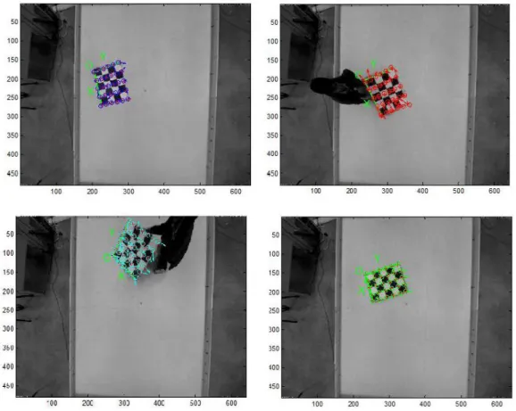
For the purpose of testing the accident detection system, indoor experimental setup was made in the laboratory with artificial lighting mimicking daylight conditions. The video camera used for this purpose was Q24 Mobitix Camera. The camera was placed parallel to the ground plane to shoot the testing sequence. PC controlled cars were used for the purpose of tracking vehicles and creating collision between vehicles. The advantage of PC controlled cars is that the trajectory and the velocity of the vehicles can be controlled by the user. Optical tracking system was also used in the setup. The advantage of Optical tracking system is that the velocity information of the vehicles can be obtained instantaneously which is used to verify the velocity information determined by the accident detection system. Figure 3.4 shows the experimental setup used in the laboratory.

(43)

30

Figure 3.5 shows the frame sequence in the testing video obtained from the laboratory setup. The bottom row shows a scenario for occurrence of accident.

The algorithm for vehicle detection, vehicle tracking and accident detection system are explained in detail in the following chapters. The detail description of vehicle detection is presented in Chapter 3.

3.4. Camera Calibration

Camera Calibration is an essential step in a vision-based vehicle tracking system. Camera calibration involves estimating a projective matrix which describes the mapping of points in the world onto the image plane. A calibrated camera enables us to relate pixel-measurements to measurements in real world units (e.g., feet) which are used to handle scale changes (as vehicles

(44)

31

approach or recede from the camera) and to measure speeds [108]. Two types of parameters need to be estimated to find the mapping between the image coordinates and world coordinates. They are extrinsic and intrinsic parameters of the camera. The extrinsic parameters define the location and orientation of the camera reference frame with respect to a known world reference frame. The intrinsic parameters are necessary to link the pixel coordinates of an image point with the corresponding coordinates in the camera reference plane [109]. Figure 3.6 shows mapping of 3D point to 2D point.

3.4.1. Calibration for Saigon Traffic Videos

For the Saigon videos the camera is assumed to be placed parallel to the ground plane since accurate information about the camera position is not known. From close observation of the traffic video it was estimated that the camera was placed at very high angle, presenting good

(45)

32

down view of the traffic intersection. Figure 3.7 shows the scenario encountered in case of Saigon

traffic intersection. The camera is place parallel to the ground plane.

3.4.1.1. Photogrammetric correction factor

Since the sizes of the objects in an image are measured in pixels, they have to be converted into units used in the real world to determine the sizes and speeds of vehicles to which they correspond [48]. The Figure 3.8 illustrates the situation where the camera is place parallel to the ground plane.

From the image geometry shown in Figure 3.7

𝑦 𝑥 =

𝑑2

𝑑1 = 𝑐𝑜𝑛𝑠𝑡𝑎𝑛𝑡 (3.1) Figure 3.7: Camera placed parallel to the ground plane

(46)

33 𝑥 = 𝑑1

𝑑2 × 𝑦 (3.2) where (d1/d2) = scale factor

In this case, the actual distance can be calculated by multiplying the distance in pixels by the scale factor. Similarly, the area of a blob can be calculated using the scale factor.

3.4.2. Camera Calibration for Q24 Mobitix Camera

A perspective-projective pinhole camera model is assumed. The relationship between an object point measured with respect to user-defined world coordinate system and its image plane is described by a 3x4 homogeneous transformation matrix [108]. The detailed description of the intrinsic and extrinsic parameters can be found in [109,110,111].This matrix will be referred as the camera calibration matrix C, where C = CinCext. Cin is the matrix containing the intrinsic parameters and Cext is the matrix containing the extrinsic parameters.

(47)

34

The matrix containing the intrinsic camera parameters is given by:

𝐶_𝑖𝑛 = −𝑓 𝑠_𝑥 0 𝑜𝑥 0 −𝑓 _𝑠_𝑦 𝑜_𝑦 0 0 1 (3.3)

where f is the focal length of the camera. [sx sy] correspond to the effective size of the pixels in the horizontal and vertical directions (in millimeters). [ox oy] are the coordinates of the principal point (in pixels).

The matrix containing the extrinsic camera parameters is given by:

𝐶_𝑒𝑥𝑡 =

𝑟₁₁ 𝑟₁₂ 𝑟₁₃ −𝑅₁𝑇𝑇 𝑟₂₁ 𝑟₂₂ 𝑟₂₃ −𝑅₂𝑇𝑇 𝑟₃₁ 𝑟₃₂ 𝑟₃₃ −𝑅₃𝑇𝑇

(3.4)

where T is the translation vector and R is the rotation matrix given by

𝑅 =

𝑟₁₁ 𝑟₁₂ 𝑟₁₃ 𝑟₂₁ 𝑟₂₂ 𝑟₂₃

𝑟₃₁ 𝑟₃₂ 𝑟₃₃ (3.5)

𝑝 = 𝐶𝑃 (3.6)

where 𝑝 = 𝑢𝑤 𝑣𝑤 𝑤 and 𝑃 = 𝑥 𝑦 𝑧 𝑇_{are vectors containing homogeneous coordinates of} image point, 𝑝 = 𝑢 𝑣 and world point 𝑃 = 𝑥 𝑦 𝑧 𝑇_{respectively. Representing the matrix with} corresponding entries we get

𝑢𝑤 𝑣𝑤 𝑤 =

𝑐₁₁ 𝑐₁₂ 𝑐₁₃ 𝑐₁₄ 𝑐₂₁ 𝑐₂₂ 𝑐₂₃ 𝑐₂₄ 𝑐₃₁ 𝑐₃₂ 𝑐₃₃ 𝑐₃₄

𝑥 𝑦 𝑧 1 (3.7)

The homogeneous transformation matrix C is unique only up to a scale factor. C by making the scale factor c34 = 1.

(48)

35 Expanding the above equation (3.7), yields

𝑢 = 𝑐11𝑥+𝑐12𝑦 +𝑐13𝑧+𝑐14𝑥

𝑤 (3.8)

𝑣 = 𝑐21𝑥+𝑐22𝑦+𝑐23𝑧+𝑐24𝑥

𝑤 (3.9) 𝑤 = 𝑐₃₁𝑥 + 𝑐₃₂𝑦 + 𝑐₃₃𝑧 + 1 (3.10)

Substituting w into two equations (3.8) and (3.9) gives

𝑢 =𝑐11𝑥+𝑐12𝑦+𝑐13𝑧+𝑐14𝑥

𝑐31𝑥+ 𝑐32𝑦 + 𝑐33𝑧+1 (3.11)

𝑣 = 𝑐21𝑥+𝑐22𝑦+𝑐23𝑧+𝑐24𝑥

𝑐₃₁𝑥+ 𝑐₃₂𝑦 + 𝑐₃₃𝑧+1 (3.12)

Equations (3.8) and (3.9) define a mapping from the world coordinates to the image coordinates.

For a point in the world, we can calculate its image coordinates if we know the location of that point in terms of the user-defined world-coordinate system and camera calibration matrix,

C. The camera calibration matrix C consists of 11 unknown parameters. Knowing the world coordinates and the image coordinates of a single point yields to equations of the form (3.8) and (3.9). Six or more points in a non-degenerate configuration lead to an over-determined system:

𝑥₁ 𝑦₁ 𝑧₁ 1 0 0 0 0 −𝑢₁𝑥₁ −𝑢₁𝑦₁ −𝑢₁𝑧₁ 0 0 0 0 𝑥₁ 𝑦₁ 𝑧₁ 1 −𝑣₁𝑥₁ −𝑣₁𝑦₁ −𝑣₁𝑧₁ 𝑥₂ 𝑦₂ 𝑧₂ 1 0 0 0 0 −𝑢₂𝑥₂ −𝑢₂𝑦₂ −𝑢₂𝑧₂ 0 0 0 0 𝑥2 𝑦2 𝑧2 1 −𝑣2𝑥2 −𝑣2𝑦2 −𝑣2𝑧2 . . . . . . . . . . . . 𝑥_𝑛 𝑦_𝑛 𝑧_𝑛 1 0 0 0 0 −𝑢_𝑛𝑥_𝑛 −𝑢_𝑛𝑦_𝑛 −𝑢_𝑛𝑧_𝑛 0 0 0 0 𝑥_𝑛 𝑦_𝑛 𝑧_𝑛 1 −𝑣_𝑛𝑥_𝑛 −𝑣_𝑛𝑦_𝑛 −𝑣₁𝑧₁ 𝑐₁₁ 𝑐₁₂ 𝑐₁₃ 𝑐₁₄ 𝑐₂₁ . . . 𝑐₃₃ = 𝑢₁ 𝑣₁ 𝑢₂ 𝑣₂ . . . 𝑢_𝑛 𝑣_𝑛 (3.10)