Incremental and Adaptive L1-Norm Principal Component Analysis: Novel Algorithms and Applications

(1)

Theses

7-2018

Incremental and Adaptive L1-Norm Principal

Component Analysis: Novel Algorithms and

Applications

Mayur Dhanaraj

[email protected]

Follow this and additional works at:https://scholarworks.rit.edu/theses

This Thesis is brought to you for free and open access by RIT Scholar Works. It has been accepted for inclusion in Theses by an authorized administrator of RIT Scholar Works. For more information, please [email protected].

Recommended Citation

Dhanaraj, Mayur, "Incremental and Adaptive L1-Norm Principal Component Analysis: Novel Algorithms and Applications" (2018). Thesis. Rochester Institute of Technology. Accessed from

(2)

Component Analysis: Novel Algorithms and

Applications

by

Mayur Dhanaraj

A Thesis Submitted in Partial Fulfillment of the Requirements for the Degree of Master of Science in Electrical Engineering

Supervised by Dr. Panos P. Markopoulos

Department of Electrical and Microelectronic Engineering Kate Gleason College of Engineering

Rochester Institute of Technology, Rochester, New York July 2018

Approved by:

Dr. Panos P. Markopoulos, Assistant Professor

Thesis Advisor, Department of Electrical and Microelectronic Engineering

Dr. Andreas Savakis, Professor

Committee Member, Department of Computer Engineering

Dr. Sohail A. Dianat, Professor

Committee Member, Department of Electrical and Microelectronic Engineering

Dr. Sohail A. Dianat, Professor

(3)

Rochester Institute of Technology Kate Gleason College of Engineering

Title:

Incremental and Adaptive L1-Norm Principal Component Analysis: Novel Algorithms and Applications

I, Mayur Dhanaraj, hereby grant permission to the Wallace Memorial Library to repro-duce my thesis in whole or part.

Mayur Dhanaraj

(4)

(5)

Dedication

I dedicate this work to my mother Dr. Gnaneswari Gopal, my sisters Mrunalini Rout and Mrudula Dhanraj, my grandfather K. Gopal Naidu and my best friends Prakruthi Manjunath, Prasidh P Kumar and Akash M Bushan for their continued love and support. I

also dedicate this work to my late father Dhanaraj Guntoor Muniswamy, my late paternal aunt Amruthamma M and my late maternal uncle Sumanth Kumar for their blessings. Last but not the least I dedicate this work to the almighty for giving me the strength and

(6)

Acknowledgments

There are a number of people without whom this thesis might not have been possible, and to whom I am forever indebted.

To my mother, Dr. Gnaneswari Gopal for giving birth to me and nurturing me, for being a pillar of my family and for her constant support and advice. I would not be who I am today without her support. A very special thanks to you mother.

To my advisor and mentor, Dr. Panos P. Markopoulos for being an excellent guide, a patient listener, an inspiration and an extraordinary teacher. Thank you professor.

I thank each member of my family for being very supportive to me throughout my life. I thank Mr. Mahesh Narayana for constantly encouraging me with his words of wisdom. I thank my fellow lab partners Dimitis Chachlakis and Ruslan Dautov (both PhD students), for their invaluable advice whenever needed.

I thank Dr. Sailaja Viswanath and Dr. T. M. Manjunath for their invaluable support to my mother in times of need.

I also thank my thesis committee members Dr. Andreas Savakis and Dr. Sohail A. Dianat for taking their valuable time to review my thesis and for their invaluable suggestions that led to the betterment of this thesis.

(7)

Abstract

Incremental and Adaptive L1-Norm Principal Component Analysis: Novel Algorithms and Applications

Mayur Dhanaraj

Supervising Professor: Dr. Panos P. Markopoulos

L1-norm Principal-Component Analysis (L1-PCA) is known to attain remarkable resis-tance against faulty/corrupted points among the processed data. However, computing L1-PCA of “big data” with large number of measurements and/or dimensions may be com-putationally impractical. This work proposes new algorithmic solutions for incremental and adaptive L1-PCA. The first algorithm computes L1-PCA incrementally, processing one measurement at a time, with very low computational and memory requirements; thus, it is appropriate for big data and big streaming data applications. The second algorithm combines the merits of the first one with additional ability to track changes in the nominal signal subspace by revising the computed L1-PCA as new measurements arrive, demon-strating both robustness against outliers and adaptivity to signal-subspace changes. The proposed algorithms are evaluated in an array of experimental studies on subspace esti-mation, video surveillance (foreground/background separation), image conditioning, and direction-of-arrival (DoA) estimation.

(8)

List of Contributions

• Novel Algorithm for Incremental L1-norm Principal-Component Analysis. • Novel Algorithm for Adaptive L1-norm Principal-Component Analysis.

• Numerical Studies on Outlier-Resistant Signal Subspace Estimation and Tracking. • Experimental Studies on Image Conditioning, Specifically Glare/Shadow Artifacts

Removal from Face Images.

• Experimental Studies on Video Background/Foreground Extraction.

• Experimental Studies on Jammer-Resistant Direction-of-Arrival (DoA) Estimation and Tracking.

• Publications:

1) P. P. Markopoulos, M. Dhanaraj and A. Savakis, "Algorithms for incremental and adaptive L1-norm principal-component analysis",IEEE J. Sel. Top. Signal Process (under revision).

2) M. Dhanaraj and P. P. Markopoulos, "Novel algorithm for incremental L1-norm principal-component analysis", IEEE/EURASIP Euro. Signal Process. Conf. (EU-SIPCO 2018), Rome, Italy, Sept. 2018 (to appear).

(9)

List of Tables

(12)

List of Figures

1.1 Projection error minimization PCA. . . 3

1.2 Projection variance maximization PCA. . . 4

1.3 Line-fitting for nominal data. . . 6

1.4 Line-fitting for outlier-corrupted data. . . 6

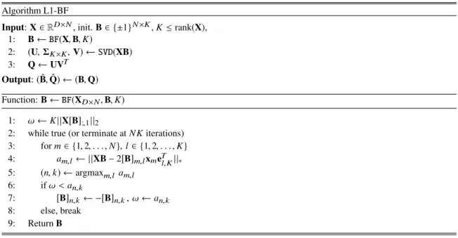
2.1 Pseudocode of L1-BF algorithm. . . 13

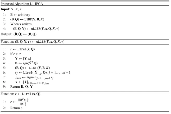
3.1 Pseudocode of proposed L1-IPCA algorithm. . . 19

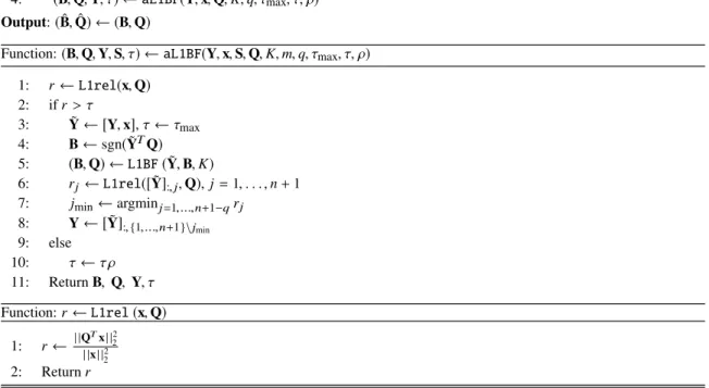
3.2 Pseudocode of proposed L1-APCA algorithm. . . 24

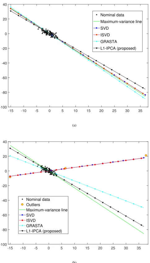
4.1 Line-fitting experiment. PC calculation on (a) clean/nominal and (b) outlier-corrupted data;N = 100,D= 2,K = 1,n=10, andτ=0.85. . . 26

4.2 Subspace estimation experiment. Average normalized subspace error ver-sus update indexi;D=5, N = 200,K = 1;n= 20,τ=0.66. . . 28

4.3 Subspace estimation experiment. Frequency of success versus update indexi. 30 4.4 Subspace estimation experiment. Average time versus update indexi. . . . 30

4.5 Subspace tracking experiment. Average normalized subspace error versus adaptation indexi;D = 5, N = 250,K = 1;n = 20, τmax = 0.8, ρ = 0.35 andq =0.75n; Subspace change after 130−npoints. . . 33

4.6 Subspace tracking experiment. L1-reliability thresholdτiversus adaptation indexi. . . 33

4.7 Subspace tracking experiment. Frequency of success versus adaptation in-dexi. . . 35

4.8 Subspace tracking experiment. Average time versus adaptation indexi. . . . 35

4.9 Image conditioning experiment. (a) Original face image with glare and shadows. Image conditioned with (b) ISVD [62], (c) the method of [64], (d) GRASTA [82], (e) PCP [19], (f) OR-PCA [73, 74], (g) the method of [49], (h) the method of [47] and (i) L1-IPCA (proposed). . . 37

4.10 Image conditioning experiment. (a) Original face image with glare and shadows. Image conditioned with (b) ISVD [62], (c) the method of [64], (d) GRASTA [82], (e) PCP [19], (f) OR-PCA [73, 74], (g) the method of [49], (h) the method of [47] and (i) L1-IPCA (proposed). . . 38

(13)

4.11 Time consumed for image conditioning . . . 39 4.12 Video processing experiment – video 1. (a) Original frame. Background

extracted by (b) ISVD [62], (c) GRASTA [82], (d) PCP [19], (e) OR-PCA [74], (f) RPCA [29], (g) ReProCS [72], (h) method of [47], and (i) L1-IPCA (proposed). Foreground extracted by (j) ISVD [62], (k) GRASTA [82], (l) PCP [19], (m) OR-PCA [74], (n) RPCA [29], (o) ReProCS [72], (p) method of [47], and (q) L1-IPCA (proposed). . . 42 4.13 Video processing experiment – video 2. (a) Original frame. Background

extracted by (b) ISVD [62], (c) GRASTA [82], (d) PCP [19], (e) OR-PCA [74], (f) RPCA [29], (g) ReProCS [72], (h) method of [47], and (i) L1-IPCA (proposed). Foreground extracted by (j) ISVD [62], (k) GRASTA [82], (l) PCP [19], (m) OR-PCA [74], (n) RPCA [29], (o) ReProCS [72], (p) method of [47], and (q) L1-IPCA (proposed). . . 44 4.14 Video processing experiment – video 3. (a) Original frame. Background

extracted by (b) ISVD [62], (c) GRASTA [82], (d) PCP [19], (e) OR-PCA [74], (f) RPCA [29], (g) ReProCS [72], (h) method of [47], and (i) L1-IPCA (proposed). Foreground extracted by (j) ISVD [62], (k) GRASTA [82], (l) PCP [19], (m) OR-PCA [74], (n) RPCA [29], (o) ReProCS [72], (p) method of [47], and (q) L1-IPCA (proposed). . . 49 4.15 DoA estimation experiment. DoA estimation spectrum P70(θ). N = 70,

D = 4, K = 1. φ = −40◦, φo = 10◦, α = 10, β = 60. n = 20, τ = 0.9.

Jamming atx5andx55. . . 50 4.16 DoA estimation experiment. DoA estimation spectrum P70(θ). N = 70,

D = 4, K = 1. φ = −40◦, φo = 10◦, α = 1, β = 33. n = 20, τ = 0.9.

Jamming atx5andx55. . . 50 4.17 DoA tracking experiment. RMSE performance versus adaptation index i.

N = 200, D = 4, K = 1. φ1 = −40◦, φ2 = −35◦, φo = −60◦, α = 10,

(14)

Chapter 1

Introduction

1.1

Principal-Component Analysis

Principal-Component Analysis (PCA) [1–3] is a cornerstone of data analysis that strives to extract the most important low-rank component of a multivariate dataset. Formally, PCA seeks to maximize the total variance of the projection of all original data onto a small number of orthogonal directions (principal components) that define a lower dimensional subspace. Over the past decades, PCA has found numerous applications in, e.g., signal processing [4, 5], wireless communications [6, 7], machine learning [8, 9], pattern recogni-tion [10], video/image processing [11], and biomedical signal processing [12–15].

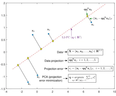
In its standard formulation, PCA approximates data matrixX=[x1,x2, . . . ,xN] ∈ RD×N by another low-rank matrix product QST, where Q ∈ _RD×K, S ∈ _RN×K and K < d = rank(X), so that the squared L2-norm of the approximation error is minimized. That is, standard PCA is formulated as [16]

(QL2,SL2)= argmin

Q∈_RD×K_,_S_∈

RN×K

kX−QSTk2_F, (1.1)

where the L2-norm (or Frobenius norm) k · k2_F returns the sum of squared entries of its matrix argument. Observing that for any given Q, S = XTQminimizes the error in (1.1),

(15)

we obtain the following formulation QL2= argmin Q∈_RD×K QT_Q₌_I K kX−QQTXk_F2. (1.2)

(1.2) is known as the L2 error minimization problem and can be equivalently rewritten as

QL2= argmin Q∈_RD×K QT_Q₌_I K N Õ i=1 kxi−QQTxik_F2,

where xi = [X]:,i is the i-th sample of X ∈ RD×N. I.e., (1.2) aims at finding theQ that minimizes sum of the squared Frobenius norm error of each entry of the data matrixXand its projection ontoQwhereQ∈_RD×K andQTQ= IK, depicted in Figure 1.1.

We know that the squared Frobenius norm of a matrixM is equal to the trace of the product of the transposed matrix with itself, i.e.,kMk_F2 =tr(MTM), wheretr(·)returns the sum of diagonal entries of its matrix argument. Therefore, (1.2) can be expanded as

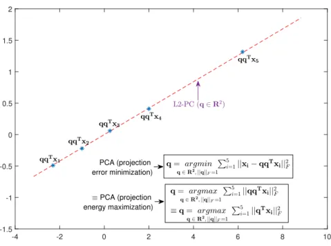
QL2= argmin Q∈RD×K QTQ=IK kX−QQTXk_F2 = argmin Q∈RD×K QTQ=IK tr(X−QQTX)T(X−QQTX) = argmin Q∈RD×K QTQ=IK kXk2_F − kQTXk_F2 =argmax Q∈_RD×K QT_Q₌_I K kQTXk2_F

That is,QL2can equivalently be found by the projection maximization

QL2 =argmax Q∈_RD×K QT_Q₌_I K QTX 2 F (1.3)

(16)

-4 -2 0 2 4 6 8 10 -1.5 -1 -0.5 0 0.5 1 1.5 2 Data PCA (projection error minimization) Data projection Projection error

Figure 1.1: Projection error minimization PCA.

and, accordingly,SL2 =XTQL2. Again, (1.3) can be rewritten as

QL2=argmax Q∈RD×K QTQ=IK N Õ i=1 QTxi 2 F

. I.e., (1.3) aims at finding the Qthat maximizes the sum of squared Frobenius norm of projection magnitude of each entry of the data matrix XontoQand is depicted in Figure 1.2.

The solution to (1.1), (1.2) and (1.3),QL2, contains theK-dominant left singular-vectors of X, obtained through standard Singular-Value Decomposition (SVD) [17]. Therefore,

(17)

-4 -2 0 2 4 6 8 10 -1.5 -1 -0.5 0 0.5 1 1.5 2 PCA (projection error minimization) PCA (projection energy maximization)

Figure 1.2: Projection variance maximization PCA.

1.2

Outliers

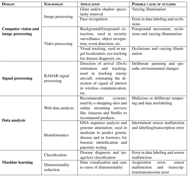
In the big data era, real-world datasets often contain irregular or corrupted measurements that lie far from the nominal data. Such measurements are commonly referred to as “out-liers” [18] and may appear due to various causes such as intermittent sensor malfunctions, errors in data transcription, transmission or labeling, deliberate jamming, or sporadic en-vironmental changes among others. A brief summary of few applications of PCA and possible causes of outliers in various domains is provided in Table 1.1.

Regretfully, standard PCA is known to be very fragile in the presence of outliers, even if they appear in a small fraction of the processed data. The reason is that the L2-norm objec-tive of PCA in (1.3),kQTXk2

F =

ÍN

i=1kQ T_x

(18)

Domain Sub-domain Application Possible cause of outliers

Computer vision and image processing

Image processing

Glare and/or shadow specu-larity removal

Varying illumination

Face recognition Error in data labeling and occlu-sions

Video processing

Background/foreground ex-traction; used in security surveillance, object recogni-tion, event detecrecogni-tion, etc.

Foreground movement, occlu-sions and varying illumination

Visual tracking; used in tar-get localization, eye tracking for disease diagnosis, etc.

Occlusions and varying illumi-nation

Signal processing RADAR signal processing

Direction of arrival (DoA) estimation and tracking; used in tracking enemy aircraft, estimating the di-rection of signal of interest in wireless communication, etc.

Deliberate jamming and spo-radic environmental changes

Data analysis

Web-data analysis

Recommender systems; used by e-shopping sites and online streaming services like Amazon and Netflix to recommend products

Malicious or deliberate tamper-ing and data mislabeltamper-ing

Bioinformatics

DNA sequence analysis and genome annotation; used in medicine to predict genetic disease and in forensics for forensic identification and paternity testing

Intermittent sensor malfunction and labelling/transcription error

Machine learning

Classification Disease diagnosis and im-age/text classification

Error in data labeling and sensor malfunction

Dimensionality reduction

Data visualization and cure to curse of dimensionality

Acquisition error, sensor malfunction and transcrip-tion/transmission error

Table 1.1: Possible causes of outliers in few applications of interest.

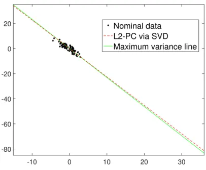
therefore benefiting peripheral, outlying points. A simple line-fitting experiment demon-strates the outlier-sensitivity of L2-PCA in Figure 1.3 and Figure 1.4. In Figure 1.3, there are no outliers and hence the L2 principal-component (L2-PC) is very close to the maxi-mum variance line, however in Figure 1.4, there are 2 outliers among the processed data and therefore the L2-PC deviates away from the maximum variance line (depicting clear attraction towards outlying points). Therefore, the use of traditional PCA in real-world

(19)

-10 0 10 20 30 -80 -60 -40 -20 0 20 _{Nominal data} L2-PC via SVD

Maximum variance line

Figure 1.3: Line-fitting for nominal data.

Figure 1.4: Line-fitting for outlier-corrupted data.

and/or big-data setting where outliers are common leads to unreliable solutions, creating a need for robust PCA.

(20)

The contribution of this thesis are as follows:

• Novel Algorithm for Incremental L1-norm Principal-Component Analysis. • Novel Algorithm for Adaptive L1-norm Principal-Component Analysis.

• Numerical Studies on Outlier-Resistant Signal Subspace Estimation and Tracking. • Experimental Studies on Image Conditioning, Specifically Glare/Shadow Artifacts

Removal from Face Images.

• Experimental Studies on Video Background/Foreground Extraction.

• Experimental Studies on Jammer-Resistant Direction-of-Arrival (DoA) Estimation and Tracking.

(21)

Chapter 2

Background Review

2.1

Robust Principal-Component Analysis

To counteract the impact of outliers in data analysis and processing, researchers have long focused on developing “robust” subspace estimation alternatives. In the popular Robust PCA (RPCA) line of research, the outlier-corrupted dataset is modeled as the summation of a low-rank component that describes the nominal subspace and a sparse component that captures the outliers [19–24]. At first, this RPCA problem formulation suggests a solution where we seek to find the least-ranked low rank component (that best describes the nominal subspace) and the most sparse component to model any outliers amongst processed data. Mathematically, given X = L+ S+n and λ, a constant, where L and S are unknowns, L being the sought-after low rank component,Sbeing the sparse component, andn– the noise in the data matrixX, the RPCA optimization problem can be formulated as

(L,S)=argmin

L,S L+S=X

rank(L)+λ||S||₀, (2.1)

where the zero-norm || · ||₀returns the number of non-zero entries in its matrix argument. (2.1) is a non-convex problem that is NP-hard and no efficient solution exists in literature.

(22)

However, (2.1) can be reformulated as a tractable convex optimization problem by replac-ing the rank with nuclear norn||L||∗and L0-norm by L1-norm, i.e.,

(L,S)=argmin

L,S L+S=X

||L||_∗+λ||S||₁, (2.2)

where nuclear-norm || · ||∗ returns the sum of singular values of its matrix argument and L1-norm || · ||₁ returns the sum of absolute entries of its matrix argument. It was shown in [25] that (2.2) is indeed a convex optimization problem and provided enough conditions to prove the same. Therefore, (2.2) can be solved using convex optimization techniques or algorithms proposed in [19–24]. OnceLandSare successfully extracted, what remains of Xis the noisenand can be neglected.

Another outlier-resistant minimum rank solution is proposed in [26] by solving a con-vex optimization problem, namely nuclear-norm minimization. Authors in [27] propose an efficient rotational invariant L1-norm PCA (R1-PCA) to perform robust PCA. Robust subspace learning (RSL) in [28, 29] proposes algorithms that detect outliers and replace them by neighboring nominal points, or places a weight on each data point to downgrade outliers among the processed data. Fast and low complexity algorithms for robust PCA via gradient descent are proposed in [30].

In another line of research, PCA is robustified by substituting the L2-norm in 1.1 by the L1-norm [31–33]. To date, no exact solution exists for this L1-norm error-minimization PCA, for general K ≥ 1. Another popular approach substitutes the L2-norm by the L1-norm directly on (1.3), effectively removing the squared emphasis that standard PCA places on each datum. This L1-projection-maximizationapproach is also known as L1-PCA, and

(23)

is discussed in the next subsection.

2.2

L1-norm Principal-Component Analysis

L1-PCA [34–36] is another robust approach that performs outlier-resistant PCA and it is mathematically formulated as

QL1= argmax

Q∈RD×K

QTQ=IK

||QTX||₁, (2.3)

where L1-norm k · k₁returns the sum of absolute entries of its matrix argument. Contrary to what is true for standard PCA in (1.1)-(1.3), projection-maximization PCA and L1-error-minimization PCA are not equivalent. Moreover, it has been shown [34] that the K L1-PCs in (2.3) have to be jointly computed.

In [36], Kwak proposed an early approximate solver for (2.3) with complexityO(N2DK). The solver of [36] first approximates the dominant L1-PC (K = 1) of X and then com-putes the remaining K−1 L1-PCs through a sequence of deflating null-space projections. In [37], Nie et al. targeted the problem of computing jointly allK ≥ 1 L1-PCs ofXand, for this task, they proposed a “non-greedy” alternating-optimization algorithm of complexity O(N2DK +N K3). A semi-definite programming (SDP) approach for (2.3) was proposed by McCoy and Tropp in [38] with cost O(K N3.5log(1/) + K L(N2 + DN)) for desired accuracy . Authors in [39] presented a low-cost/high-performance L1-PCA/SVD hybrid model.

The exact solution to L1-PCA was delivered for the first time in [34] where authors reformulated (2.3) as an equivalent combinatorial optimization problem over N K {±1}

(24)

variables. The algorithms of [34] solve (2.3) exactly with complexity O(2N K), in general, orO(NdK−K+1)whend= rank(X)is a constant with respect toN.

2.2.1 Exact Solution

The authors in [34] showed that if

Bopt= argmax

B∈{±1}N×K

||XB||∗, (2.4)

where nuclear norm k · k∗ returns the sum of the singular values of its matrix argument, then L1-PCA in (2.3) is solved by

QL1=Φ(XBopt) (2.5)

where, for any tall matrixA ∈ _Rm×n with SVDA SVD= UΣn×nVT, Φ(A) = UVT. In addition, [34] showed that ||XTQL1||1= ||XBopt||∗and

Bopt= sgn

XTQL1

. (2.6)

Therefore L1-PCA in (2.3) can be cast as an equivalent combinatorial optimization prob-lem over antipodal binary variables in {±1}. The first optimal algorithm in [34] performs exhaustive search over the entire feasibility set of (2.4),{±1}N×K, to obtain a solutionBopt with exponential complexityO(2N K). The second optimal algorithm in [34] first constructs a polynomial-size subset of{±1}N×K,B, wherein a solution to (2.4) is proven to exist, then it searches exhaustively among the elements B to obtainBopt and, through an additional SVD step in (2.5), returns the solution to L1-PCA in (2.3) with overall polynomial cost

(25)

O(NdK−K+1). It is noticeable that the cost of both exact L1-PCA solvers may be imprac-tical in big data applications (large N and/or d), and thus there was a need for algorithms that perform L1-PCA efficiently at lower computation cost while retaining the robustness of L1-norm against outliers.

To this end, Markopoulos et al. in [35] introduced a bit-flipping-based approximate solver for (2.3), labeled L1-BF, with cost O(N Dmin{N,D} + N2(K4+ DK2)+ N DK3), and showed that L1-BF attains very low (if any) performance degradation in the L1-PCA metric, often outperforming its counterparts.

2.2.2 Efficient L1-PCA Through Bit-Flipping (L1-BF)

L1-BF is a state-of-the-art efficient algorithm for L1-PCA based on optimal single bit-flipping iterations [35]. L1-BF has similar cost with standard PCA (i.e., SVD), it exhibits sturdy outlier resistance, and it appears to outperform most of its counterparts in the L1-PCA metric. The incremental and adaptive L1-L1-PCA calculators presented in this work are motivated by L1-BF, which is concisely presented below.

L1-BF commences at some initializationB(0) ∈ {±1}N×K _{(arbitrary or better – a more} intelligent (sv-sign) initialization as shown in [35] for faster convergence) and executes a sequence of optimal single-bit-flipping iterations across which the metric in (2.4) monoton-ically increases. Specifmonoton-ically, at each iteration, L1-BF examines all bits and recognizes the single bit which, when flipped, will offer the highest increase to the metric of (2.4). That is, at thet-th iteration, L1-BF finds

(n,k)=argmax (m,l)∈{1,2,...,N} ×{1,2,...,K} XB(t)−2[B(t)]m,lxme T l,K _∗, (2.7)

(26)

Algorithm L1-BF

Input:X∈_RD×N, init.B∈ {±1}N×K,K ≤rank(X), 1: B←BF(X,B,K) 2: (U,Σ_K×K,V) ←SVD(XB) 3: Q←UVT Output:(Bˆ,Qˆ) ← (B,Q) Function:B←BF(XD×N,B,K) 1: ω←K||X[B]_:_,₁||₂

2: while true (or terminate atN Kiterations)

3: form∈ {1,2, . . . ,N},l∈ {1,2, . . . ,K} 4: am,l ← ||XB−2[B]m,lxmeT_l_,_K||∗ 5: (n,k) ←argmax_m_,_l am,l 6: ifω <an,k 7: [B]_n_,_k ← −[B]_n_,_k, ω←an,k 8: else, break 9: ReturnB

Figure 2.1: Pseudocode of L1-BF algorithm.

where el,K denotes the l-th column of the size-K identity matrix IK and xm is the m-th column of data matrixX. Thereafter, L1-BF flips the(n,k)-th bit ofB(t)setting

B(t+1)=B(t) −2[B(t)]_n_,_ken,NeT_k_,_K. (2.8)

Bit-flipping terminates at iteration t if the nuclear norm in (2.4) cannot further increase by any single-bit flip. Upon termination L1-BF returns ˆB = B(t)as an approximation to Bopt in (2.4) and ˆQ = Φ(XB(t)) as an approximation toQL1 in (2.3), in accordance with (2.5). It was shown in [35] that the bit-flipping iterations converge, since the metric of (2.4) (i) is upper bounded by its exact solution and (ii) increases monotonically across the iterations. Henceforth, for compactness in notation, the L1-BF procedure is summarized as (Qˆ,Bˆ) = L1BF(X;B(0);K). A pseudocode for L1-BF [35] (code available in [40]) is provided in Figure 2.1.

(27)

in [41]. L1-PCA was used for outlier identification and elimination in [42]. It was also used for robust image-fusion, face recognition, and dynamic video foreground/background ex-traction in [43–50]. In [51, 52] L1-PCA was used for DoA estimation. Authors in [53] pro-posed an L1-PCA-based nearest-subspace classifier for radar-based indoor motion recog-nition. L1-PCA-informed reduced-rank filtering for robust interference suppression was presented in [50]. A method for iterative re-weighted L1-PCA was most recently presented in [54]. The exact solution to L1-norm TUCKER-2 decomposition was presented in [55], and an algorithm robust decomposition of 3-way tensors based on L1-norm was proposed in [56].

2.3

Incremental and Adaptive Principal-Component Analysis

Modern big datasets often contain a very large number of measurements (data points), N, of high dimensionality (number of features), D. In such cases, batch-processing all mea-surements inXmay be of prohibitively high computational cost. In some cases, the dataset to be processed is initially unavailable and data points arrive in a streaming fashion and/or the sought-after underlying signal subspace may change over time (e.g., in image/video processing [19, 57–59], dynamic face-ID [60], and DoA estimation/tracking [52, 61]). In-cremental algorithm is used when the underlying signal-subspace is static and an adaptive algorithm is used when the sought after signal-subspace changes over time. Incremental processing algorithms are a subset of adaptive processing algorithms. An adaptive algo-rithm can also be successfully used (as an incremental algoalgo-rithm) in a static subspace con-dition, whereas an incremental algorithm can only be used (as an adaptive algorithm) when the underlying subspace does not change. In streaming data and dynamic signal-subspace

(28)

applications, it is clear that appending every new data point to the previously collected data matrix as a new column and recalculating PCA on the augmented data matrix from scratch leads to unsustainable, continuously increasing complexity. Thus, batch PCA is rather in-appropriate for processing big and/or streaming data. Similarly, the computational cost of batch L1-PCA also becomes prohibitive asN and/orDincrease.

To process big and/or streaming data in an efficient way, researchers have long focused on incremental PCA solutions [62–67]. Thorough revies of incremental PCA algorithms are offered in [57, 68–70]. Similar to the batch solution, incremental PCA calculators per-form well on clean or benign-noise-corrupted data (e.g., data corrupted by zero-mean, small variance additive white Gaussian noise). Conversely, incremental PCA calculators expe-rience significant performance degradation when the processed data include any number of outliers. This observation has motivated extensive documented research on corruption-resistant incremental PCA.

Incremental algorithms inspired by the RPCA [19, 22, 29] problem formulation were proposed in [23, 70–80]. The work in [81] is an online version of robust subspace learn-ing (RSL) in [28]. Online RPCA (OR-PCA) in [73] operates on data arrivlearn-ing sequentially by either accepting or rejecting new data points based on a stochastic model. Grassman-nian robust adaptive subspace tracking algorithm (GRASTA) [82] operates on randomly under-sampled data matrices leading to computational improvements, while accurately tracking the underlying subspace and staying robust against sparse corruptions. The works in [47–49] offer the first incremental L1-PCA algorithms in literature, tailored to perform compressed-sensed domain video surveillance and visual tracking in videos.

(29)

This thesis work presents a complete algorithmic framework for both incremental and adaptive L1-PCA. The first algorithm computes L1-PCA incrementally, processing one measurement at a time, with low computational and memory requirements. The second al-gorithm revises the computed L1-PCA as new measurements arrive, demonstrating both ro-bustness against outliers and adaptivity to signal-subspace changes and thus is appropriate for subspace-tracking applications. The proposed algorithms are evaluated in an array of experimental studies on subspace estimation, video surveillance (foreground/background separation), image conditioning, and direction-of-arrival (DoA) estimation. The sequel provides a comprehensive explanation along with pseudocodes for the proposed incremen-tal and adaptive L1-PCA algorithms.

(30)

Chapter 3

Proposed Algorithms

3.1

Proposed Algorithm for Incremental L1-PCA (L1-IPCA)

The proposed algorithm calculates incrementally theKL1-PCs of data matrixX= [x1,x2, . . . ,xN] ∈ RD×N as its columns arrive in a streaming fashion. In the case that all columns ofX are

available beforehand, the proposed algorithm processes them one-by-one for complexity savings.

To initialize, we first collect a small batch ofndata points fromX, say Y0 = [X]:,1:n ∈ RD×n with rank(Y0) ≥ K. Then, we run L1-BF iterations onY0, with some initialization B ∈ {±1}n×K, to obtain the first approximate L1-PCA solution(Qˆ0,Bˆ0)=L1BF(Y0;B;K). When a new data pointx_i(in) = [X]_:_,n+iarrives,i= 1,2, . . . ,N−n, we first pass it through an L1-PC-informed reliability check. Specifically, similarly to [43], the L1-reliabilityof x(_iin) is defined as its angular proximity to the previously calculated L1-PCs ˆQi−1,

r x(_iin); ˆQi−1 = Qˆ T i−1x (in) i 2 2 x (in) i 2 2 . (3.1)

Based on the outlier resistance of L1-PCA, (3.1) constitutes a measure for determining weatherx_i(in) is clean (i.e., close to the nominal data subspace), or outlying/corrupted.

(31)

set close to 1), thenx(_iin) is disregarded as a possible outlier and we maintain the previous L1-PCA solution (Qî,Bî) = (Qî−1,Bî−1)and the previous memory batchYi = Yi−1. If, on the other hand,r(x(_iin); ˆQi−1)> τ, thenx(in)i passes the reliability check and it is admitted for processing; thei-th L1-PCA update(Qî,Bî)is computed as follows. First,x(in)_i is appended toYi−1, forming the augmented memory batch

˜ Yi−1= h Yi−1, x(in)i i ∈_RD×(n+1). (3.2)

Then, motivated by the optimality condition in (2.6), we compute

˜ Bi−1= sgn ˜ YT_i₋₁Qˆi−1 ∈ {±1}(n+1)×K, (3.3)

and use it as initialization for L1-BF iterations on ˜Yi−1. At the end of the L1-BF iterations, we obtain ˆ Bi, Qˆi =L1BF ˜ Yi−1; ˆBi−1;K . (3.4)

We notice that the number of data points in memory increased fromninYi−1ton+1 in ˜Yi. In order to maintain limited storage and computational cost, we proceed with discarding one of the points in ˜Yi−1. Specifically, similar to [48], we discard the point with the mini-mum L1-reliability (i.e., the least angular proximity to the newly updated L1-PC subspace) as defined in (3.1). Formally, L1-IPCA identifies

jmin = argmin j=1,2,...,n+1 r _˜ Yi−1 :,j; ˆQi , (3.5)

(32)

Proposed Algorithm L1-IPCA Input:Y,K,τ 1: B←arbitrary 2: (B,Q) ←L1BF(Y,B,K) 3: Whenxarrives, 4: (B,Q,Y) ←uL1BF(Y,x,Q,K, τ) Output:(_Bˆ_,_Qˆ) ← (B,Q) Function:(B,Q,Y, τ) ←uL1BF(Y,x,Q,K, τ) 1: r←L1rel(x,Q) 2: ifr> τ 3: Y˜ ← [Y,x] 4: B←sgn(Y˜TQ) 5: (B,Q) ←L1BF(Y˜,B,K) 6: rj←L1rel([Y˜]:,j,Q),j=1, . . . ,n+1 7: j_min←argmin_j₌₁_,...,_n₊₁rj 8: Y← [_Y˜]_:_,_{₁_,...,_n₊₁_}\_j min 9: ReturnB, Q, Y Function:r←L1rel(x,Q) 1: r← | |Q T_x_{| |}2 2 | |x| |2 2 2: Returnr

Figure 3.1: Pseudocode of proposed L1-IPCA algorithm.

and discards the(jmin)-th column of ˜Yi−1, setting thei-th memory matrix

Yi = _˜ Yi−1 :,{1,...,n+1}\jmin ∈R D×n_. (3.6)

In view of the above, the proposed algorithm has multiple lines of defense against out-liers. First, L1-IPCA starts with calculating the L1-PCs of a small original batch. These L1-PCs, being robust against any outliers in the original batch, set a first measure of reli-ability for future processed points. Then, the relireli-ability of an incoming point is evaluated by means of the previously computed L1-PCs, thus protecting the incremental L1-PCA procedure against processing outliers. Finally, any point that passes the reliability check is processed by the robust L1-BF procedure. A detailed description of the proposed L1-IPCA is provided in Figure 3.1.

(33)

Complexity. According to [35], L1-BF returns theK (approximate) L1-PCs of ˜Yi ∈ RD×nwith costO(nDmin{n,D}+n2K2(K2+min{n,D})), for anyi. Sinceitakes values 1,2, . . . ,N−n, the total cost of L1-IPCA isO(NnDmin{n,D}+Nn2K2(K2+min{n,D})), linear in N. That is, if n > D, then the cost isO(Nn2K2(K2+D)); on the other hand, if

D ≥ n, the cost isO(Nn2(K4+K2n+D)).

Comparison with [48].At this point, it is worth noting that the pioneering work in [48]

also proposed L1-BF updates for incremental L1-PCA in compressed-sensed-domain video surveillance. The proposed L1-IPCA algorithm differs from the one in [48] in three main ways. First, instead of (3.3), the algorithm of [48] sets the L1-BF-initialization matrix to

˜ Bi = _ˆ BT_i₋₁,bexact T_, (3.7) where bexact= argmax b∈{±1}K Y˜i−1 _ˆ BT_i₋₁,bexact T _∗. (3.8)

To identify bexact, [48] first finds ˜Yi−1BˆT_i−1 with cost O(KnD); then, for each of the 2 K

candidate solutions in {±1}K_{, it performs an SVD of a} _D _×_K _{matrix. Thus, initializing} L1-BF as in [48] costs O(KnD + 2KDK2). The proposed initialization in (3.3) attains similar performance and costs onlyO(KnD). Secondly, the memory-batch size-preserving step removes the entry of the memory batch that lies farthest from the current L1-PCs by identifying

jmin =argmin 1≤j≤n

||yj−QˆQˆTyj||2F, (3.9)

(34)

i-th memory matrixYi =

_˜ Yi−1

:,{1,...,n}\jmin ∈R

D×n_{before PC-update. However, L1-IPCA}

discards the entry of ˜Yi−1with the least L1-reliability value to obtain ˜Yi after PC-update. A third important difference is that the proposed algorithm updates the L1-PCA solution only on incoming points that pass the L1-PC-informed reliability check ( [48] processes every incoming point). Thus, L1-IPCA has an additional line of defense against outliers in the processed data.

(35)

3.2

Proposed Algorithm for Adaptive L1-PCA (L1-APCA)

L1-IPCA presented above is tailored to cases that the sought-after signal subspace is con-stant across all processed data. In many signal processing applications however it is desired to track a dynamic signal subspace that changes across the collected data points (e.g., in direction-of-arrival tracking). To this end, an algorithm for adaptive L1-PCA (L1-APCA), derived by two main modifications of L1-IPCA is proposed as follows.

3.2.1 Modification 1: Reliability Threshold Adjustment

When the signal subspace changes significantly, new incoming points may fail the reliabil-ity check and be inserted to the secondary memory or discarded. Assuming that outliers appear rather sporadically, when multiple incoming points fail the reliability check one af-ter the other, then this is a strong indication that the signal subspace has changed. Thus, in L1-APCA we consider adjustable reliability threshold that decreases every time an incom-ing point fails the reliability check and resets whenever an incomincom-ing point is admitted for processing.

Specifically, let thresholdτi denote the reliability threshold by which thei-th incoming pointx(in)_i is evaluated, with initialization τ1 = τ. Ifr

x_i(in); ˆQi−1

< τi andx_i(in) fails the reliability check, then we reduce τi+1 = τiρ, for some predetermined decrease ratio ρin (0,1]. Clearly,ρ= 1 corresponds to fixed threshold, as used in L1-IPCA. Ifx(in)_i passes the reliability check, thenτi+1is reset toτ.

(36)

3.2.2 Modification 2: Preserve Recent Measurements

Consider a significant change of the nominal signal subspace. Consider also that an in-coming pointx(in)_i from the new signal subspace passes the reliability check (possibly after threshold reduction) and is inserted in ˜Yi−1. x_i(in) will contribute to an update of the PCs from ˆQi−1 to ˆQi. However, if most of the points in ˜Yi−1 are drawn from the previous/old signal subspace, then the new PCs in ˆQi may remain almost invariant. Thus, when the reli-ability of points in memory ˜Yi−1is evaluated by means of ˆQias in (3.5),x_i(in)may be found to be the least coherent point and as such be discarded from ˜Yi−1. Most certainly, such an event would inhibit the subspace tracking process. Therefore, in L1-APCA, we revise steps in (3.5)-(3.6) so that the q < n most recently added measurements are not dropped from

˜

Yi−1. That is, thei-th memory matrix is defined asYi =

_˜ Yi−1 :,{1,...,n+1}\j_min ∈R D×n_where jmin = argmin j=1,2,...,n+1−q r Y˜i−1 :,j; ˆQi . (3.10)

A detailed description of L1-APCA, including all above modifications, is provided in the pseudocode of Figure 3.2.

(37)

Proposed Algorithm L1-APCA Input:Y,K,q,τmax,ρ 1: B←arbitrary, τ←τ_max 2: (B,Q) ←L1BF(Y,B,K) 3: Whenxarrives, 4: (B,Q,Y, τ) ←aL1BF(Y,x,Q,K,q, τmax, τ, ρ) Output:(Bˆ,Qˆ) ← (B,Q)

Function:(B,Q,Y,S, τ) ←aL1BF(Y,x,S,Q,K,m,q, τmax, τ, ρ) 1: r←L1rel(x,Q) 2: ifr> τ 3: Y˜ ← [Y,x],τ←τ_max 4: B←sgn(_Y˜T_Q₎ 5: (B,Q) ←L1BF(_Y˜_,_B_,_K) 6: rj←L1rel([Y˜]:,j,Q), j=1, . . . ,n+1 7: jmin←argminj=1,...,n+1−qrj 8: Y← [Y˜]_:_,_{₁_,...,_n₊₁_}\_j min 9: else 10: τ←τρ 11: ReturnB, Q, Y, τ Function:r←L1rel(x,Q) 1: r← | |Q T_x_{| |}2 2 | |x| |2 2 2: Returnr

(38)

Chapter 4

Numerical and Experimental Studies

4.1

Synthetic Data Analysis

4.1.1 Toy Example – Line-Fitting

The performance of the proposed L1-IPCA algorithm is first evaluated with a line-fitting experiment. Considerz ∈ _R(D=2)×(K=1), with kzk₂ = 1 and α = 10. N = 100 data points are drawn fromN (02, αzzT)to form matrixX ∈R2×100. Every entry ofXis corrupted with zero-mean additive white Gaussian noise (AWGN) of variance 1 fromN (0,1); this results in rank(X) = D = 2. To approximatez, L1-IPCA is run onXforK = 1, setting memory batch-sizen=10 and L1-reliability thresholdτ =0.85. In Figure 4.1(a), the nominal data points (black asterisks) and the L1-PC obtained by L1-IPCA after processing all N points are plotted. In the same figure, the lines obtained by SVD, incremental singular-value-decomposition (ISVD) [62], and GRASTA [82] are plotted. It is observed that all methods perform similarly, approximating well the line defined byz(maximum-variance line).

Then, columns 5, 57 and 74 of X are corrupted by adding to them corruption from N (02, βppT), where β = 40α andp ∈R2×1 is such that||p||2 = 1 and arccos(pTz)= 78◦. L1-IPCA is run again on XforK = 1, keepingn= 10 andτ = 0.85. In Figure 4.1(b), the L1-PC obtained by L1-IPCA after processing all N data points is plotted. In addition, the

(39)

-15 -10 -5 0 5 10 15 20 25 30 35 -100 -80 -60 -40 -20 0 20 40 Nominal data Maximum-variance line SVD ISVD GRASTA L1-IPCA (proposed) (a) -15 -10 -5 0 5 10 15 20 25 30 35 -100 -80 -60 -40 -20 0 20 40 Nominal data Outliers Maximum-variance line SVD ISVD GRASTA L1-IPCA (proposed) (b)

Figure 4.1: Line-fitting experiment. PC calculation on (a) clean/nominal and (b) outlier-corrupted data;

(40)

lines obtained by SVD, ISVD [62], and GRASTA [82] are also plotted. This time, the L2-norm based methods (SVD, ISVD) are significantly misled by the corrupted/outlying data. GRASTA [82] displays some deviation. Interestingly, the proposed L1-IPCA algorithm remains almost unaffected by the outliers and very close to the maximum-variance line of z.

4.1.2 Incremental subspapce estimation with L1-IPCA

Next, the performance of L1-IPCA in intermediate incremental updates is evaluated. Specif-ically, the normalized subspace error of ˆqi (i.e., the approximate L1-PC after x(in)_i is pro-cessed) is measured as ei= 1 2||zz T ₋ _ˆ qiqˆTi || 2 _{∈ [} 0,1]. (4.1)

In this experiment, D = 5 and N = 200 points are drawn from the nominal distribution N (05, αzzT), for α = 55, ||z||2 = 1, to form data matrix X ∈ R5×200. All entries of X are also corrupted by AWGN from N (0,1). Columns 7, 60, 125 and 170 of X are also corrupted additively by outliers from N (05, βppT)where β = 30α, p ∈ R5×1, ||p||2 = 1, and arccos(pTz) = 74.33◦. Setting n = 20, K = 1, and τ = 0.66, the proposed L1-IPCA algorithm is run while evaluating ei for everyi. The average value of {ei}_iN₌−n

1 over 2000 independent realizations of nominal data points, noise, and outlier corruption is calculated. In Figure 4.2, ei vs. update indexi is plotted. Together with the proposed algorithm, the performance of standard PCA (SVD), batch-calculated jointly on[X]_:_,_1:_i₊_n (i.e., for index

i, we carry out SVD on entire [X]_:_,_1:i+n), L1-BF [50], also batch-calculated on [X]:,1:i+n,

(41)

0 20 40 60 80 100 120 140 160 180

Update index

i

0 0.05 0.1 0.15 0.2 0.25 0.3 0.35 0.4

Average normalized subspace error

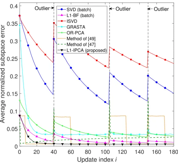
SVD (batch) L1-BF (batch) ISVD GRASTA OR-PCA Method of [49] Method of [47] L1-IPCA (proposed) Outlier Outlier Outlier

Figure 4.2: Subspace estimation experiment. Average normalized subspace error versus update index i;

D=5,N =200,K =1;n=20,τ=0.66.

are also plotted1.

Clearly ISVD [62] and SVD start at a relatively high normalized error due to the pres-ence of one outlier-corrupted point in [X]_:_,_1:(n=20) (point [X:,7]). These methods exhibit improvement as they process nominal points. However, when they encounter another out-lier[X:,60], [X:,125]and[X:,170](dashed vertical line), they deviate again from the nominal

1_{Open access MATLAB codes were found in the GitHub library [84]; the MATLAB implementation of ReProCS [72] was available}

(42)

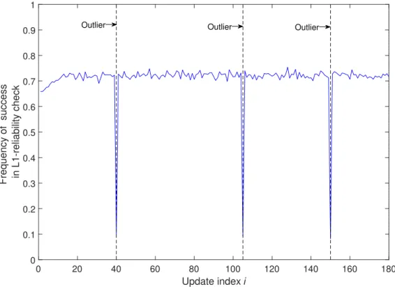
subspace. GRASTA subspace error starts at 0.3 and drops to 0.035, quickly reaching lower error and remains at this level throughout the remaining updates, almost unaffected by the outliers. L1-BF, the method of [49] and the method of [47] start at an error of about 0.08 and OR-PCA starts at an error close to 0.12. The method of [47] quickly drops to a lower error because it finds the exact bit-flipping vector,bexact, when a new point arrives, through exhaustive search. L1-BF and OR-PCA drop towards lower error but show some respon-siveness to outliers. The method of [49] and the method of [47] also respond to outliers. The method of [49] drops to low error after processing n = 20 nominal points since it encountered an outlier and the method of [47] drops to low error very quickly after pro-cessing 1 nominal point since it encountered an outlier. It is observed that the average error of the method of [47] monotonically increases throughout all updates, owing to the memory-batch size-preserving step (3.9). The proposed L1-IPCA algorithm starts from an error of 0.08 due its initialization to the L1-PC of[X]_:_,_1:₍_n₌₂₀₎ (obtained by L1-BF). During the incremental updates, the proposed algorithm converges fast to very low subspace error (close to 0) and remains there throughout all the updates, staying practically unaffected by the outlier-corrupted points inX, thus outperforming every counterpart throughout all up-dates. With its L1-reliability check feature, L1-IPCA strives to avoid processing outliers. For the same experiment described above, the frequency with which [X]_;,i,i =n+1, . . . ,N, passes the reliability check is plotted in Figure 4.3. Noticeably, for τ = 0.66 all nominal points pass the L1-reliability check more that 70% of the time and is admitted for process-ing. On the other hand, L1-IPCA manages to detect and discard the outliers[X:,60],[X:,125] and[X:,170]more than 90% of the time.

(43)

0 20 40 60 80 100 120 140 160 180 Update index _i 0 0.1 0.2 0.3 0.4 0.5 0.6 0.7 0.8 0.9 1

Frequency of success in L1-reliability check

Outlier Outlier Outlier

Figure 4.3: Subspace estimation experiment. Frequency of success versus update indexi.

20 40 60 80 100 120 140 160 180 Update index i 0 1 2 3 4 5 6 7 8 9 Average time (s) 10-4 SVD (batch) L1-BF (batch) ISVD GRASTA OR-PCA Method of [49] Method of [47] L1-IPCA (proposed) 146 148 150 152 154 5 10 15 10-5

Outlier Outlier Outlier

(44)

Next, for the same study and same algorithms, the average computation time a each up-date step is plotted in Figure 4.42. Clearly L1-BF (batch processing) has a higher compu-tational cost, expectedly increasing acrossi; interestingly, when L1-BF processes outliers, its computation effort increases as more bit-flipping iterations are needed for convergence. Batch SVD has lower cost, also monotonically increasing withi. All incremental methods need very low average computation time below 155µs, for every i. Interestingly, the cost of L1-IPCA drops to 10µs fori = 60−n,i = 125−nandi = 170−n, since 90% of the time[X]_:_,₆₀,[X]_:_,₁₂₅and[X]_:_,₁₇₀are not admitted for processing.

2_{Reported computation times are measured in MATLAB R2017a, run on a computer equipped with Intel(R) core(TM) i7-6700}

(45)

4.1.3 Subspace tracking with L1-APCA

Next, we evaluate the performance of the proposed adaptive L1-PCA algorithm (L1-APCA) for subspace tracking. We consider data matrixX ∈_R5×250, the first 130 columns of which are drawn fromN (05, αzzT), where||z||2 = 1 andαis the same as in the study of Figure 4.2. The last 120 columns are drawn from N (05, αz0z0T), wherez0 ∈ R5×1, kz0k2 = 1 and arccos(z0Tz) = 32.43◦. That is, the nominal subspace changes after the 130 first points are processed. All entries of X are corrupted by AWGN from N (0,1). Columns 7, 60 and 210 of X are once again corrupted additively by outliers from N (05, βppT), where ||p||₂ = 1 and β is the same as in the previous experiment. arccos(pTz) = 84.26◦ and arccos(pTz0) = 77.53◦. We set L1-APCA parametersn = 20, τ = 0.8, threshold decrease ratio ρ = 0.5, and number of maintained recent pointsq = 0.75n (i.e., at each adaptation instance, we preserve in the memory matrix 75% of the points processed most recently). In Figure 4.5 we plot the normalized subspace error calculated as ei = 1₂||zzT −qˆiqˆT_i ||2for i ≤ 130 andei = 1₂||z0z0T −qˆiqˆT_i ||2fori > 130. Together with L1-APCA, we plot the per-formance of SVD (batch), L1-BF (batch), ISVD, GRASTA, and OR-PCA. Noticeably the L2-norm based methods deviate from the nominal subspace when they process outliers and display slower response to subspace changes. GRASTA, OR-PCA and L1-BF are relatively robust against outliers compared to the L2-norm based methods. L1-APCA outperforms all counterparts, exhibiting fast convergence to the first nominal subspace (z), sturdy outlier resistance, and fast adaptation to the second nominal subspacez0. GRASTA adapts slightly faster than L1-APCA to the subspace change, converging though to higher subspace error. In Figure 4.7, the frequency of success of [X]_:_,i,i = n+1, . . . ,N in the reliability check is

(46)

20 40 60 80 100 120 140 160 180 200 220 Adaptation index i 0 0.1 0.2 0.3 0.4 0.5 0.6

Average normalized subspace error

SVD (batch) L1-BF (batch) ISVD GRASTA OR-PCA L1-APCA (proposed)

Outlier Subspace _Outlier

change

Figure 4.5: Subspace tracking experiment. Average normalized subspace error versus adaptation index i;

D=5,N =250,K =1;n=20,τmax =0.8,ρ=0.35 andq=0.75n; Subspace change after 130−npoints.

0 50 100 150 200 Adaptation index i 0 0.1 0.2 0.3 0.4 0.5 0.6 0.7 0.8 0.9 1 Average Outlier Subspace change Outlier

(47)

plotted. This plot is best interpreted together with Figure 4.6, where the average value of τi versusi is plotted. Clearly, for increased maximum threshold τmax = 0.8, most nomi-nal points are tested with threshold close to 0.6 and exhibit frequency of success (i.e., any point being able to participate in PC-adaptation) close to 0.65. Once again, both outliers are identified and discarded more than 90% of the time. When an outlier is discarded,τiis decreased to 35% of τmax. Expectedly, the first few points points from the new subspace are often discarded; though, dropping the threshold with reduction factor ρ = 0.35 allows for quick adaptation.

In Figure 4.8, the average update time for each algorithm versus i is plotted. Once again, L1-BF is the most computationally expensive algorithm and its cost increases when it processes outliers. On the other hand, all incremental methods update on average in less than 0.2ms and again, L1-reliability success rates affect the execution time of the proposed L1-APCA algorithm (similar to Figure 4.4).

(48)

0 50 100 150 200 Adaptation index i 0 0.1 0.2 0.3 0.4 0.5 0.6 0.7 0.8 0.9 1

Frequency of success in L1-reliability check

Outlier Subspace Outlier

change

Figure 4.7: Subspace tracking experiment. Frequency of success versus adaptation indexi.

20 40 60 80 100 120 140 160 180 200 220 Adaptation index i 0 0.2 0.4 0.6 0.8 1 1.2 Average time (s) 10-3 SVD (batch) L1-BF (batch) ISVD GRASTA OR-PCA L1-APCA (proposed) Outlier Subspace change Outlier

(49)

4.2

Image Conditioning

In this experiment, conditioning of face images is performed. An interesting proposition was made by Barsi and Jacobs in [87] stating that images (convex-Lambertian) taken under varying, distant illumination lie near an approximately nine-dimensional (low-dimensional) subspace known as the harmonic-plane. This proposition motivates the glare/shadow ar-tifacts removal experiment wherein we can approximate the image accurately by a low-dimensional subspace. Specifically, we operate on images of a person’s face from the PICS database [88] captured in varying illumination conditions that resulted in unwanted glare and shadow artifacts. 14 images of a single individual captured under varying illumina-tion are chosen and cropped to 200×200 pixels each. Each image is then vectorized and stacked one next to the other as columns of data matrixX∈ _R40000×14_{. In this experiment,} the face characteristics form the sought-after static background whereas the illumination variations (glare and shadow artifacts) constitute foreground outliers that we wish to elimi-nate. We setn= 5 andτ= 0.95 and run the proposed L1-IPCA algorithm to obtainK =5 approximate L1-PCs after processing all 14 images. We remove unwanted illumination artifacts from each vectorized image xi = [X]:,i by projecting it on the span of calculated L1-PCs, ˆQas ˆQQˆTxi. In Figure 4.9 we present (a) an original face instance with glare and shadows, and the same image conditioned by (b) ISVD [62], (c) the method of [64], (d) GRASTA [82], (e) PCP [19], (f) OR-PCA [73, 74], (g) the method of [49], (h) the method of [47] and (i) L1-IPCA (proposed). We observe that ISVD [62] and the method of [64] retain most glare. GRASTA [82], PCP [19], OR-PCA [73, 74], and the method of [49] perform improved glare/shadow elimination. The proposed L1-IPCA algorithm and the

(50)

(a) (b) (c)

(d) (e) (f)

(g) (h) (i)

Figure 4.9: Image conditioning experiment. (a) Original face image with glare and shadows. Image condi-tioned with (b) ISVD [62], (c) the method of [64], (d) GRASTA [82], (e) PCP [19], (f) OR-PCA [73, 74], (g) the method of [49], (h) the method of [47] and (i) L1-IPCA (proposed).

method of [47] demonstrate superior image conditioning.

Next, the experiment is repeated on a different set of face images. 13 images of a diff er-ent face under varying illumination are obtained from the same PICS database. Each image is cropped to 200×200 pixels and vectorized to form the data matrixX ∈ _R40000×13. We

(51)

(a) (b) (c)

(d) (e) (f)

(g) (h) (i)

Figure 4.10: Image conditioning experiment. (a) Original face image with glare and shadows. Image condi-tioned with (b) ISVD [62], (c) the method of [64], (d) GRASTA [82], (e) PCP [19], (f) OR-PCA [73, 74], (g) the method of [49], (h) the method of [47] and (i) L1-IPCA (proposed).

re-run the experment by setting n = K = 4 and τ = 0.975. In Figure 4.10 we present (a) an original face instance with glare and shadows, and the same image conditioned by (b) ISVD [62], (c) the method of [64], (d) GRASTA [82], (e) PCP [19], (f) OR-PCA [73, 74], (g) the method of [49], (h) the method of [47] and (i) L1-IPCA (proposed). We observe

(52)

ISVD Method of [64] GRASTA PCP OR-PCA Method of [49]Method of [47] L1-IPCA (proposed) 0 0.01 0.02 0.03 0.04 0.05 0.06 0.07 0.08 0.09 Time consumed (s) Male face (N=13, K=4) Female face (N=14, K=5)

Figure 4.11: Time consumed for image conditioning

similar performance compared to the previous case, i.e, ISVD [62] and the method of [64] retain most glare. PCP [19], OR-PCA [73, 74] perform improved glare/shadow elimina-tion. GRASTA [82], the method of [49], the method of [47] and the proposed L1-IPCA algorithm demonstrate superior image conditioning.

The time required by each method to compute the underlying subspace ˆQ(onto which each image is projected for glare removal) is computed and plotted as a bar-graph in Figure 4.11. It is observed that, for processing the male face (K = 4; see blue bars), method of [64], method of [47], method of [49], ISVD consume similarly higher time, followed by PCP with lower time consumed. GRASTA and OR-PCA consume even lower time whereas the proposed L1-IPCA algorithm consumes the least time. For processing the female face

(53)

(K = 5; see yellow bars), each method consumes proportionally higher time. However the proposed L1-IPCA algorithm displays strikingly fast performance across the board. Therefore, the image conditioning experiment concludes that L1-IPCA performs superior glare/shadow artifacts removal at strikingly fast speeds.

(54)

4.3

Background

/

Foreground Separation in Video Sequences

Video foreground extraction is an important computer vision application used, e.g., in real-time gesture/object identification, human-computer interaction, security surveillance, traf-fic monitoring, and optical-motion capture [89, 90]. The background of each frame forms the static nominal subspace while moving foreground components (e.g., people and vehi-cles) constitute intermittent outliers. The foreground components of the video sequence are typically extracted by first estimating the underlying background of the video and then subtracting it from the original frame. For this experiment, we use a surveillance video recorded at a shopping center in Portugal, available in the standard CAVIAR database [91]. The video consists of N = 474 frames of size 202 by 269 pixels. Video processing is carried out as follows. We cut the video so that last 3 frames in Y(0) contain foreground movement (man), vectorize each video frame and arrange them as columns of data matrix X ∈ _R54338×474. We set n = 20 andτ = 0.9 and apply L1-IPCA to compute theK = 5 L1-PCs of the video sequence ˆQ∈_R54338×5. The background of thei-th framexi = [X]:,iis obtained by projecting it onto the computedK L1-PCs asx(back)_i = QˆQˆTxi. Then, the fore-ground frame is obtained through backfore-ground subtraction; that is x(fore)_i = xi −x_i(back). In Figure4.12a, we present the 135-th frame of the processed video sequence. In addition, in Figure 4.12 we present the background extracted by (b) ISVD [62], (c) GRASTA [82], (d) PCP [19], (e) Online-RPCA via stochiastic optimization (OR-PCA) [74], (f) RPCA [29], (g) ReProCS [72], and (h) L1-IPCA (proposed). Foreground extracted by (i) ISVD [62], (j) GRASTA [82], (k) PCP [19], (l) OR-PCA [74], (m) RPCA [29], (n) ReProCS [72], and (o) L1-IPCA (proposed). We observe that background computed by ISVD [62] exhibits a

(55)

(a) (b) (c) (d)

(e) (f) (g) (h)

(i) (j) (k) (l)

(m) (n) (o) (p)

(q)

Figure 4.12: Video processing experiment – video 1. (a) Original frame. Background extracted by (b) ISVD [62], (c) GRASTA [82], (d) PCP [19], (e) OR-PCA [74], (f) RPCA [29], (g) ReProCS [72], (h) method of [47], and (i) L1-IPCA (proposed). Foreground extracted by (j) ISVD [62], (k) GRASTA [82], (l) PCP [19], (m) OR-PCA [74], (n) RPCA [29], (o) ReProCS [72], (p) method of [47], and (q) L1-IPCA (proposed).

(56)

non-negligible “ghostly” appearance of the walking man, whose blurred/inaccurate figure also appears in the foreground. GRASTA [82], PCP [19], and RPCA [29] exhibit similar performance with the smudged appearance of the man in the computed background. OR-PCA [74] performs clearly better than the previous methods. The method of [47] extracts a clean background but "ghostly" appearances of the ladies in the last frame are seen on the extracted foreground. The proposed L1-IPCA algorithm, together with ReProCS [72], demonstrate similarly high performance, obtaining the clean background and a foreground with a well defined outline of the man, together with his shadow.

Next, we obtain a surveillance video of the entrance lobby at INRIA labs in France from the same CAVIAR database [91]. We keep only the first N = 295 frames, vectorize them, and arrange them as columns of data matrix X ∈ _R54338×295. We set n = 14 and τ = 0.9 and repeat the experiment to obtain the background and foreground of the 80-th frame of the video usingK =3 PCs. In Figure 4.13, we plot the performance of ISVD [62], GRASTA [82], PCP [19], OR-PCA [74], RPCA [29] and ReProCS [72] (background and extracted foreground). We observe that ISVD [62], GRASTA [82], PCP [19], and RPCA [29] demonstrate again similar performance as before –i.e., ghostly appearance of the man in the extracted background and his blurred figure in the foreground. The method of [47] extracts a clean background but "ghostly" appearances of the foreground movement in the last frame is seen on the extracted foreground. On the other hand, OR-PCA [74], ReProCS [72], and L1-IPCA obtain similarly clean background and well-defined foreground.

Finally, we operate on the “Curtain Video” [85]. We collect N = 103 frames of size 45 by 46 pixels, vectorize them, and arrange them as columns of data matrix X ∈ _R2520×103.

(57)

(a) (b) (c) (d)

(e) (f) (g) (h)

(i) (j) (k) (l)

(m) (n) (o) (p)

(q)

(58)

We setn = 5 andτ = 0.999 and repeat the above experiment, forK = 2. In Figure 4.14, we present the foreground and background of the 50-th frame as obtained by ISVD [62], GRASTA [82], PCP [19], OR-PCA [74], RPCA [29], and ReProCS [72]. We notice that this experiment poses some particular challenges: the man’s shirt matches the background curtain color, the man (foreground) is stationary in many frames, and the curtain in the background of this video moves continuously leading to slow background changes. In Figure 4.14, we observe that the background frames obtained by ISVD [62], GRASTA [82], PCP [19], OR-PCA [74], and RPCA [29] retain the majority of the foreground (man); at the same time, the corresponding foreground frames do not capture the man clearly. the method of [47] has slight reminiscence of the man in the foreground and traces of the moving (background) curtain in its extracted foreground. On the other hand, ReProCS [72] obtains a cleaner background with slight presence of the man, while the proposed L1-IPCA algorithm obtains an entirely clean background. The foreground extracted by L1-IPCA contains some traces of the moving (background) curtain, which are not present in the foreground of ReProCS [72].

4.4

Direction-of-Arrival Estimation and Tracking

Going forward, an experiment on direction-of-arrival (DoA) estimation and tracking is performed. We consider uniform linear antenna array (ULA) of D = 4 antenna elements that capture N = 70 snapshots of an incoming signal of interest that arrives from angle φ = −40◦ with respect to the broadside. The i-th down-converted and pulse-matched

(59)

snapshot takes the form

xi = bis(φ)+ni, i= 1,2, . . . ,70 (4.2)

wheres(φ) =[1,e−jπsin(φ), . . . ,e−jπsin(φ)(D−1)]T is the array-response vector,bi isi-th sym-bol (accounting for transmission energy and channel attenuation) with bi ∈ {±√α}, α = 10, and ni is complex AWGN from CN (04,I4). The 70 snapshots are stacked as the columns of data matrix X = [x1,x2, . . . ,xN] ∈ C4×70. We assume that snapshots 5 and 55 are unexpectedly corrupted by a jamming signal from DoAφo =10◦, carrying a symbol from{±√β}, β= 60.

To estimateφ, the receiver operates as follows. First,Xis realified as ˜X=[<{X},={X}]T ∈ R8×, where<{·} and ={·}return the real and imaginary parts of their arguments respec-tively. Next, we estimate the K = 1 PC of Xby L1-IPCA with parameters n = 20, and τ = 0.9. For approximate L1-PC ˆqi, we compute the L1-PCA-based MUSIC-type [52] spectrum Pi(θ)= 1 k (I8−qˆiqˆT_i)s˜(θ)k2 , (4.3) for θ in Θ = {−π 2, −π 2 + ∆, . . . , π

2 − ∆}, for arbitrarily small step ∆ > 0, and ˜s(θ) =

[<{s(θ)}T,={s(θ)}T]T. Similar to [52], thei-th estimate ofφis given by

ˆ

φi= argmax

θ∈Θ

Pi(θ). (4.4)

We carry out DoA estimation using the PC obtained by batch SVD, ISVD, GRASTA, and OR-PCA. In Figure 4.15, we plot an instance ofP70(θ)for all 5 methods. We observe

(60)

that the L2-based methods SVD and ISVD are misled by the jamming signal and point towardsφo =10◦. On the other hand, the robust GRASTA, OR-PCA, and L1-APCA (most emphatically) point towards the correct DoAφ=−40◦.

Next, by keeping all the parameters the same, we setα= 1 andβ =33 (leading to SNR (source)=0 dB and SNR (jammer)=15dB) and re-run the DoA estimation experiment to plot in Figure 4.16 an instance of P70(θ) for all 5 methods. Again, we observe that SVD and ISVD are misled by the jammer. (they have two peaks, one at the DoA of source and the other at DoA of jammer, however the peak at jammer is higher and hence considered more important). GRASTA, OR-PCA and L1-IPCA point correctly at the source DoA.

In the sequel, we increase N = 200 and steer our focus towards DoA tracking. We consider that in the first 90 snapshots the signal of interest arrives from DoAφ1 =−40◦. In the latter 110 snapshots, the signal of interest arrives from DoAφ2= −35◦(signal subspace change). We consider a jammer atφo=−60◦corrupting snapshots 5, 55, and 135. We run L1-APCA with parameters n=20, τ=0.9, ρ=0.8, andq =0.9nto track the DoA of the signal of interest. In Figure 4.17, we plot the root-mean-squared-error (RMSE) (average over 2000 independent realizations) versus adaptation indexi, calculated as

RMSEi = v u t 1 2000 2000 Õ m=1 |φˆ(_im)−φ|2, _(4.5)

where ˆφ_i(m) is the DoA estimation at thei-th adaptation of the m-th realization. In (4.5), φ = φ1fori ≤ 90 andφ = φ2fori > 90. We observe that SVD and ISVD are mislead by the jammers and attain high RMSE for everyi. GRASTA, OR-PCA, and the proposed L1-APCA exhibit both robustness against jamming and the ability to adapt quickly to changes

(61)

(62)

(a) (b) (c) (d)

(e) (f) (g) (h)

(i) (j) (k) (l)

(m) (n) (o) (p)

(q)

(63)

-80 -60 -40 -20 0 20 40 60 80 0 1 2 3 4 5 6 7 8 9 MUSIC spectrum SVD (batch) ISVD GRASTA OR-PCA L1-IPCA (proposed)

Source DoA Jammer DoA

Figure 4.15: DoA estimation experiment. DoA estimation spectrum P70(θ). N = 70, D = 4, K = 1. φ=−40◦,φo=10◦,α=10,β=60.n=20,τ=0.9. Jamming atx5andx55. -80 -60 -40 -20 0 20 40 60 80 0 0.5 1 1.5 2 2.5 3 MUSIC spectrum SVD (batch) ISVD GRASTA OR-PCA L1-APCA (proposed) Jammer DoA Source DoA

Figure 4.16: DoA estimation experiment. DoA estimation spectrum P70(θ). N = 70, D = 4, K = 1. φ=−40◦,φo=10◦,α=1,β=33.n=20,τ=0.9. Jamming atx5andx55.

(64)

0 20 40 60 80 100 120 140 160 180 Adaptation index _i 0 2 4 6 8 10 12 14 16 18 Average RMSE SVD (batch) ISVD GRASTA OR-PCA L1-APCA (proposed) Jammer Jammer DoA change

Figure 4.17: DoA tracking experiment. RMSE performance versus adaptation indexi. N = 200, D = 4,

K=1. φ1=−40◦,φ2 =−35◦,φo=−60◦,α=10,β=60.n=20,τ=0.9,ρ=0.8,q =0.9n. Jamming at x5,x55, andx135.

(65)

Chapter 5

Quality of Initialization and Parameter Tuning

The quality of initialization memory batch Y0 is important as the reliability of incoming data points is evaluated based on the PCs obtained from Y0. If Y0 is sufficiently outlier-corrupted, the the PCs obtained ˆQ0 might be incorrect and thus new nominal data points will be discarded due to their low reliability with respect to such a ˆQ0. In L1-APCA, because of the threshold decrease ratio ρ and q most recent measurements preserved in memory batch, the algorithm recovers from an incorrect ˆQ0 as it processes new nominal data points. L1-IPCA however, does now have such a mechanism and thus a sufficiently clean memory batch initialization is required.

In the sequel we say a few things about tuning important parameters of our algorithms. In L1-IPCA: the memory batch sizencould be chosen to be sufficiently large such that the ratio of number of nominal points to number of outlier-corrupted points is high (ideally, close to 1). Threshold τ could be chosen close to 1. E.g., in video/image processing experiments we set τto a value close to 1 and obtain good performance. However, if the initial memory batch is not sufficiently clean and/or the noise in the data measurements is high, then a highτwould lead to incorrect solutions. If the confidence of the initial solution

ˆ

(66)

In L1-APCA:n is chosen as in L1-IPCA.τmax could be set close to 1. IfY0 contains many corrupted measurements, the threshold drops due to the use of threshold degradation. The threshold decrease rationρcould be set to a lower value if the expected change in sub-space is drastic and/or if faster adaptation is required during subspace c