Evaluation and metrics framework

econ

stor

Der Open-Access-Publikationsserver der ZBW – Leibniz-Informationszentrum Wirtschaft

The Open Access Publication Server of the ZBW – Leibniz Information Centre for Economics

Nutzungsbedingungen:

Die ZBW räumt Ihnen als Nutzerin/Nutzer das unentgeltliche, räumlich unbeschränkte und zeitlich auf die Dauer des Schutzrechts beschränkte einfache Recht ein, das ausgewählte Werk im Rahmen der unter

→ http://www.econstor.eu/dspace/Nutzungsbedingungen nachzulesenden vollständigen Nutzungsbedingungen zu vervielfältigen, mit denen die Nutzerin/der Nutzer sich durch die erste Nutzung einverstanden erklärt.

Terms of use:

The ZBW grants you, the user, the non-exclusive right to use the selected work free of charge, territorially unrestricted and within the time limit of the term of the property rights according to the terms specified at

→ http://www.econstor.eu/dspace/Nutzungsbedingungen By the first use of the selected work the user agrees and declares to comply with these terms of use.

zbw

Leibniz-Informationszentrum Wirtschaft Leibniz Information Centre for Economics

Catalano, Michele; Giulioni, Gianfranco; Streitberger, Werner; Reinicke, Michael; Eymann, Torsten

Working Paper

Evaluation and metrics framework

Bayreuth reports on information systems management, No. 6

Provided in cooperation with:

Universität Bayreuth

Suggested citation: Catalano, Michele; Giulioni, Gianfranco; Streitberger, Werner; Reinicke, Michael; Eymann, Torsten (2005) : Evaluation and metrics framework, Bayreuth reports on information systems management, No. 6, urn:nbn:de:bvb:703-opus-3629 , http:// hdl.handle.net/10419/52625

Bayreuther Arbeitspapiere zur Wirtschaftsinformatik

Lehrstuhl für

Wirtschaftsinformatik Information Systems Management

Bayreuth Reports on Information Systems Management

No. 6

2005

Michel Catalano, Gianfranco Giulioni (Universita delle Marche Ancona), Werner Streitberger, Michael Reinicke, Torsten Eymann (University of Bayreuth)

Evaluation and Metrics Framework

vorläufiger Ergebnisse, die i. d. R. noch für spätere Veröffentlichungen überarbeitet werden. Die Autoren sind deshalb für kritische Hinweise dankbar.

which will usually be revised for subsequent publications. Critical comments would be appreciated by the authors.

Alle Rechte vorbehalten. Insbesondere die der Übersetzung, des Nachdruckes, des Vortrags, der Entnahme von Abbildungen und Tabellen – auch bei nur auszugsweiser Verwertung.

All rights reserved. No part of this report may be reproduced by any means, or translated.

Authors: Information Systems and Management Working Paper Series

Edited by:

Prof. Dr. Torsten Eymann

Managing Assistant and Contact:

Raimund Matros Universität Bayreuth

Lehrstuhl für Wirtschaftsinformatik (BWL VII) Prof. Dr. Torsten Eymann

Universitätsstrasse 30 95447 Bayreuth Germany

Email: [email protected] ISSN

Michele Catalano, Gianfranco Giulioni (Universitá delle Marche Ancona), Werner Streitberger, Michael Reinicke, Torsten Eymann (University of Bayreuth)

IST-FP6-003769 CATNETS

Work Package 4 Deliverable T0+12

Evaluation and Metrics Framework

Contractual Date of Delivery to the CEC:31.08.2005 Actual Date of Delivery to the CEC:31.08.2005

Author(s):Michele Catalano, Gianfranco Giulioni, Werner Streitberger, Michael Reinicke, Torsten Eymann

Workpackage:WP 4 Est. person months:20 Security:public

Nature:T0+12 Deliverable Version:1

Total number of pages:40 Abstract:

In this work package we build a framework to evaluate different scenarios in the CATNETS project. The aim is to use the framework to compare the catallactic scenario against the centralized one.

Keywords (optional):

This document is part of a research project partially funded by the IST Programme of the Commission of the Eu-ropean Communities as project number IST-FP6-003769. The partners in this project are: LS Wirtschaftsinformatik (BWL VII) / University of Bayreuth (coordinator, Germany), Arquitectura de Computadors / Universitat Politecnica de Catalunya (Spain), Information Management and Systems / University of Karlsruhe (TH) (Germany), Dipartimento di Economia / Universit delle merche Ancona (Italy), School of Computer Science and the Welsh eScience Centre / University of Cardiff (United Kingdom), Automated Reasoning Systems Division / ITC-irst Trento (Italy).

University of Bayreuth

LS Wirtschaftsinformatik (BWL VII) 95440 Bayreuth

Germany

Tel: +49 921 55-2807, Fax: +49 921 55-2816 Contactperson: Torsten Eymann

E-mail: [email protected]

Universitat Politecnica de Catalunya Arquitectura de Computadors

Jordi Girona, 1-3 08034 Barcelona Spain

Tel: +34 93 4016882, Fax: +34 93 4017055 Contactperson: Felix Freitag

E-mail: [email protected] University of Karlsruhe

Institute for Information Management and Systems Englerstr. 14

76131 Karlsruhe Germany

Tel: +49 721 608 8370, Fax: +49 721 608 8399 Contactperson: Daniel Veit

E-mail: [email protected]

Universit delle merche Ancona Dipartimento di Economia Piazzale Martelli 8 60121 Ancona Italy

Tel: 39-071- 220.7088 , Fax: +39-071- 220.7102 Contactperson: Mauro Gallegati

E-mail: [email protected] University of Cardiff

School of Computer Science and the Welsh eScience Centre University of Caradiff, Wales

Cardiff CF24 3AA, UK United Kingdom

Tel: +44 (0)2920 875542, Fax: +44 (0)2920 874598 Contactperson: Omer F. Rana

E-mail: [email protected]

ITC-irst Trento

Automated Reasoning Systems Division Via Sommarive, 18

38050 Povo - Trento Italy

Tel: +39 0461 314 314, Fax: +39 0461 302 040 Contactperson: Floriano Zini

Changes

Version Date Author Changes v0.1 09 August 2005 Catalano Giulioni first draft v0.2 17 August 2005 Werner Streit-berger

sub sections added

v0.3 10 Sept. 2005

Catalano Giulioni

section “ obtaining results” added; sections “expla-nation of layers” and “conclusion and future work” modified.

1 Introduction 2

1.1 Evaluation of the service oriented architecture . . . 2

1.2 The method . . . 5

1.3 Contemplation of layers . . . 7

1.3.1 Economic concepts . . . 9

1.4 Aggregation of individual level . . . 12

2 Metric specification and classification 14 2.1 Explanation of layers . . . 14

2.1.1 Technical layer . . . 16

2.1.2 First Aggregation of technical layers . . . 18

2.1.3 Second aggregation . . . 20

2.1.4 The final formula . . . 21

2.2 Obtaining results . . . 24

2.2.1 General method . . . 24

2.2.2 Application . . . 27

2.2.3 The final formula . . . 31

3 Conclusion and future work 33

Chapter 1

Introduction

Considerable efforts have been made developing software architectures which allow clients to obtain service “on demand”. The service-oriented architecture (SOA) based on web service technologies provides a fundamental concept for this purpose, and is often adopted in current Grid implementation toolkits. However, a concrete performance mea-suring framework lacks the community. Such a framework should include both economic metrics analyzing the general utility gain and technical parameters. In this deliverable we propose a performance measuring framework for a service oriented architecture which will be used to evaluate and compare the results of the simulation and prototype. The framework is to be applied to the OptorSim simulator and the Grid middleware architec-ture for centralized and decentralized resource allocation, that are developed in the work packages 1, 2 and 3. For further information about the simulator and middleware archi-tecture we refer to those deliverables. First we outline the characteristics of the SOA, then present the evaluation using technical and economic layers and finally introduce the aggregation of individual level, which enables an evaluation on the whole system.

1.1

Evaluation of the service oriented architecture

Emerging applications in future Grid and Peer-to-Peer environments are often based on the service oriented architecture which is characterized by dynamic and heterogeneous resources. These applications form large scale Application Layers Networks (ALNs), including computational Grid, Peer-to-Peer and Content Distribution Networks and are evolving towards local autonomic control leading to global self-organization. In such environments one of the key issues is the assignment of resources to the services. The characteristics of emerging applications in ALNs define particular resource allocation requirements. We identify the following characteristics of these applications ([MB03]):

• Dynamic: changing environments and the need for adaptation to changes. 2

• Diverse: requests may have different priorities and responses should be assigned according to them.

• Large: with such number of elements that locality is required in order to scale. • Partial knowledge: it is not possible to know everything on time because of its high

cost.

• Complex: Learning mechanisms are necessary to adjust, and optimal solutions are not easily computable.

• Evolutionary: open to changes which cannot be take into account in the initial set-up.

Some decentralized frameworks have been proposed in the literature, remarkably OCEAN [PHP+03] and Tycoon [LHF04]. OCEAN (Open Computation Exchange and Network) provides an open and portable software infrastructure to automated commer-cial buying and selling of computing resources over the Internet. Tycoon is a distributed market-based allocation architecture based on a local auctioning for resources on each node. However, both frameworks do not offer any possibility to evaluate the resource allocation performance of these systems, neither using technical nor economical metrics. To design such systems agent technology is used very often. Contemplating the agent community, ongoing research work on measuring the performance of multi-agent resource allocation is already initiated. The Societies Of ComputeeS (SOCS) project (http://lia.deis.unibo.it/research/socs/) analyzes the resource allocation in multi-agent sys-tems from a welfare economics and social choice theory view, whereas the complexity of the agents and its communication is in its main focus. Characteristics of resource alloca-tion in future ALNs on Grid and P2P systems are not addressed directly.

There is no known metrics framework taking the characteristics of future applications on ALNs into account measuring the performance of the multi-agent resource allocation. The goal of the evaluation work package is to define a general set of metrics for the performance analysis which can be used not only in the CATNETS project, but also in other projects evaluating the performance of the resource allocation.

In CATNETS, we use a resource allocation architecture based on decentralized eco-nomic models, which facilitates the application of resource management polices accord-ing to the above characteristics of the applications (i.e. in a decentralized, autonomous and infrastructure independent way). The economic concepts of the CATNETS project use bargaining mechanisms improving the resource allocation in Application Layer Net-works (ALNs). The CATNETS project evaluates the economic performance of different market institutions, such as centralized auction markets and bilateral exchange mecha-nisms. The decentralized economic models applied in our work are based on the ideas of the ”free market” economy, the ”Catallaxy”, proposed by Friedrich A. von Hayek, as a self-organization approach for information systems [EyPa00].

CHAPTER 1. INTRODUCTION 4

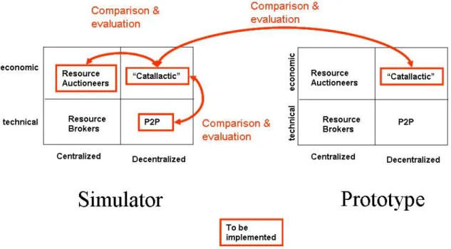
Figure 1.1: Research process for evaluation

Therefore, it is necessary to identify a good procedure that leads to a fundierte eval-uation. This strengthens the explanatory power of the measured and computed results. Figure 1.1 shows the research process. The arrows show the planned comparisons and evaluations, that will be done by the CATNETS project. Further evaluations are not in the scope of the project. Obtaining results from the simulator, we will compare

• first the catallactic approach with common technical approaches in P2P networks and second with centralized resource auctioneers.

• The metrics of the catallactic approach on the OptorSim simulator environment are finally compared with the catallactic approach’s metrics of the prototype environ-ment, supporting the simulated results.

The evaluation of the decentralized catallactic approach with centralized resource auc-tioneers will compare two economic approaches. Preliminary results are evaluated in the predecessor project CatNet [Eym03]. In CatNet, simple centralized resource brokers show scalability problems in large ALNs. This comparison is extended with a more so-phisticated resource broker developed in work package 1 of the CATNETS project. The comparison of the catallactic method with P2P concepts gives feedback of decentralized technical resource allocation strategies which are currently state-of-the-art in P2P net-works. The last evaluation is done between the simulator environment and the prototype. This will give information about whether the results in simulation are close to the results obtained from a real application environment or not. Therefore, the analysis has deep

impact on the adoption of the Catallactic concept in future resource allocation methods in large ALNs.

In the remainder we discuss the evaluation methods and elaborate a framework for measuring resource allocation concepts on ALNs. Proposing economic evaluation con-cepts in a non-trivial way constitutes the important use of economics in the project.

1.2

The method

Basically, the problem of evaluation is how to obtain a single real number indicating the ability of the Catallaxy, that we analyze out of a large amount of information we have that is data from each transaction of each agent. The first idea that comes into our mind is the application of statistics. Statistics are the basic ingredients of our recipe. In simulation studies, the treatment of the output data is important. This analysis phase can involve simple econometrical tools up to refined technics such as the Monte-Carlo analysis [MLW01, Clo, HH79, Rub81].

A relevant problem is that we usually have to evaluate a phenomenon taking into account a set of its features; most important they are not directly comparable because features corresponds to variables of different dimensions and per unity of measurement. One prerequisite is thus to make them comparable.

Once we make them comparable we have to group them into one indicator. An indi-cator is defined as a number or ratio (a value on a scale of measurement) derived from a series of observed facts, which can reveal relative changes as a function of time. This con-sists of choosing a function. But there are infinitely such functions. Thus, this requires an in-depth evaluation step, that is outlined in section 2. In the following, we give a general outline of the methodology used and some examples.

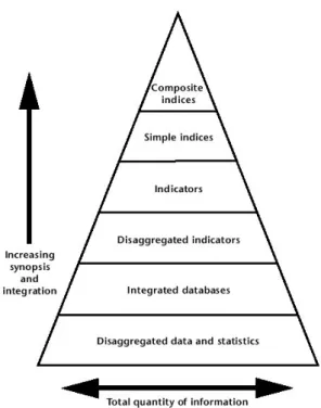
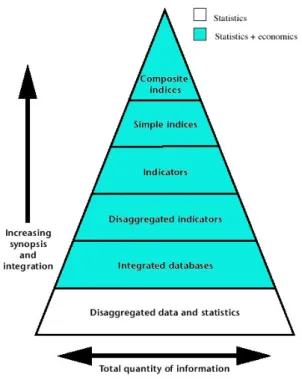
Figure 1.2 shows the logical structure of data and indices and sum up the underlying methodology. In order to evaluate the economic performance of a system, is it needed the largest amount of information The first thing to remark is that going to the upper layer it’s inevitable a loss of information. As first step it’s needed a selection of vari-ables of interests for the evaluation Then, are collected the raw disaggregated data. Since raw data could be collected from different experiment carried out in different condition (space-time) database have to be filtered in order to guarantee the compatibility of data (integrated database). Disaggreted indicators are the first evaluation stage, and are first assembly of variables. Disaggregated indicators are then evaluated together using ag-gregated indicators. latter step is very important because it’s needed some processing of disaggergated indicators which eliminate the heterogeneity in unity of measure. The simplest way is to normalize in some interval and express the indicators as percentage. Finally could be calculated the simple and composite indices.

Simple and Composite indices express information in ways that are directly relevant to the decision-making process. Indicators help assessment and evaluation, but perhaps

CHAPTER 1. INTRODUCTION 6

Figure 1.2: The general method to obtain a composite index from a bunch of data at individual level. Source [ La00] pg. 42.

most important, they help improve accountability. Just as economic indicators, profits or losses can help improve economic accountability, environmental indicators can strengthen environmental accountability.

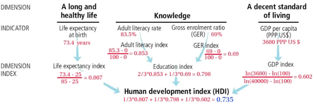
There are a lot of examples of applications of this technics in the social sciences and in economics [Rob93, CHR95]. Here we report a well known application in economics: the Human Development Index (HDI) [UND99]. The problem was to compare standard of living in different countries. For example one of the variable taken into account is of course Gross Domestic Product (GDP), but it is a variable measured with different curren-cies. So comparability is achieved by the conversion of data following the power purchase parity. Figure 1.3 reports the main steps to obtain the HDI. In the figure we can easily recognize our pyramid (it’s just presented in a upside down way). We can also recognize the above illustrated phases of building a Composite Index. Here the disaggregated data selected corresponding to the Dimension layer are Quality of Life, Knowledge and a de-cent standard of living. Disaggergated indicators here correspond to Life to expectancy at birth (73.4 for Albania) or Adult Literacy rate (83.5 As before, this disaggretaed indi-cators bring different information because they belong to different dimension and so are expressed in different unity of measurement (year and percentage). Indicators are then aggregated into simple indices in order to normalize the data (For example the Dimen-sion Index layer for the life expectancy rate equal to 0.807). Finally All the dimenDimen-sion index are aggregated in the Human developemnent index (Composite Index) considering all the dimension of data and indicators. Our main observation here is that a very simple

Figure 1.3: Process to obtain the composite index called Human development Index (data from Albania 2001).

function is used to obtain the final composite index: it’s just an average between different normalized indices.

So while the HDI is a very nice application of the measurement concepts to eco-nomics, there is no application of economic concepts in the measurement process. In the following section we give an idea an how to use economic concepts in the measurement process [Wol88].

1.3

Contemplation of layers

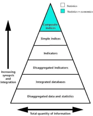
We presented at the end of the previous section a trivial way often used to go from the simple indices to the final composite index (the last level of the pyramid).

A first possibility to insert economic tools in the evaluation process is to use economic concepts instead of a technical one in this final step.

So the evaluation process is divided in two layers (see Figure 1.4). The first one uses only technical or statistical concepts while the second one uses economic principles.

Figure 1.5 summarize the goal of this deliverable. As we pointed out before, the passage from simple indices to the composite index involve a function mapping Rn_into

R. Usually this step is done by means of simple averages so that only a very small subset of the possible functions is used. Our aim here is to search a metrics in a more wide set. The boundary of this new set is “drawn” taking into account economic concepts. So among all the functions mapping Rn into R we want to restrict to these that have an economic sense (this is wider than the averages set). In the following subsection we presents the economic concepts used to identify the “economic” set.

CHAPTER 1. INTRODUCTION 8

Figure 1.4: The two layers pyramid.

1.3.1

Economic concepts

A large part of economics is devoted to understand how agents take decision. But to do that, they must be able to evaluate all the possibilities ranking them in a rational way.

Using these concepts into our problem means that sets of aggregate1_{simple indicesI}

i

has to be compared and ranked. A formal representation is required that indicates that a set of indices is preferred or indifferent to a second one. Having two sets of indices in two situationsaandbwe must be able to establish if

{I₁a, I₂a, . . . , I_na} {I₁b, I₂b, . . . , I_nb},

{I₁b, I₂b, . . . , I_nb} {I₁a, I₂a, . . . , I_na}

or

{I₁b, I₂b, . . . , I_nb} ∼ {I₁a, I₂a, . . . , I_na}

whereand∼means, that the left side set is preferred or respectively indifferent to the right one.

Fortunately, the economists showed that it is possible to describe preferences using mathematical tools (see any book in microeconomic theory for example Mas-Colell et. al [MCWG95] proposition 1.B.2 pag. 9). In particular we can use utility functions. They are analytical functions

Ix =f(I₁x, I₂x, . . . , I_nx)

such that

Ia> Ib ⇔ {I₁a, I₂a, . . . , I_na} {I₁b, I₂b, . . . , I_nb}, Ia=Ib ⇔ {I₁a, I₂a, . . . , I_na} ∼ {I₁b, I₂b, . . . , I_nb},

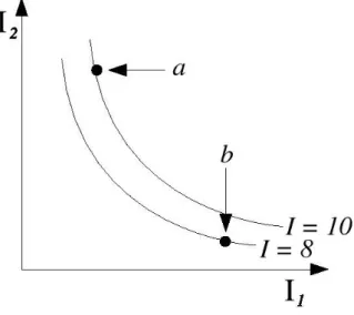
Using a utility function one can identify all the combinations of variables that give rise to a given level of utility. These set are called indifference curves2_{and are commonly}

used in economics. In figure 1.6 two of these sets are depicted in the case only two indices (or goods) are considered.3 The first one (denoted withI = 8 in the figure) relates to a utility level equal to 8 and the second one (I = 10) to a level of utility equal to 10. This representation is useful because combinations that lie in higher indifference curves have higher rank. In this way is very simple to establish that for our agenta b.

In microeconomic theory households and firms are supposed to evaluate alternatives using these tools. Of course we can use them in CATNETS, but a problem arise. Using this concepts we can restrict our choice of the aggregating function from all theRn_→R

function to the one having economic meaning (refer to figure 1.5). But how to choose

1_{See next section for the problem of aggregation.}

2_{This terminology apply to consumption theory. A parallel concept is present in production theory}

where th combination of inputs that ensure a given level of production is called isoquant.

CHAPTER 1. INTRODUCTION 10

Figure 1.6: Choice using a utility function.

among the various alternatives? There is a lot of discretionality in choosing a utility function! We want to avoid this.

There is another possible way to proceed that is more convenient for our purposes and avoid discretionality in choosing an aggregating function. This possibility relates to the policy maker behavior.

We first give the definition of policy maker and policy maker behavior to facilitate the comprehension of people not familiar with economic terminology.

A policy maker is an institution, which manages policies to have better economic performance. Policy maker examples are

• the European central bank and • the ministry of finance

The behavior of a policy maker is a set of rules, a policy maker uses to achieve his goals. To identify these rules three steps are needed:

1. identify a way for measuring system performance (this results in fixing the targets)

2. formulating an objective function or a loss function

3. identify the rules that allow to minimize the loss function

Generally he can intervene with fiscal policy (government) or monetary policy (Cen-tral Bank). In the economic literature a Policy maker behavior is described with an objec-tive function which is to be maximized under some constraint. Constraint is determined

by the structure of the economy or better, the underlying laws of motion of the economy. Moreover, Policy maker has not a complete knowledge of the economy, so he has in mind a model of functioning of the economy which generally is represented by a statistical law. The typical economic example is a policy maker that decide the target levels of the unem-ployment and inflation rates maximizing its objecting function knowing that the Phillip’s curve exists4_{. To achieve the goal the policy maker has instruments (i.e. interest rate or}

money offer) which could be set in order to achieve the target levels.

The problem of a policy maker is similar to this Work Package aim in the CATNETS project, because we have to evaluate different SOAs and in if the organization of ex-changes in a centralized way is better than in a decentralized way.

Changing the perspective from a single agent to the policy maker allows to avoid the discretionality in choosing an aggregating function. Policy makers for each of the n

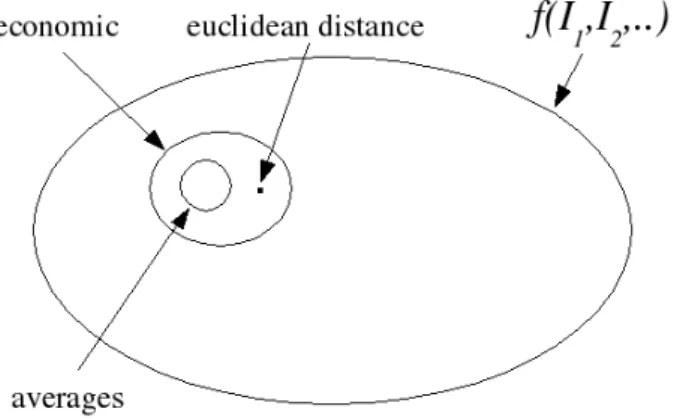
indicators have an perception of what they should be which is defined by their objectives. This is interesting because the goodness of a given situation can be evaluated according to a function giving a distance of the situation from the optimal one. This function is usually called the “loss function”. Of course in this case the policy maker prefers alternatives that reduces the value of the loss function.

So we can write

I =f(I₁−I₁∗, I₂−I₂∗, . . . , I_n−I_n∗)

It is important to note that the f function should be a measure of distance. Taking as reference the Euclidean distance5_{we can now propose to use the following functional}

form:

I =α₁(I₁−I₁∗)2+α₂(I₂−I₂∗)2+. . .+αn(In−In∗)2

where the αs are weights. In this way we avoid the arbitrary to choose a functional form and reduce the arbitrary to the choice of weights. Figure 1.7 illustrate the point.

Graphically the level sets of the loss function are depicted in the figure 1.8.

Obviously combinations ofI₁andI₂closer to the target levelsI₁∗ andI₂∗ have a lower loss. So, in this case we will have

Ia< Ib ⇔ {I₁a, I₂a, . . . , I_na} {I₁b, I₂b, . . . , I_nb},

We will use this approach in the following sections.

4_{The Phillip’s curve is an empirical finding stating that to a high level of inflation corresponds a low level}

of unemployment. It is the constrain of the maximization problem. See every macroeconomic textbook for an introduction to the Phillip’s curve.

5_{Indeed the Euclidean distance is slightly different from the following formulation. The proposed}

func-tional form is an increasing monotonic function of the Euclidean distance, this means that the ranking of the alternatives doesn’t change under this transformation.

CHAPTER 1. INTRODUCTION 12

Figure 1.7: graphical representation of the goal of this deliverable: choosing an aggregat-ing function reducaggregat-ing discretionality.

Figure 1.8: Level sets of a loss function.

1.4

Aggregation of individual level

In our evaluation framework, we won’t analyze the performance at individual level, be-cause our goal is to provide feedback of the system’s behavior as a whole. But, we have to measure the data on individual level. Therefore, we need to aggregate the individual data. The pyramid below shows this process. On the bottom layer we have disaggregated data and statistics for each individual agent, which stores information about his performance. At this layer the quantity of information is highest. Coming to a common data set we need to integrate this data, aggregating the individual data sets. This leads to increased synopsis and adds an economical dimension to the basic data.

Section 2 presents the technical and economical metrics in detail and shows the ag-gregation process from individual data sets to the superior economic value social utility. The sections ends with a description of how this metrics are computed in the CATNETS

Chapter 2

Metric specification and classification

Our goal is to measure and compare the performance in the three scenarios. To achieve this, we have to build an aggregate index available and comparable for these scenarios as discussed in the introduction. Our strategy applies several layers metrics which are configured on a three stage metrics process. As first step, we collect a set of raw data (technical metrics) in order to measure the behavior of agents. At the second stage, we will aggregate the technical metrics in indicators composed in two sets: The on demand availability and infrastructure cost sets. This structure will be useful to analyze further behavioral dynamics about the profitability of the agents. Notice that at this stage, the indicators aggregate information and cross section data about agent behavior. Therefore, we aggregate the indicators in indices, on demand availability and infrastructure costs. Finally, as explained in detail below we will calculate the social utility index.

2.1

Explanation of layers

As already mentioned, we structure the metrics in two main layers: a technical layer, and an economical layer. The total quantity of information reduces at each layer through aggregation and composition. This leads to a pyramid-like graphical form, whereas the width indicates the quantity of information. At the same time the view of the system gets a broader granularity.

We identify two two main objectives of the performance measuring framework for service oriented architectures:

• On top, the social utility value characterizes the the ALN of a specific organization (bank, retail company, small office, etc.), hiding lower level details. The quantity of information can be aggregated to only one value, which shows the welfare of the system.

• The technical parameters enable a non-economical evaluation of the proposed sce-14

narios.

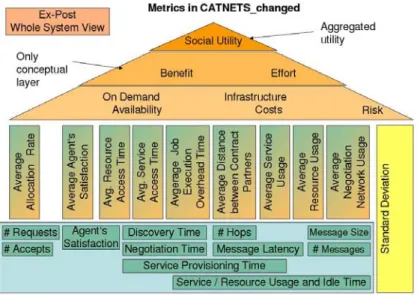
Figure 2.1 shows the metrics pyramid we propose for analyzing the performance of a SOA. The pyramid is layered from top to bottom, representing economic parameters above and technical below. Lower level parameters contribute qualitatively and quantita-tively to the above values.

Figure 2.1: The metrics pyramid

The top layer of the pyramid presents the superior economic value utility which should be taken into account as index for comparing several alternatives. Utility can be calcu-lated by benefit and effort. Benefit can be expressed by on-demand availability. Effort by the required infrastructure costs and the risk that has to be taken. The average allocation rate embodies the ratio of the number of requests and accepts and in combination with the agent’s satisfaction related to whether the agents can fulfil their requirements in terms of QoS-guarantees. Service/Resource access time represents the waiting period, calculated as the time frame between the identification of a service/resource need and the actual ser-vice usage, including discovery time and negotiation time. Job execution overhead time is the sum of access times when accessing a set of services/resources. These time values, the allocation rate and the satisfaction contribute to the on-demand availability metric. The distance between transaction partners is measured together with negotiation network usage for identifying the infrastructure costs. Service/Resource idle times represent the efficiency of the provision to the market.

The first technical layer is a measure of the event of interest (please describe further) and the behavior of agents together with information about the performances of markets. These data are collected for each individual agent and are selected with the criteria to measure the benefits and costs which each agent can incur in the selected scenario. In

CHAPTER 2. METRIC SPECIFICATION AND CLASSIFICATION 16 order to evaluate the distribution of this data across population of agents, we will evaluate the cross section standard deviation of this variables.

The economical layer is composed of two sub-layer: the aggregation layer, where we evaluate the means and some composite indicators, and the benefit and cost layer where we aggregate the aggregation layer’s metrics data.

2.1.1

Technical layer

Technical layer is selected in order to evaluate the benefits and costs of participation for each individual layer. They can be classified in efficiency measures (number of request, number of acceptance) and utility measures (agent satisfaction). Together, they are a measure of technical benefit which agents earn. Another set is the time metrics (discovery time, negotiation time, service provisioning time) which are measures of the velocity of market processes. Messages metrics are included in order to measure the activity of agents to communicate to find resources and services.

Here we enumerate the single technical metrics:

1. Number of Requests: This metrics counts the number of demanded services, which are Basic Services and Resources in the CATNETS scenario. Therefore, we mea-sure the number of requested Basic Services and Resources.

2. Number of Acceptance: The number of acceptance meters the successfully re-quested services. As described above this is done on the Service and on the Re-source market.

3. Agent Satisfaction: The individual agent satisfaction measures the gain followed by any single transaction. It’s a measure about Complex Service and Basic Service and is defined as the ratio between the subjective quality requirements and price. Each item regarding a transaction is defined by a couple price-quality. The agent’s satisfaction represents in CATNETS the individual utility of an agent. Here, we show an example transaction at the negotiation stage; A complex service addresses 3 basic services which state a price for the service and their quality. Satisfaction is the ratio between quality and price; Ex post satisfaction is calculated as the actual and final satisfaction occurring with the acquired service (it is normalized with the best available service addressed from complex service).

Price QoS Satisfaction rank BS1 10 12ms 70% 2 BS2 7 15ms 50% 3 BS3 12 7ms 100% 1

4. Discovery time: In generally, this metric defines the time to find a given set of possible negotiation partners. In CATNETS this time is twofold: First, it is the time a Complex Service needs to find available sellers and second it is the time a Basic Service needs to find resources. These two times are summed up to measure the whole discovery time.

5. Negotiation Time: The negotiation time meters the time needed to finish the nego-tiation between one buyer (service consumer) and sellers (service provider). The measurement of the negotiation time starts after the service discovery and ends be-fore service usage or service provisioning.

6. Service Provisioning Time (Effective Job Execution Time): The evaluation frame-work defines the service provisioning time as the service usage time of one transac-tion. It optionally includes also setup times, etc.. In CATNETS, this time is fixed to a given value, because this time would falsify the negotiation and discovery times and is not in the focus of the project evaluation.

7. Application Data Network Transfer Time: This time corresponds to the amount of data transferred over a network link after the negotiation phase ended and a contract was closed. It is the data the service/resource uses for computation. The amount can range from a few bytes in the case of a computational or search service up to gigabytes in data intensive services like multimedia applications or data grids.

8. Total Job Execution time: This time includes all times for one complex service usage. In detail, the total job execution time is defined as a sum of these time pa-rameters: discovery time, negotiation time, network transfer time and provisioning time. Compared to the job execution overhead time, this time parameter also in-cludes the execution related time metrics network transfer time and provisioning time.

9. Hops: The number of hops describes the distance from a service consumer and a service provider counting the number of nodes the messages have to pass. This value is defines an absolute quantity.

10. Message Latency: The message latency measures the time in [ms] a message needs to arrive the communication partner. Message latency is a parameter that indicates the performance of the physical network link and its message routing capabilities. It is expected that high distance (see number of hops above) between a service consumer and service provider will lead to a high message latency.

11. Message Size: This parameter sets the message size in [kb]. We will measure realistic values in the CATNETS prototype and use this value in the simulator.

12. Number of Messages This value counts the number of messages needed for service allocation. The traffic on a physical network link is simply computed by multiplying the message size with the number of messages sent.

CHAPTER 2. METRIC SPECIFICATION AND CLASSIFICATION 18

2.1.2

First Aggregation of technical layers

In this section we discuss the first level of aggregation. As illustrated above, this layer is structured into two sub layers: the simple indicators layer and the composite indicator layer.

CATNETS simple indicators layer This layer is a set of indicators which are a measure normalized between zero and one. This is done because, we want to isolate the effect of the metrics’s unities which are not homogeneous.

The only assumption we do is common is statistics that is all the the basic variables are independent. The assumption makes it easier to find functions for the layers above: on demand availability, infrastructure costs, risk. We know at the current state of the project no well defined dependencies. Thus, we plan to use data mining tools in the later stage of the project for analyzing dependencies and refining the formulas.

The discussion here is developed at the theoretical level. Indeed here we point out that all the basic technical variable can be viewed as statistical distribution. At a theoret-ical level we can refer to them as random variables. We highlight this fact denoting the variables with capital letters.

Basically here we show how the technical metrics are successively mixed to obtain a framework that allows a final evaluation different SOAs.

The aggregated metrics at the CATNETS simple indicator layer are:

1. Allocation Rate: this aggregate the individual allocation rates on the service and resource market. It is a measure for the efficiency of the allocation process, which is computed using the number of requests and number of accepts. A buyer can demand services, but it’s not granted that the allocation mechanisms (centralized or decentralized exchange) performs a matching between demand and offer. We denote it with

ALLOC.RAT E

2. Agent’s Satisfaction: The individual agent’s satisfaction is aggregated into the sim-ple indicator agent’s satisfaction. This metric implicitly shows the fitness of the agents in the system. A low value means that the agents have problem in reach-ing their individual goals durreach-ing the negotiation process. A high value means that the agents in the system can constitute good results satisfying the demands. in the following we refer to this variable as

AGEN T.SAT ISF

3. Access Time: This indicator evaluates the time needed for the agent population from the starting point of discovery until the final delivering of the service and available for the Complex Service or Basic Service.

ACCESS.T IM E =DISCOV ERY.T IM E +N EGOT IAT ION.T IM E+

+P ROV ISION IN G.T IM E

4. Job Execution Overhead Time: This is the total time additionally needed for nego-tiation. It refers to the overhead introduced using service negonego-tiation. The overhead is the sum of the service market access time and the resource market access time.

J OB.EXECU T ION.OV ERH.T IM E =ACCESS.T IM ESERV ICE.M ARKET+

+ACCESS.T IM ERESOU RCE.M ARKET

From the point of view regarding infrastructure costs we will measure the message latency and the network usage, i.e. the effectiveness of usage form agent’s of the network

5. Distance between Contract Partners: Message latency would be the messaging time incurred to agents and it is proportional to distance between sending and receiving nodes. The latter would be the ratio between the actual distance and the maximum distance between agents.

DIST AN CE =LIN KS.BET W EEN.CON T RACT.P ART N ER

6. Service/Resource Usage: The network usage will be evaluated by the ratio between the provisioning individual time and the total simulation time occurred until the evaluation This evaluation would be done for both resource and service market.

SERV ICE.U SAGE =

_{P ROV ISION IN G.T IM E}

simulation.time

RESOU RCE.U SAGE =

_{P ROV ISION IN G.T IM E}

simulation.time

remember that capital letter denote distributions while lower case denote real num-bers.

7. Network Usage: Finally, in order to evaluate the message exchange activity, We evaluate the quotas of messages across population.

N ET W ORK.U SAGE = #M ESSAGESS∗messages.size

CHAPTER 2. METRIC SPECIFICATION AND CLASSIFICATION 20

2.1.3

Second aggregation

Once evaluated the simple indicators, we aggregate them into composite indicators. Sim-ple indicators are normalized between (0,1) interval in order to be compatible within them. From the economical point of view, those indicators measure the benefits from ex-change (or the on demand availability), and costs incurred from activities into the market (infrastructure costs). Summarizing we will have the following composite indicators

ODM = on demand availability IC = Infrastructure cost

On demand availability (ODM) is a composite indicator obtained as mean of 1., 2., 3., and 4. simple indicators, i.e.

ODM = 1

4(ALLOC.RAT E+AGEN T.SAT ISF+

+ACCESS.T IM ESERV ICE+ACCESS.T IM ERESOU RCE) (2.1)

Infrastructure costs (IC) is calculated in the same way. It is the mean from 5., 6., 7., 8. and 9. simple indicators:

IC = 1

4(DIST AN CE+SERV ICE.U SAGE+RESOU RCE.U SAGE+

+N EGOT IAT ION.N ET W ORK.U SAGE) (2.2)

Let us highlight again that the variables we have now can be interpreted as random variable. Of course knowing the shape of the random variable is very useful but take with it a lot of trouble. Usually the bunch of information born by random variables are collapsed into one or two statistics. The first step is to consider the mean and the variance (or standard deviation).

Indeed the variance is very important because signals how far from the average value one can expect to have realizations of the random variable. In several economic applica-tions the variance is given the meaning of risk.

In the following section we outline the way we use to go from distributions to a real number that give the performance of the system. This is done in two steps:

1. use a Euclidean like distance function to summarize the two distributions

2. show how this can result in a function of the means and variances

As we will see this process is used in macroeconomic theory, so that the use of eco-nomic layer is sound justified at this level.

2.1.4

The final formula

In order to enable the comparability of the scenarios, in this section we show the theoreti-cal framework and the structure of the aggregate index. It should be an aggregate measure of ODM1_{and IC.}

As mentioned in the introduction there are an infinity of ways (functions) to get from the simple index to the composite one. In a large number of applications atechnicalway is followed using simple averages (for instance in the HDI).2

CATNETS ECONOMIC composite index In order to bring economic concepts into the evaluation process, we use the policy metrics loss function we talked about in the previous section. Our policy maker (social planner) collects all the previous metrics. It has some preferences about ODM and IC and is aware about the distribution of the benefits and costs. Here, we can take as reference an approach which was developed in Macroeconomics.

But before entering into details let us give some hint about two existing macroeco-nomic models (Barro and Gordon 1983, Poole 1970).

Monetary Theory Barro and Gordon [Bar83] is an economic model describing a social planner which decides on his policy.

The central bank is aware of the equilibrium level, the inflationπ, and productiony∗. The social planner obtains these data and uses a loss functions L to decide upon policy rules

L=θπ2+ (y−y∗)2

whereθ is a weight, π is the rate of inflation, y = f(Y)is a function of the Gross Domestic Product and y∗ the policy maker optimal value of y. The loss function is a distance function from the point(0, y∗).

Risk in monetary Policy Barro Gordon build a deterministic model assuming that the policy maker knows exactly the functioning of the economy. Performing a relaxation of this hypotheses, Poole [Poo70] allows for a more precise knowledge in term of statistical

1_{Indeed below we demonstrate the need to insert ODM as the difference by one (1-ODM).}

2_{For CATNETS a technical composite index could be a weighted mean between them with weightsα,}

β,γwhereα+β+γ= 1.

I=αODM+βf(IC) +γf(Δ)

CHAPTER 2. METRIC SPECIFICATION AND CLASSIFICATION 22 distribution of the relations between objective variables. If y is a stochastic variable the loss function without inflation becomes

L=E[(y−y∗)2]

.

Following the particular hypothesis adopted by Poole, we obtain

y−y∗ =u

whereuis a random variable with mean equal to zero (μ_y = 0) and positive variance (σ_y2 >0).Then, Substituting in the loss function we have

L=E[u2]

but according to a basic statistical rule

E[u2] =σ2_y

The policy maker problem is

minσ_y2

Therefore, the objective is to minimize the variability of the model.

Discussion of the models With the policy maker, presented in introduction we refer to an economic agent who has the role to improve the economic welfare of a society. Generally he can intervene with fiscal policy (government) or monetary policy (central bank).

In our case the Barro Gordon model refers to a central bank which has to maximize its objective function considering inflation and production. Production and inflation are linked by a trade-off relation; for example the central bank could have the impression that the economy with a lower inflation has a lower production and vice-versa. If the central bank (policy maker) wants to improve production it has to accept a greater inflation. To achieve the goal the central bank has an instrument (i.e. interest rate or money offer) which could be set in order minimize inflation or maximize production. Then, he has to decide the optimal level of his instrument.

In the Poole model, the central bank has an objective function which could be inter-preted as the distance between the optimal value of production and the actual one. Since

the knowledge of the economy is summarized by the statistical law which state that the difference of actual production by the optimal value is a random number, then substitut-ing it into the objective function the goal of Central bank became the minimization of variability of production. This means that the welfare of society is improved, lowering the fluctuation of the economy. In the mapping, we assume that the optimal value of X and Y are zero, so the CATNETS social planner has to achieve those values. It means that if the social planner minimizes the inverse ODM and IC i.e. reducing the distance to zero of those variables, the welfare is improved. Moreover, he knows that X and Y are distributed across population (i.e. he knows the statistical moments [mean and the variance] of those variables) in the sense that he looks at the distribution of benefits and costs over the agents. Then a result of the final optimization rule is that the social planner is interested to minimize inequality between agents. So risk in our case is interpreted as an equality measure of welfare.

Application to CATNETS In order to follow this approach into the CATNETS project, we could build a loss function where the arguments are ODM and IC. This time ODM and IC are taken as stochastic variables and so are considered their distribution across population by the first and second moments (mean and standard deviation). Renaming the variables for the presentation

X = inverse on demand availability index Y= costs index

the CATNETS loss function is

L=E[α(X−X∗)2+β(Y −Y∗)2]

whereα andβ are weights andX∗ andY∗ are target values. It is important to give a values to the targets. Remembering thatX is the inverse of the On Demand Availability we can conclude that the lower it is the better is for the policy maker. So we take the target values equal to zero (X∗ = 0). Y is a direct measure of costs so it is natural to choose zero even for this variable (Y∗ = 0). With this targets the loss function is

L=E[αX2+βY2]

our random variables can be expressed as

1.

X =μX +u

2.

CHAPTER 2. METRIC SPECIFICATION AND CLASSIFICATION 24 where u and z are random variable with zero means and positive variances (μu =

0, μz = 0, σ2u > 0, σz2 > 0). Note that variances σu2 and σz2 are the variance cross

population. Substituting 1. and 2. into the loss function and proceeding with the following passages we obtain the final social utility index

L=E[α(μX +u)2+β(μY +z)2] L=E[αμ2_X +α2μXu+αu2+βμ2Y +β2μYz+βz2] L=αμ2_X +α2μXE[u] +αE[u2] +βμ2Y +β2μYE[z] +βE[z2] L=αμ2_X +α2μXμu+ασu2 +βμ2Y +β2μYμz+βσ2z remembering that (μu = 0, μz = 0) L=αμ2_X +ασ_u2+βμ2_Y +βσ2_z

So one possibility for CATNETS is

minαμ2_X +ασ2_u+βμ2_Y +βσ_z2 (2.3) This means that for the final evaluation of the scenarios we have to evaluate the first and second moments of ODM and IC, whereas the first moment is the mean of ODM and IC and second moment the variance of ODM and IC. In fact a social planner, has preference and objective to minimization of the inverse of ODM, the minimization of costs and the minimization of variability, i.e. the fair distribution of welfare between agents.

The following section shows how it is possible to calculate the averages and variances we need to compute the metric.

2.2

Obtaining results

2.2.1

General method

In this section we will discuss about the general method used to collect each single met-rics, from the technical level to the aggregated index. The data are collected for each

individual i. This means that for each individual agent a set of variables for the techni-cal layer will be collected; we remind that the only data originated from the simulator and prototype are that lying in the technical layer and thereafter, they will be aggregate following what shown above.

As we are interested to evaluate the aggregated index L which is a function of the means and variances of costs and benefits, it could be that the progressive aggregation of data made over the metrics layers, cause a loss of information ,or worst, a misrepresen-tation of the functioning of the system. In order to avoid this situation, fortunately, we can utilize sample theory. This fundamental result state that, considering a set of random variables with arbitrary distributions with finite variance, identically and independently distributed, and the sum of them, the latter will have mean and variance as linear combi-nation of the moments of the variables summed. This grant that the indexLis correct and representative. Each technical layer is collected for each transaction. From this assump-tion for each technical are obtained 2 dimensional data, one for individuals and one for transactions.

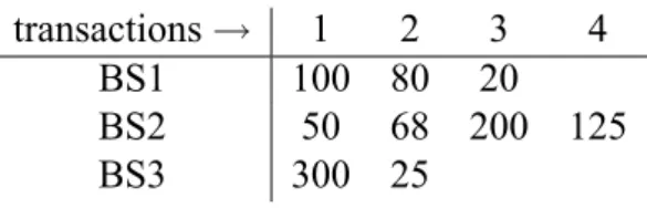
(a) Data

The goal is to obtain a collection of data (technical layer) which could be interpreted as experiments. We interpret each individual agent as an indepen-dent experiment from which are take the observations of the set of metrics. Each individual will be oberserved for each transaction occurred. The results are two dimension technical metric series. In table 2.1 is depicted an exam-ple for an hipotetical technical metrics. For each agent (Basic Service) and transactions, are collected the data obtaining the following tables

transactions→ 1 2 3 4 BS1 100 80 20 BS2 50 68 200 125 BS3 300 25

Table 2.1: data

we use the notationaitto indicate the entry in the table corresponding to row

iand columnt. (b) Normalization

The normalization can be done using each function that maps into the interval [0,1]. In this example let us use the very simple following expression

an_it= ait a_max

where the superscript n means “normalized”. the normalized data are pre-sented in the following table

CHAPTER 2. METRIC SPECIFICATION AND CLASSIFICATION 26 transactions→ 1 2 3 4 BS1 0.333 0.266 0.066 BS2 0.166 0.226 0.666 0.416 BS3 1 0.083 (c) Summary variables

Remembering the discussion in the previous section what we need out of these data are two values: the mean (μA) and the variance (σA2). As pointed out

before to obtain these values we can use samples theory. Each row of a matrix can be interpreted as a sample of the relative random variable. We denote a row asai. So we identifya₁, a₂ anda₃ as the first, second and third sample

of the population.

For each sample we can compute average and variance.

transactions→ 1 2 3 4 μ σ2

BS1 0.333 0.266 0.066 0.222 0.0129 BS2 0.166 0.226 0.666 0.416 0.368 0.317 BS3 1 0.083 0.541 0.21

Samples theory tell us that3

μA=E μan_i = 1 m m i=1 ⎛ ⎝1 Ti T_i t=1 ait a_max ⎞ ⎠ (2.4) and σ2_A=Eσ_a2 i = 1 m m i=1 ⎛ ⎝1 Ti T_i t=1 _a it a_max −μani ₂⎞ ⎠ (2.5) where Ti is the number of transactions of agent i and m is the number of

agents. Numerically we obtain μA= 0.376 and σ_A2 = 0.18 (d) Further Aggregation

In some case the indicators are composed by more than a variable. Indeed they are sums or weighted sums. Suppose we have the following variable

X =

j

αjAj

3_{The result for the mean is exact, the one for the standard deviation is a good approximation if one}

basic statistics tell us that μX = j αjμA_j and σ_X2 = j α2_jσ2_A j

provided that theAj are independent.

2.2.2

Application

For each of the 7 variables identified in section 2.1.2 we describe how to apply the general method if it is possible and provide the way to collect data and perform calculation in the cases it is not possible to apply.

1. Allocation rate

(a) Data

In this case presenting the data as in table 2.1 has little sense (so this is a case where we cannot apply the general method). So we start from a different data format: requests accepts CS1 200 100 CS2 100 100 .. . ... ... (b) Normalization allocation.raten_i = #acceptsi #requestsi alloc.raten i CS1 0.5 CS2 1 .. . ... (c) summary variables μa.r = 1 m m i=1 #acceptsi #requestsi σ_a.r2 = 1 m m i=1 #acceptsi #requestsi −μa.r ₂

CHAPTER 2. METRIC SPECIFICATION AND CLASSIFICATION 28 (d) Further aggregation

none

2. Agents’ satisfaction

(a) Data

Matrix. the format is equal to the one in table 2.1. (b) Normalization

The data are already normalized between 0 and 1.

agent.satisf actionn_it =agent.satisf actionit

(c) summary variables μage.sat=E μan_i = 1 m m i₌₁ ⎛ ⎝1 Ti T_i t₌₁ agent.satisf actionit ⎞ ⎠ and σ_{agents.satisf action}2 =Eσ2_a i = 1 m m i=1 ⎛ ⎝1 Ti T_i t₌₁

(agent.satisf actionit−μage.sat)2

⎞ ⎠

(d) Further aggregation

none

3. Access Time

(a) Datawe need the following data:

variable format unit of measure

discovery.time table 2.1 milliseconds

negotiation.time table 2.1 milliseconds

provisioning.time table 2.1 milliseconds (b) Normalization

Time can be very large and have no upper bound. To normalize we need a function mapping[0,∞]→[0,1] Possibilities are x.timen_it = 1 1 +x.timeit or x.timen_it =e−βx.timeit

where xcan be substituted with discovery, negotiationand provisioning, andβ is a parameter.

(c) Summary variables

For the discovery time

μd.t =E μan_i = 1 m m i₌₁ ⎛ ⎝1 Ti T_i t=1 discovery.timen_it ⎞ ⎠ and σ_d.t2 =Eσ_a2_i= 1 m m i=1 ⎛ ⎝1 Ti T_i t=1 (discovery.timen_it−μd.t)2 ⎞ ⎠

For the negotiation time

μn.t =E μan_i = 1 m m i=1 ⎛ ⎝1 Ti T_i t=1 negotiation.timen_it ⎞ ⎠ and σ_n.t2 =Eσ_a2 i = 1 m m i=1 ⎛ ⎝1 Ti T_i t₌₁ (negotiation.timen_it−μn.t)2 ⎞ ⎠

For the provisioning time

μp.t=E μan_i = 1 m m i=1 ⎛ ⎝1 Ti T_i t=1 provisioning.timen_it ⎞ ⎠ and σ_p.t2 =Eσ2_a i = 1 m m i₌₁ ⎛ ⎝1 Ti T_i t₌₁ (provisioning.timen_it−μp.t)2 ⎞ ⎠ (d) Further aggregation

As mentioned in the previous section the access time in the sum of the three times so (assuming they are independent) its mean and variance is

μa.t =μd.t+μn.t+μp.t

σ2_a.t=σ2_d.t+σ2_n.t+σ_p.t2

4. Job execution overhead time

This variable is the sum of the access times of the service and resource markets. The summary variables can be obtained from the previous one doing an aggregation step so we have

μjob.exec.overh.time =μaccess.time.serv.mark +μaccess.time.resou.mark

and provided the two access time are independent

CHAPTER 2. METRIC SPECIFICATION AND CLASSIFICATION 30 5. Distance between contract partners

(a) DataMatrix. the format is equal to the one in table 2.1. (b) Normalization

links.between.contractP artenern_it= links.between.contractP artenernit

#agents (c) Summary variables μlink.bet.contr.part =E μan_i = 1 m m i=1 ⎛ ⎝1 Ti T_i t=1 links.between.contractP artenern_it ⎞ ⎠ and σ_{link.bet.contr.part}2 = 1 m m i₌₁ ⎛ ⎝1 T_i T_i t=1

(links.bet.contr.P artn_it−μlink.bet.contr.part)2

⎞ ⎠

(d) Further aggregation

none

6. Service/Resource usage

(a) DataMatrix. the format is equal to the one in table 2.1. (b) Normalization

x.usagen_it= provision.timeit simulation.time

wherexstands for service or resources. (c) Summary variables μx.usage= 1 m m i=1 ⎛ ⎝ 1 Ti T_i t=1 provision.timeit simulation.time ⎞ ⎠ and σ2_x.usage= 1 m m i=1 ⎛ ⎝ 1 Ti T_i t=1 _{provision.time} it simulation.time −μx.usage 2⎞ ⎠ (d) Further aggregation none 7. Network usage

(a) Data Matrix. the format is equal to the one in table 2.1. Data are integers denoting the number of messages needed to conclude a negotiation.

(b) Normalization

network.usagen_it= #messagesit∗messagess.size

#massages∗messages.size (c) Summary variables μnet.use = 1 m m i=1 ⎛ ⎝1 Ti T_i t₌₁ #messagesit∗messagess.size #massages∗messages.size ⎞ ⎠ and σ2_net.use= 1 m m i=1 ⎛ ⎝1 Ti T_i t₌₁ #messagesit∗messagess.size

#massages∗messages.size −μnet.use

₂⎞ ⎠

(d) Further aggregation

none

2.2.3

The final formula

Now what we have to do is to find averages and variances of the X and Y random variables and substitute them in equation 2.3.

We remember that

X = 1−ODM

and

Y =IC

Substituting the definitions of ODM and IC we gave in equations 2.1 and 2.2 we have

X = 1− 1

4(ALLOC.RAT E+AGEN T.SAT ISF +J OB.EXECU T ION.T IM E)

and

Y = 1

4(DIST AN CE+SERV ICE.U SAGE+RESOU RCE.U SAGE+

+N EGOT IAT ION.N ET W ORK.U SAGE)

Applying statistics theorems we can write

μX = 1−1

CHAPTER 2. METRIC SPECIFICATION AND CLASSIFICATION 32 Next we need the variance ofu=X−μX, but from statistics we know thatσu2 =σ2X

so that

σ_u2 =

₁

4

₂

(σ_a.r2 +σ2_agent.sat+σ_{job.overh.exec.time}2 )

For infrastructure cost we have

μY = 1

4(μdistance+μsevice.use+μresouce.use+μnet.usage)

and

σ_z2 =

₁

4

₂

(σ2_distance+σ_sevice.use2 +σ_resouce.use2 +σ2_net.usage)

finally substituting in equation (2.3) we get

minα

1− 1₄(μa.r+μagent.sat+μjob.overh.exec.time)

₂ + +α ₁ 4 ₂

(σ_a.r2 +σ2_agent.sat+σ_{job.overh.exec.time}2 )

+ +β

₁

4(μdistance+μsevice.use+μresouce.use+μnet.usage)

2 + +β ₁ 4 ₂

(σ2_distance+σ_sevice.use2 +σ_resouce.use2 +σ_net.usage2 )

Conclusion and future work

In this deliverable the design of a general performance measuring framework for resource allocation in ALNs has been largely accomplished. This framework enables performance measurements and evaluations on system level in service-oriented architecture.

The evaluation process becomes a mayor focus in the CATNETS project, since its results will allow to evaluate our approach. The presented performance measuring frame-work suggests a rich set of technical and economic parameters, which should allow eval-uating the middleware at various levels, ranging from determining local node behavior up to global performance. While the parameters in the lower levels of the pyramid provide technical data, higher level economic parameters could be integrated into business models for decision makers.

However, the implementation and possible refinements of the presented concept is ongoing work, which will be done in the later stage of the project. We have defined three scenarios in our evaluation process. An exact specification about how to measure the defined metrics in these scenarios and integrate them is also ongoing work which will performed in the next few moths.

There are two possible improvement of the metric evaluation. The first one is to enrich the previous scheme to take into account more detail about of the distribution involved. Of course the previous analysis is a step ahead of considering only averages values. Here even the dispersion of the phenomena are taken into account by means of the variance. But of course averages and variances are only two aspects of a complex phenomena. To better understand let us give an example. Suppose we have to describe a person. What we did here is to give a description based on height and weight (think of this as average and variance). While this can be considered a sufficient condition it is clear that better ones are possible. A first possibility at a statistical descriptive level is to perform a quantile analysis (median-three quarter analysis).

The second possibility is to introduce economic concepts in a very early level: at the basement of the pyramid. Until now we have just choose the scenario that maximises an aggregate loss function. Here the aggregation is for a large part performed at technical

CHAPTER 3. CONCLUSION AND FUTURE WORK 34 level. A further possibility is to use the scheme in figure 3.1

Figure 3.1: The two layer pyramid with utility at the microeconomic level.

According to this second possibility one can compute utilities for each single agent starting from the technical metrics at the basement of the pyramid. Obtaining these utili-ties (ui) one can proceed with the analysis of their distribution and performing aggregation

starting from them.

This is a very relevant problem in microeconomics studied since more than a century. To give an idea of the method let us give the following example. Suppose we have to choose between the two situations. Suppose their technical data (i.e. prevision time etc.) are the same. To have an idea on what could be the added value of this method note that the two situations are equivalent using the macroeconomic composite index built in this deliverable. We demonstrate here that using utilities at the individual level the evaluation of the two situation can change.

Suppose we give the agents an individual utility function:

ui =f(xi)

wherexiis a technical metric.

Standard assumption on the derivatives of this function are:f >0andf <0. Take for example this function

Suppose further that the two situation we have to compare are:

• situation 1xbuyer = 4andxseler = 4

• situation 2xbuyer = 6.5andxseler = 1.5

Calculating utilities for the first situation we have:

ubuyer = 40.5 = 2

useller = 40.5 = 2

Assume now that the welfare is the sum of the individual utility:

Wf irst example = 4

For the second situation we have

ubuyer = 6.50.5 = 2.55

useller = 1.50.5 = 1.225

so that

Wsecond example = 3.775

So if we first aggregate and the consider utility we have

Wf irst example i xi =Wsecond example i xi

while first considering utilities and the aggregating lead to a different conclusion

Wf irst example > Wsecond example

In the future work we want to find out if this second is possible and appropriate to perform evaluation in the CATNETS project.

Bibliography

[ La00] Laszl´o Pint´er and Kaveh Zahedi and David R. Cressman . Capacity Build-ing for Integrated Environmental Assessment and ReportBuild-ing. International Institute for Sustainable Development and United Nations Environment Pro-gramme, 2000.

[Bar83] Barro, R. and Gordon, D. Rules, Discretion and Reputation in a Model of Monetary Policy. Journal of Monetary Economics, 12:101–122, 1083. [CHR95] C. Cobb, T. Halstead, and J. Rowe. The genuine progress indictor:

Sum-mary of data and methodology. San Francisco: Redefining Progress, 1995. [Clo] ClockworkSolutions. Analytical methods versus the monte carlo method.

www.clockwork-solutions.com/marketingpdfs/AnalyticalMonteCarlo.pdf.

[Eym03] Eymann, T. and Reinicke M. and Freitag, F. and Navarro, L. and Ardaiz, O. CATNET Project: Catallaxy Evaluation Report. Report No. D3. Barcelona. Technical report, UPC Barcelona and University Freiburg, 2003.

[HH79] J. Hammersley