Based on the Correlation of the File Dynamic Replication Strategy
in Multi-Tier Data Grid
Zhongqiang Cui
1,2, Decheng zuo
1and Zhan Zhang
11
School of Computer Science and Technology, Harbin Institute of Technology,
Harbin, China
2
Department of Information Engineering, ShiJiaZhuang University of Economics,
ShiJiaZhuang, China
[email protected], [email protected], [email protected]
Abstract
The data grid is one of the infrastructures for data and storage resource management. Data replication can improve data access performance, fault tolerance, and reduce network transmission bandwidth. As the site storage space is limited in the grid, how to effectively use grid resources become an important challenge. This paper introduces a dynamic grid replication algorithm based on popularity support and confidence (BPSC). Through the algorithm, data and its associated copy can be placed on a suitable site, with reduced access latency. Through Optorsim, simulation results show that the algorithm can provide better performance compared with other algorithms
Keywords:data grid, confidence, popularity, support, Optorsim
1.
Introduce
Grid computing is an important branch of distributed computing. Grid computing constructs a virtual computer system through using a different location of the large number of heterogeneous resources (CPU and storage), provides the model to solve the problem of large scale computing and storage. The data grid is mainly the grid for data storage management. The data grid is defined as an effective combination of data and computing resources of distributed systems by Data Grid Group. The large-scale data-intensive applications, such as bioinformatics, high energy physics, space information generated vast amounts of data, these data may be TB scale, even up to the scale of PB. It is not practical to maintain large scale data at each site, and provide computing resources for visitors. At the same time, it will lead to increased access latency through a centralized way to storing and accessing these data from each site.
Data replication technology is an effective method to reduce access latency in the data grid system. Data replication is one of the basic methods of distributed systems to improve the efficiency of system access, maintenance, system high availability. Data replication is to store data in the appropriate site for users to effective access to massive data. Data replication can reduce data access latency, reduce network bandwidth consumption, avoid congestion, adjust the load balancing in server-side, improve system reliability.
Many data replication algorithm can reduce data access latency, improve system reliability, but which data will be copied, when the data will be copied at, where the data will be copied are the basic means of determining data replication algorithm. In this paper, we introduced a real-time dynamic data replication algorithm. The algorithm is based on the popularity of file dynamic to replicate data, and consider the storage space limitations of the site. Through optorsim simulation verified the algorithm.
This paper is organized as follows: Section 2 is about related works on replication in data grids. In Section 3, system model and component in system are presented. The file
dynamic algorithm are presented in Section 4, and Section 5 is the simulation results , the final in Section 6 is conclusion.
2.
Related Work
Ranganathan and Foster [1, 2] present 6 dynamic data replication strategies in data grid. They are:
1) No Replication: data are only stored in generated node and are not replicated in other nodes;
2) Best Client: each node records the requests for its files and checks this record at regular intervals. If the number of requests for a file exceeds the threshold, the replication mechanism replicates this file in a node which has the higher file requests. This node is called the best client;
3) Cascading: if the number of accesses for a file exceeds the threshold, a replica is created at the next level on the path to the best client;
4) Plain Caching: the client that requests a file stores a copy locally; 5) Caching plus Cascading: combines plain caching and cascading;
6) Fast Spread: the requested file is replicated in all nodes on the path from the source to the destination.
They introduced three kinds of localities:
1)Temporal (time) locality: recently accessed files are much possible to be requested again soon;
2)Geographical (client) locality: recently accessed files by a client are likely to be requested by adjacent clients, too.
3)Spatial (file) locality: related files to recently accessed file are probable to be requested soon.
The simulation results show that the fast spread has a good performance in the random access mode, and it saves more bandwidth than other strategies. Cascading strategy showed better performance when there are more localities.
M. Tang, and B.S. Lee presented two kinds of dynamic replication algorithms in multi-tier data grid: simple bottom up (SBU) and aggregate bottom up(ABU) algorithms[3]. SBU algorithm is that each site of the middle layer copy a replica from up lay according to the popularity of file, however, SBU does not consider historical accesses. The ABU algorithm is that each middle layer site statistics the same file of access number and computing popularity from the underlying lay, ABU considers the access histories of files. They compares the SBU, ABU, fast spread algorithms through simulation, the results show ABU algorithm has a better performance in the average response time than SBU and fast spread algorithm. Unfortunately, significant storage spaces are used.
Lin et al., [4] address the problem of replica placement in hierarchical Data Grids considering locality requirements in Data Grids. They calculate the optimal number of replicas through the maximum workload capacity of each server and then distribute the replicas across servers so that the workload on each server is balanced. Quality of Service (QoS) is supported in the form of service locality. Each user may specify the minimum acceptable distance to the nearest server and the system must ensure that there is always a server within the required range. But In this approach, the servers are homogeneous.
Ruay-Shiung Chang and Hui-Ping Chang presented Latest Access Largest Weight (LALW) dynamic replication strategies [5, 6]. LALW utilizes the half-life concept to evaluate file weights. A file with a higher access frequency has a larger weight. Their experimental results show that the total job execution time of LALW is similar to LFU, LALW outperforms Least Frequently Used(LFU) and no replication in terms of Effective Network Usage and storage usage.
Najme Mansouri and Gholam Hosein presented two strategies [7]. It first introduced a job scheduling strategy called Weighted Scheduling Strategy (WSS) that uses hierarchical
scheduling to reduce the search time for an appropriate computing node. It considers the number of jobs waiting in a queue, the location of the required data for the job and the computing capacity of the sites; second, a dynamic data replication strategy, called Enhanced Dynamic Hierarchical Replication (EDHR) that improves file access time. It uses an economic model for file deletion when there is not enough space for the replica. The economic model is based on the future value of a data file. Best replica placement plays an important role for obtaining maximum benefit from replication as well as reducing storage cost and mean job execution time.
Nazanin Saadat, Amir Masoud Rahmani presented a dynamic data replication algorithm named PDDRA that optimizes the traditional algorithms [8]. It is based on an assumption: members in a VO (Virtual Organization) have similar interests in files. Based on this assumption and also file access history, PDDRA predicts future needs of grid sites and pre-fetches a sequence of files to the requester grid site, so the next time that this site needs a file, it will be locally available. This will considerably reduce access latency, response time.
Tinghuai Ma, Qiaoqiao Yan and Wei Tia presented a based Quantum Evolutionary Algorithm (QEA) global replica creation strategy in data grid [9]. It divided optimization model into single and multi data replica creation two parts .It discussed three key technologies problems for each part. The detail algorithm of QEA based replica creation is compared to Genetic Algorithms(GAs), Ant Colony Optimization (ACO), Particle Swarm Optimization (PSO) algorithms.
Enver Kayaaslan, B. Barla Cambazoglu, Cevdet Aykanat proposed a document replication framework in which documents are selectively replicated on data centers based on regional user interests [10]. Within this framework, it introduced three different document replication strategies, each optimizing a different objective: reducing the potential search quality loss, the average query response time, or the total query workload of the search system. For all three strategies, it considers two alternative types of capacity constraints on index sizes of data centers.
3. System Model and Component
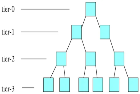
The multi-tier Data Grid architecture was first proposed by MONARC project [11], which aims to model the global distributed computing for the Large Hadron Collider (LHC) experiments [12], which produce roughly 15 Petabytes of data. CERN turned to grid computing to share the data with computer centers around the world. The Worldwide LHC Computing Grid (WLCG) is a distributed computing infrastructure arranged in tiers that can give a community of over 8000 physicists near real-time access to LHC data. The data that produced from these experiments will be distributed using a four-tier hierarchical Data Grid with CERN as the root( tier 0 site). A primary backup of raw data will be stored in tier-0. After initial processing, this data will be distributed to a series of regional tier-1 centers that will make data available to many national tier-2 centers. Individual scientists will access these data through tier-3 centers, which might consist of local clusters in a University Department. The hierarchical topology provides an efficient and cost-effective method for sharing data, computing and network resources. Network topology is shown in Figure 1.
tier-0
tier-1
tier-2
tier-3
Figure 1. Multi-tier Network Topology Architecture
To minimize data access time, work load and save the space of storage, replicas of the data might be created and spread from the root to regional, national, and/or institutional centers. In such a system, a user of a local site would try to locate a replica locally. If a replica was not present, the request would go to the parent node to find a replica there. Generally, a user request goes up the hierarchy and uses the first replica encountered along the path towards the root.
The data storage space in each layers gradually decreases, spacetier−0 > spacetier−1 > spacetier−2 > spacetier−3. The bandwidth between the layers gradually decreases, bandwidthtier−0>= bandwidthtier−1 >= bandwidthtier−2 >=bandwidthtier−3.
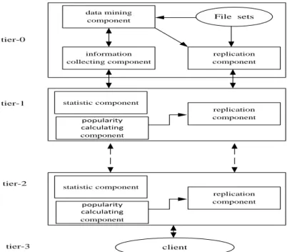
Root node has all of the data, it consists of three basic components: information collecting component, data mining component, replication component. The information collection components collected basic data access information from the lower tiers regularly, such as: the number of file access, file access time, the node that access to the file,the file access sequence of each node etc . The data mining components mainly used to analyze the file sequence to establish the correlation between the file and confidence. Confidence is a credible probability of the correlation between files. The Replication component mainly used for data replication, replication is based on the lower of the request and file popularity. The three cases will generate replication:
1) The lower nodes request data;
2) If the popularity of the file A exceeds a given threshold value, and the degree of confidence between the file A and the related file B is higher than the specified threshold value, then even if the file B's popularity does not reach the specified threshold, it will be copied to the lower node with A.
The middle layer nodes have three components: statistic component, popularity calculating component and replication component. Statistic component collects access number of data and sum from the lower layer. Popularity calculating component calculated the popularity of the file being accessed. Replication component sends replicating request to the upper or duplicate replicas to lower layer and replicates data to the lower tie. The system structure is as shown in Figure 2.
information collecting component data mining component replication component File sets client tier-0 tier-1 tier-2 statistic component replication component popularity calculating component statistic component replication component popularity calculating component tier-3
Figure 2. System Structure Diagram
4. Algorithm
4.1. Algorithm in Root Node
The algorithm takes into account spatial (file) locality and temporal (time) locality. It is based on the popularity and the concept of support and confidence. It finds out the correlation between the data files through data access number and data access serial. System prefetch frequently accessed files and their associated files to the location near the access site through the popularity of the files, thereby reducing the access time and saving space of storage. Support and confidence are the basic concepts of data mining association rules, which respectively showed the usefulness and certainty in data discovery rules.
Rule 1: A⇒B set up in transaction D, it has support s, s is percent of A∪B in transaction D, it is the P(A ∪ B) . So support is defined as:
support(A ⇒ B) = P(A ∪ B) (1)
Each discovery mode should be represented by an certainty measure of its effectiveness or reliability, so rule 2 is:
Rule 2: A⇒ B has confidence c, it is percent both A and B in transaction D. It is conditional probability P(A | B), so the certainty measure confidence is defined as :
confidence(A ⇒B) = P(A | B) (2)
If rule 1 and rule 2 meet the specified minimum support and confidence that the rules for strong association rules.
Rule 3: if support ≥ mini_support and confidence ≥ mini_confidence, it is strong association rule. (3) The mini_support is minimum support, and mini_confidence is minimum confidence. It needs the divided file access subsequence, before the support and confidence of data mining. The purpose of establishing access subsequence is to cut longer file access sequence, and save the time of statistics. It cuts window at a fixed length, and the tail less than the length of the window is filled with the empty. The algorithm may lead to less accessed data to be copied if you only consider the support and confidence in the data
grid. In order to select the appropriate data to replicate, the algorithm counts sum for each file accessed by the collecting file access times of child nodes, calculates the popularity of files. It prefetch files as close as possible to the end user through the support, confidence and popularity. In multi-tier data grid , each node belongs to a special tier. Tier (m) is the number of tie where node m is in. If a node m and n are directly connected, and tier(m)=tier(n)-1, so m is the parent of n which is child node. At each fixed time interval, the middle layer and the root node collects statistical information at the next layer nodes, and sum access numbers of the data file.
( ) q v a a v c h i l d q A c c e s s N u m A c c e s s N u m
(4)AccessNum present the access numbers of file a that is statistical in node q.
Root node collects information from tier-1 layer by the information collection component, finds out the file that access numbers exceeds the threshold and its associated file by data mining component, and then copy the files to the corresponding node in the intermediate layer. These files are those access numbers surpass threshold and related files those meet the corresponding support and confidence. The algorithm has two main sub-algorithms: data mining algorithm and replication algorithm.
4.1.1 Data Mining Algorithm: data mining component uses data mining algorithm to
find out file that needs replicate. Data mining is based Frequent Pattern(FP) growth algorithm. The algorithm is shown in Figure 3.
FP_tree ({file_serial}, mini_support) {
statistics file access numbers In accordance with the formula 1 If (AccessNum >= threshold )
{ {Support(a)} <- SORT-DEC(a, threshold) for a file serial } T <- Null
{[p|P] }<- Sort({file_serial}) based on {Support(a)} Tree <- insert_tree([p|P], T) Output( Tree ) insert_tree([p|P], T) If (N.name==p.name) N.count = N.count + 1 Else { N.count =1 T = parent(N) If (P ≠ Null) Call insert_tree([P], N) } FP-growth(Tree, x) { B = null If( only one path) B= B∪X
Support(B)= mini_support(B) Else
for( N child (Tree.root)) { B = N ∪ X
Support(B)= support(N) } TreeB <- FP_tree ({file_serial}, H) If TreeB ≠ null
Call FP-growth(TreeB, B)
Using the formula (1),(2) and (3) Get support(B) and confidence(B), AccessNum If (support(B) and confidence(B) meet rule 3)
Call replicate (File_serial, threshold) }
Figure 3. Data Mining Algorithms
The algorithm uses FP tree function to construct tree, and then finds out all of frequent sets through FP-growth, finally computing support, confidence and AccessNum. If support and confidence meet rule 3, then root node calls replication algorithm. FP tree is used to build FP tree. Its input value is file serial and minimum support. It first statistics numbers of file access for all of files in the first line. In 3-6 line, it sorts files in file serial in accordance with descending order, inserts the files into tree whose the root node is Null, and records the support at each node. Insert tree function is use to insert node in tree. FP-growth algorithm searches frequent sets from tree that is built by FP tree algorithm.
4.1.2 Replication Algorithm in root node: Replication components in root node mainly
replicate files. They replicate files through AccessNum, support and confidence. The AccessNum is access number of the file. They dynamically reselect the files that need to be copy when the 3 parameters change. So at the end of each time interval, the replication components check if any changes have occurred. The replication component have two cases: first, the root node send the file that is requesting to tier -1; second, when file’s
AccessNum becomes greater than threshold, if support and confidence satisfy the rule 3, file and its related file are replicated. Replication algorithm is shown in Figure 4.
replicate (File_serial, threshold) {
1 A <- Sort-Dec(a, threshold) for a file serial
2 If (a.support >= mini_support and a.confidence >= mini_confidence ) 3 AandRelate <- {a} ∪ {related files}
4 End if 5 receive(a) 6 if(a.AccessNum< threshold) 7 send(a) 8 else if 9 sent(AandRelate) 10 endif }
Figure 4. Replication Algorithm in Root Node
4.2. Algorithm in the Intermediate Layer
The middle layer nodes have three components: statistic component, popularity calculating component and replication component. The middle layer contains two main algorithms: popularity dynamically change algorithm and replication algorithm. The file popularity calculating component calculated files popularity in each time interval by popularity dynamically change algorithm. The replication components perform replication algorithm to request copying files, or copy the file to the lower to the upper layer.
4.2.1 Popularity dynamically change algorithm: popularity dynamically change
algorithm adjust popularity of the files real time. Each middle layer node dynamically replicates data based on popularity. Popularity adjustments consist of three parts: growth period, stable period and decay period. Growth period indicates that the file be accessed in each interval,, its popularity gradually increase. In the stable period the popularity of the data file remains unchanged. it showed that the file has not been accessed within the specified time. The decay period indicated that file is not accessed after a long time, its popularity gradually decreases. Where a and b are constants. The Popi(f) is popularity of the file f in phase i. The r
c
A is access times of file f.
( 1 ) ( 1 ) ( 1 ) ( ) ( ) ( ) * ( ) r i c i i i P o p f a A P o p f P o p f b P o p f (5)
4.2.2 Replication Algorithm in the Intermediate Layer: Replication algorithms in the
intermediate layer need to consider to sent request to the upper layer, store the replicas in the local limited storage space, but also copy the files to the lower layer according to the underlying replication request.
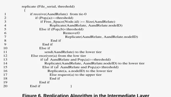
This algorithm is different from the algorithm of root node. It needs not only send request of replication to upper layer if the popularity of file is greater than threshold value, but also replicate files to lower tier. In order to copy files to an intermediate node, we need consider limited storage space in the intermediate layer node. Figure 6 is the replication algorithm in the intermediate layer algorithm pseudo-code.
replicate (File_serial, threshold) {
1 if receive(AandRelate) from tie-0 2 if (Popi(a)>=threshold)
3 if Free_Space(Node.id) >= Size(AandRelate) 4 Replicate(AandRelate, AandRelate.nodeID) 5 Else if (Popi(b)<threshold)
6 Remove©
7 Replicate(AandRelate, AandRelate.nodeID) 8 End if
9 End if 10 Else if
11 send(AandRelate) to the lower tier 12 Else receiver(a) from the low tier
13 if (aÎAandRelate and Popi(a)>=threshold)
14 Replicate(AandRelate, AandRelate.nodeID) to the lower tier 15 Else if (aÎAandRelate and Popi(a)<threshold)
16 Replicate(a, a.nodeID) to the lower tier 17 Else request(a) to the upper tier 18 End if
19 End if
20 End if }
Figure 6. Replication Algorithm in the Intermediate Layer
If the node of the intermediate layer receives the copy request of the lower nodes, it first check whether or not a copy of the data exists in the node, if it has the replica, it copies the replica to the lower node data, updates popularity of data access and access time; If the node does not have a copy of the data, the node sent replication request to the upper node (if any intermediate nodes do not have a copy of the data, finally the copy will be find in the root); When the node receives the copy of the data from the upper layer, it check whether the data popularity is greater threshold, a copy of the data will be replicated to the node if the file threshold meet the requirements, and the copy is passed to the lower node. When the copy is replicated in the node, the node first check whether the storage space of the node meets storage space requirements of the copy and the relevant files; if storage space is not enough, then delete some files. Node sorted files in ascending order that is based on the popularity of the file, then delete files that its popularity is less than the copy that need be replicated, until the space meet requirements. If the popularity of the file is the same, node delete the copy that its access time is earlier. After node replication is complete, node updates the file access time and the frequency of data access.
There is a data storage detection algorithm in replication component of the intermediate layer. It regularly detects the file popularity. If the popularity of the file is less than the specified threshold, then the algorithm delete the file to free up storage space.
5. Simulation Results
OptorSim is used as the simulation tool to evaluate the algorithm performance in data grid. It is a simulation toolkit written in JAVA language [13], used to simulate the actual data grid structure, and execute job scheduling and replication strategies at the structure.
Optorsim consists mainly of Resource Broker (RB) , Computing Elements (CEs) , Storage Elements (SEs) and Replica Manager (RM)[14] . In the simulation each CE is represented by a thread. Job submission to the CEs is managed by another thread; the RB ensures every CE continuously runs jobs by frequently attempting to distribute jobs to all the CEs. When the RB finds an idle CE, it selects a job to run on it according to the policy of the CE. The data files that jobs need is stored in Ses. Each site handles its file content with a RM, within which a Replica Optimiser (RO) contains the replication algorithm which drives automatic creation and deletion of replicas.
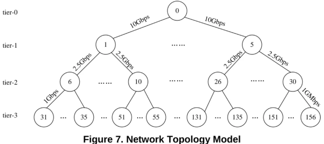
The simulated Data Grid architecture between the sites is adopted from the estimations for the CMS experiment [15]. The infrastructure has four tiers, Root node is tier-0; five regional centers are at tier-1; national centers is tier-2, where each regional centers has 5 national centers; and institute centers is tier-3 where each national centers has 5 institute centers. Tier-3 generates all data requests. The network bandwidth is 10Gbps between tier-0 and tier-1, and 2.5Gbps between tier-1 and tier-2, the bandwidth is 1Gbps between tier-2 and tier-3. The network topology model is shown in Figure 7.
156 151 135 131 55 51 35 31 6 10 26 30 1 5 0 …… …… …… …… … … … … tier-0 tier-1 tier-2 tier-3 10Gbps 2.5G bps 10Gb ps 2.5G bps 2.5Gbp s 2.5G bps 1Gbp s 1GM bps
Figure 7. Network Topology Model
There are 1,000,000 data files in the system. The size of files is 200TB. The data access requests follow Poisson arrival. The probability of requests for the nth most popular file chooses Geometric distribution, Zipf-like distribution. In Geometric distribution, the file request probability is P(n) = p(1 − p)n−1 , where n = 1, 2, ... and 0 < p < 1. The value of p takes 0.01 in experiment. In Zipf-like distribution [11], the number of requests for the nth most popular file is proportional to n−α, where α is a constant. Zipf-like distribution exists widely in the internet world. The value of α = 0.8 and α = 1 respectively in simulation. Root node stores all data files. Tier-1 and tier-2 have limited storage size, they storage configuration for simulation are shown in table 1. Tier-3 can cache files, its storage size is set as 2GB. The parameters values of Formula 5 are: The initial value of Pop is 0.5, the value of a takes 0.75, the value of b takes 2. The replication threshold is set to the average access counts of all the files stored. For example, the node P has k files which have been accessed a total of m times, so the replication threshold is m/k. Figure.6-Figure.8 show the average response times of different data access requests under different storage configurations. Storage configuration is measured by relative capacity ratio, which is defined as ratio of data file size and the total space in tier-1 and tier-2. The performance metrics of dynamic algorithm include the average response time. The average response time is the mean time that is time interval between request and receive files. The relative capacity ratio of the replica servers is defined as r=S/D, where S is the total storage size of the concerned replica servers and D is the total size of all data files in the Data Grid.
Table 1. Multi-tier Data Grid Storage Configuration
Case Tier-1 Tier-2 relative capacity ratio(%)
Node storage Size(T) Total Size(T) Node storage Size(T) Total Size(T) 1 20 20*5=100 5 5*25=125 (100+125)/200=112.5 2 10 10*5=50 2.5 2.5*25=62.5 (50+62.5)/200=56.25 3 5 5*5=25 1.25 1.25*25=31.25 (25+31.25)/200=28.125 4 2.5 2.5*5=7.5 0.625 0.625*25=15.625 (7.5+15.625)/200=11.5625 5 1 1*5=5 0.5 0.5*25=12.5 (5+12.5)/200=8.75
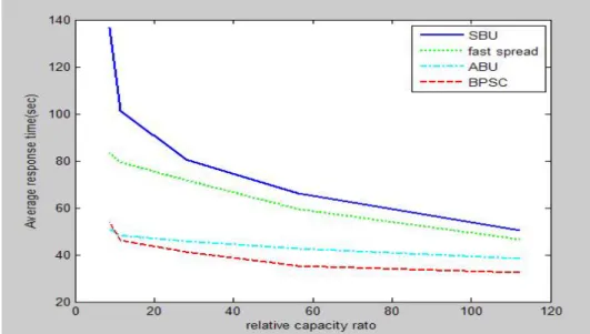
The simulation results for the Fast spread, SBU, ABU and BPSC in geometric distribution are shown in Figure 8.
Figure 8. Average Response Time for Geometric Distribution-0.01
In geometric distribution, SBU algorithm has a larger average response time in the lower storage configuration. The average response time of the SBU algorithm is superior to fast spread following the increase in the storage configuration. BPSC are better than ABU, SBU and fast spead. The average response time of BPSC is worse than ABU in the lowest storage configuration. This is because BPSC need delete some files to free up space.
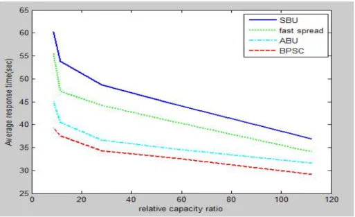
The Zipf-like with α = 0.8 is called Zipf-0.8 (Figure 9). The average response time of SBU is higher than fast Spread, ABU and BPSC. When the relative capacity is lower, fast spread is superior to ABU and BPSC. ABU and BPSC are better than fast spread when the relative capacity increases. BPSC’s average response time is slightly smaller than ABU. This is because the file’s accessed frequency is increase in Zipf-0.8, BPSC can quickly find files and related data.
For Zipf-1.0 (Figure 10), ABU outperforms Fast Spread and SBU. SBU’s average response time is highest in the four algorithms, and BPSC has lowest average response time. The average response time of BPSC is slightly lower 10.1% than ABU. This is because that the files accessed by the clients are concentrated in a smaller range for Zipf-1.0, so the frequently accessed files and related files can be mined quickly by BPSC.
Figure 10. Average Response Time for Zipf-like 1.0
6. Conclusion
In this paper, dynamic replication algorithm BPSC is presented for the multi-tier Data Grid. The algorithm takes into account spatial (file) locality and temporal (time) locality. BPSC identifies frequently accessed files and their associated files based on the number of file access, support and confidence. It adjusts popularity of files in real-time, dynamically copy the data to the middle layer nodes, greatly reducing the average response time data. The algorithm is simulated by Optorsim, and compared with the fast spread, SBU, ABU algorithm. The simulation results demonstrate that BPSC dynamic replication algorithm can has a shorter performance.
Acknowledgements
This paper is supported by the National Natural Science Foundation of China (No. 61173020), and the National High Technology Research and Development Program of China(863 Program, 2013AA01A215).
References
[1] K. Ranganathan and I. Foster, “Design and Evaluation of Dynamic Replication Strategies for a High Performance Data Grid”, Proc. Intl. Conf. on Comp. in High Energy and Nuclear Physics, (2001). [2] K. Ranganathan and I. T. Foster, “Identifying Dynamic Replication Strategies for a High Performance
Data Grid”, Proc. 2nd Intl. Wksp. on Grid Computing, (2001), pp. 75–86.
[3] M. Tang, B. S. Lee, C. K. Yao and X. Y. Tang, “Dynamic replication algorithm for the multi tier data grid”, Future Generation Computer Systems, vol. 21, no. 5, (2005), pp. 775-790.
[4] Y. Lin, P. Liu and J. Wu, “Optimal Placement of Replicas in Data Grid Environments with Locality Assurance”, Proc. 12th Intl. Conf. on Parallel and Distributed Systems, vol. 01, (2006), pp. 465–474. [5] L. M. Khanli, A. Isazadeh and T. N. Shishavanc, “PHFS: a dynamic replication method to decrease
access latency inmulti tier data grid”, Future Generation Computer Systems, vol. 27, (2010), pp. 233– 244.
[6] R. S. Chang and H. P. Chang, “A dynamic data replication strategy using access weights in data grids”, The Journal of Supercomputing, vol. 45, no. 3, (2008), pp. 277–295.
[7] N. Mansouri and G. Hosein Dastghaibyfard, “Enhanced Dynamic Hierarchical Replication and Weighted Scheduling Strategy in Data Grid”, Journal of Parallel and Distributed Computing, vol. 73, no. 4, (2013) April, pp. 534-543.
[8] N. Saadat and A. Masoud Rahmani, “PDDRA: A new pre-fetching based dynamic data replication algorithm in data grids”, Future Generation Computer Systems, vol. 28, no. 4, (2012) April, pp. 666-681. [9] T. Ma, Q. Yan, W. Tian, D. Guan and S. Lee, “Replica creation strategy based on quantum evolutionary
algorithm in data gird”, Knowledge-Based Systems, vol. 42, (2013) April, pp. 85-96.
[10] E. Kayaaslan, B. Barla Cambazoglu and C. Aykanat, “Document replication strategies for geographically distributed web search engines”, Information Processing & Management, vol. 49, no. 1,
(2013) January, pp. 51-66.
[11] http://monarc.web.cern.ch/MONARC/. [12] http://home.web.cern.ch/about/computing.
[13] D. G. Cameron, R. Schiafino, J. Ferguson, A. P. Millar, C. Nicholson, K. Stockinger and F. Zini, OptorSim v2.1 Installation and User Guide, (2006) October.
[14] Optorsim: A Simulation Tool for Scheduling and Replica Optimisation in Data Grids.
[15] K. Holtman, “CMS Data Grid system overview and requirements”, CMS Experiment Note 2001/037, CERN, Switzerland, (2001).
Authors
Zhongqiang Cui
,
received his B.S. and M.S. degrees in computer science from the YanShan University, PR China, in 2000 and 2005, respectively. Since 2009 he has been a Ph.D. candidate at the Harbin Institute of Technology. His research interests include fault-tolerant computing, data grid and distributed system.De-Cheng Zuo, received the Ph.D degree in computer systems
from the Harbin Institute of Technology, PR China, in 2001. He is a professor of the School of Computer Science and Technology at the Harbin Institute of Technology. His main research interests are fault-tolerant computing and mobile computing.
Zhan Zhang, received his B.S., M.S. and Ph.D degrees in
computer science from the Harbin Institute of Technology, PR China, in 2001, 2003 and 2007, respectively. He is a professor of the School of Computer Science and Technology at the Harbin Institute of Technology. His research interests include fault-tolerant computing and mobile computing