Optimal column layout for hybrid workloads

Boston University

OpenBU

http://open.bu.edu

Computer Science BU Open Access Articles

2019-09-01

Optimal column layout for hybrid

workloads

This work was made openly accessible by BU Faculty. Please

share

how this access benefits you.

Your story matters.

Version

Published version

Citation (published version): Manoussos Athanassoulis, Kenneth Bøgh, Stratos Idreos. 2019.

"Optimal Column Layout for Hybrid Workloads." Proceedings of the

VLDB Endowment, Volume 12, Issue 13, pp. 2393 - 2407.

https://doi.org/10.14778/3358701.3358707

https://hdl.handle.net/2144/40617

Optimal Column Layout for Hybrid Workloads

Manos Athanassoulis

[email protected]

Kenneth S. Bøgh

[email protected]

Stratos Idreos

[email protected]

ABSTRACT

Data-intensive analytical applications need to support both efficient reads and writes. However, what is usually a good data layout for an update-heavy workload, is not well-suited for a read-mostly one and vice versa. Modern analytical data systems rely on columnar layouts and employ delta stores to inject new data and updates.

We show that for hybrid workloads we can achieve close to one order of magnitude better performance by tailoring the column lay-out design to the data and query workload. Our approach navigates the possible design space of the physical layout: it organizes each column’s data by determining the number of partitions, their corre-sponding sizes and ranges, and the amount of buffer space and how it is allocated. We frame these design decisions as an optimiza-tion problem that, given workload knowledge and performance re-quirements, provides an optimal physical layout for the workload at hand. To evaluate this work, we build an in-memory storage en-gine, Casper, and we show that it outperforms state-of-the-art data layouts of analytical systems for hybrid workloads. Casper deliv-ers up to 2.32×higher throughput for update-intensive workloads and up to 2.14×higher throughput for hybrid workloads. We fur-ther show how to make data layout decisions robust to workload variation by carefully selecting the input of the optimization. PVLDB Reference Format:

Manos Athanassoulis, Kenneth S. Bøgh, Stratos Idreos. Optimal Column Layout for Hybrid Workloads.PVLDB, 12(13): 2393-2407, 2019. DOI: https://doi.org/10.14778/3358701.3358707

1.

INTRODUCTION

Modern data analytics systems primarily employ columnar stor-age because of its benefits when it comes to evaluating read-heavy analytic workloads [1]. Examples include both applications and systems that range from relational systems to big data applications like Vertica [48], Actian Vector (formerly Vectorwise [84]), Oracle [47], IBM DB2 [17], MS SQL Server [51], Snowflake [30], and in the Apache Ecosystem, the Apache Parquet [9] data storage format. ∗_{Part of this work was done while the author was a postdoctoral researcher} at Harvard University.

†_{Work done while the author was a visiting student at Harvard University.}

This work is licensed under the Creative Commons Attribution-NonCommercial-NoDerivatives 4.0 International License. To view a copy of this license, visit http://creativecommons.org/licenses/by-nc-nd/4.0/. For any use beyond those covered by this license, obtain permission by emailing [email protected]. Copyright is held by the owner/author(s). Publication rights licensed to the VLDB Endowment.

Proceedings of the VLDB Endowment,Vol. 12, No. 13

ISSN 2150-8097. DOI: https://doi.org/10.14778/3358701.3358707 0 200 400 600 800 1000 1200 0 50 100 150 200 250

optimal column layout

(Casper) col-store with delta(state-of-art) vanilla column-store(baseline)

Th rou ghput (op/s ) La te ncy ( ms)

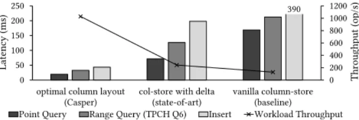
Point Query Range Query (TPCH Q6) Insert Workload Throughput 390

Figure 1: Existing analytical systems have 2×higher perfor-mance than vanilla column-stores on hybrid workloads by uti-lizing a delta-store. Using a workload-tailored optimal column layout, Casper brings an additional 4×performance benefit. The HTAP Evolution.Analytical applications are quickly transi-tioning from read-mostly workloads to hybrid workloads where a substantial amount of write operations also needs to be supported efficiently. These hybrid transactional analytical workloads (HTAP) typically target state-of-the-art analytics, while still supporting ef-ficient data ingestion [62, 66]. New designs targeting HTAP work-loads are coming both from academic research projects [10, 11, 45, 49, 54, 58, 64, 67] and commercial products like SAP Hana [33, 68, 77], Oracle [61], Microsoft SQL Server [50], and MemSQL [76].

The Problem: Conflicting Design Goals for HTAP.One big chal-lenge when designing systems for HTAP workloads comes from the fact that data layout decisions designed for read-intensive sce-narios do not typically work well for write-intensive scesce-narios and vice versa. Finding the optimal layout can give a massive perfor-mance benefit, however, existing data systems come with a fixed design for many core data layout decisions. This means that they are locked into a specific behavior and are unable to approach the theoretical optimal, thus, missing out on significant benefits.

The Solution: Learning Column Layouts. Our insight is that there are certain design choices for which we should not be mak-ing a fixeda prioridecision. Instead, we can learn their optimal tuning to efficiently support HTAP workloads with a single copy of the data. In modern analytical systems there is a set of decisions that always makes sense. For example, nearly all systems choose to store columns as fixed-width arrays, which helps with hardware-conscious optimizations, like vectorization, SIMD processing, and compression. Other decisions are typically fixed, though in prac-tice, the optimal choice depends on the workload. In particular, in this paper, we focus on three prominent design decisions: (i) how to physically order data [40, 78], (ii) whether columns should be dense, and (iii) how to allocate buffer space for updates (e.g., delta-store [38, 48] and ghost values [18, 19, 44]). We show that systems should be tunable along those decisions for a given application, and we demonstrate how to do this in an optimal and robust way.

Example. Figure 1 shows the performance of a workload with both transactional (point queries and TPC-H updates) and

analyti-cal (TPC-H Q6) access patterns, when executed using three differ-ent approaches: base column-stores (without any write optimiza-tions), state-of-the-art columnar layouts with a delta store, and a workload-tailored optimal column layout proposed by our system, Casper. We implemented all approaches in a state-of-the-art column-store system that exploits parallelism (using all 32 cores). Our implementation supports fast scans that employ tightforloops, multi-core execution, and work over compressed data.

The state-of-the-art approach, which sorts the queried columns and maintains a delta-store, leads to a 1.9×increase in throughput when compared to the baseline column-store. In comparison, the optimal layout determined by Casper leads to 8×improvement in overall performance. Casper’s physical design decisions combine fine-grained partitioning with modest space for update buffering (1% of the data size in this experiment) which is distributed per partition (details for the partitioning process in §4 and §5).

Challenge 1: Fast Layout Discovery. The fact that we can see massive improvements when we tailor the layout of a system to the access patterns is not by itself surprising. There are several challenges though. First, finding this optimal layout is expensive: in the worst case, an exponential number of data layout strategies needs to be enumerated and evaluated.

To be able to make fast decisions, we formulate the data lay-out problem as a binary optimization problem and we solve it with an off-the-shelf solver [8]. We keep the optimization time low by dividing the problem into smaller sub-problems. We exploit that columns are physically stored in column chunks, and we partition each chunk independently, thus reducing the overall complexity by several orders of magnitude (§6.3).

Challenge 2: Workload Tailoring. Second, we rely on having a representative workload sample. We analyze this sample to quan-tify the access frequency and the access type for each part of the dataset. As part of our analysis, we maintain workload access pattern statistics for both read operations (point queries and range queries) and write operations (inserts, deletes, and updates).

The column layouts can be tailored along many dimensions. The design space covers unordered columns to fully sorted columns, along with everything in between; that is, columns partitioned in arbitrary ways. We also consider the update policy and ghost val-ues, which balance reads and writes with respect to their memory amplification [15]. Ghost values are empty slots in an otherwise dense column, creating a per-partition buffer space. Our data lay-out scheme creates partitions of variable length to match the given workload: short granular partitions for frequently read data, large partitions to avoid data movement in frequently updated ranges, while striking a balance when reads and updates compete.

Challenge 3: Robustness.Third, when tailoring a layout to a given workload, there is the chance of overfitting. In practice, workload knowledge may be inaccurate and for dynamic applications may vary with time. A system with a layout that works perfectly for one scenario may suffer in light of workload uncertainty. We show that we can tailor the layout for a workload without losing performance up to a level of uncertainty.

Positioning. We focus on analytical applications with relatively stable workloads which implies that a workload sample is possible to achieve. For example, this is the case for most analytical appli-cations that provide a regular dashboard report. In this case, our tool analyzes the expected workload and prepares the desired data layout offline, similar to index advisors in modern systems [3, 83]. For more dynamic applications with unpredictable workloads, an adaptive solution is more appropriate. Our techniques can be extended for such dynamic settings as well, by periodically

analyz-Norm. Latency Read Cost Write Cost Nor m. Late ncy Read Cost Write Cost

# non-overlapping partitions memory amplification

(a) Impact of structure (b) Impact of ghost values

Figure 2: Accessing a column is heavily affected by the struc-ture of the column (e.g., sorted, partitioned). Read cost (a) log-arithmically decreases by adding structure (partitions), while using ghost values to expand the column layout design space (b) reduces write cost linearly w.r.t. memory amplification.

ing the workload online (similar to how offline indexing techniques were repurposed for online indexing [24]) and reapplying the new format if the expected benefit crosses a desired threshold.

Contributions.Our contributions are summarized below: • We describe the design space of column layouts containing

par-titioning, update policy, and buffer space (§2), a rich design space that supports a diverse set of workloads.

• We introduce (i) theFrequency Modelthat overlays access pat-terns on the data distribution (§4.2); (ii) a detailed cost model of operations over partitioned columns (§4.4); and (iii) an alloca-tion mechanism for ghost values (§4.6).

• We formalize the column layout problem as a workload-driven, binary integer optimization problem that balances read and up-date performance, supports service-level agreements (SLAs) as constraints, and offers robust performance even when the train-ing and the actual workloads are not a perfect match (§5). • We integrate the proposed column layout strategies in our

stor-age engine Casper (§6). We show that Casper finds the optimal data layout quickly (§6.3), and that it provides up to 2.3× per-formance improvement over state-of-the-art layouts (§7).

2.

COLUMN LAYOUT DESIGN SPACE

In this section, we define the problem and the scope of the pro-posed approach. State-of-the-art analytical storage engines, store columns either sorted based on a sort key (i.e., one of the columns), or following insertion order. On the other hand updates are usually applied out-of-place using a global buffer [1, 39, 48, 84]. Casper explores a richer design space that (i) uses range partitioning as an additional data organization scheme, (ii) supports in-place, out-of-place, and hybrid updates, and (iii) supports eitherno,global, or per-partitionbuffering as shown in Table 1. By considering a wider design space, we allow for further performance optimizations with-out discarding the key design principles of analytical engines that benefit hybrid analytical workloads.

Table 1: Design space of column layouts. Data Organization Update Policy Buffering

(a) insertion order (a) in-place (a) none

(b) sorted (b) out-of-place (b) global

(c) partitioned (c) hybrid (c) per-partition

Scope of the Solution. Casper targets applications with a hybrid transactional analytical nature, with an arbitrary yet static workload profile. Casper uses this workload knowledge to find a custom-tailored column layout that outperforms the state of the art.

Horizontal Partitioning vs. Vertical Partitioning. Casper’s de-sign space includes the traditional global buffering approach of write-stores [78] and operates orthogonally to schemes that em-ploy arbitrary vertical partitioning (e.g., tiles [11]). As a result, our

3 1 2 4 8 7 5 15 19 20 55 32 23 65 67 125 82 71 3 1 2 4 8 7 5 15 19 20 55 32 23 65 67 125 82 71 3 1 2 4 8 7 5 15 19 20 55 32 23 65 67 125 82 71

(a) A range partitioned column. (b) Looking for value 15. (c) Looking for values in[6,43).

Figure 3: Maintaining range partitions in a column chunk allows for fast execution of read queries. For point queries (b), the partition that may contain the value in question is fully scanned. For range queries (c) the partitions that (may) contain the first and the last element belonging to the range are scanned, while any intermediate partitions are blindly consumed.

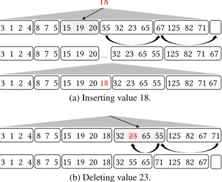
18

3 1 2 4 8 7 5 15 19 20 __ 32 23 65 55 125 82 71 67

3 1 2 4 8 7 5 15 19 20 55 32 23 65 67 125 82 71

3 1 2 4 8 7 5 15 19 20 18 32 23 65 55 125 82 71 67

(a) Inserting value 18.

3 1 2 4 8 7 5 15 19 20 18 32 55 65 71 125 82 67

3 1 2 4 8 7 5 15 19 20 18 32 23 65 55 125 82 67 71

(b) Deleting value 23.

Figure 4: Inserting and deleting data in a partitioned column chunk uses rippling and restricts data movement.

column layout strategies can also be used for tables with tiles or projections [78]. In the case of projections, the read workload is distributed amongst the different projections. As a result, the col-umn layout can be further tailored for each projection leading to potentially greater benefits.

Partitioning as an Update Tuning Knob.The core intuition about why range partitioning can work as a way to balance read and write costs is twofold: read queries with small selectivity favor high num-ber of partitions (more structure) because then they will only read the relevant data, while updates, insert, and deletes, favor a low number of partitions (less structure) because each such operation can operate by moving data across partition boundaries. With re-spect to read-only workloads, different partitioning strategies have different impact. If a workload has different access patterns in dif-ferent parts of the domain, equi-width partitioning can lead to un-necessary reads. Narrow partitions are needed for the parts of the data that correspond to point queries, or to the beginning/end of range queries. On the other hand, for the part of the domain which is less frequently queried, coarser partitioning is enough.

The impact of adding structure to the data on the read and write costs is conceptually shown in Figure 2a. For example, when a column chunk withMCelements is partitioned inkpartitions, the

estimated cost of a point query is on average the cost of readingMC k

elements, assuming equi-width partitions. On the other hand, the cost of inserts (and deletes) is on averagek/2. Hence, the num-ber of partitionsk is an explicit tuning knob between read and update performance. Ideally, however, a locally optimized parti-tioning scheme would allow a workload with skewed accesses in different parts of the domain to achieve optimal latency.

Ghost Values. Delete, insert, and update approaches require data movement that can be reduced if we relax the requirement to have the whole column contiguous. Allowing deletes to introduce empty slots in a partition results in a delete operation that only needs to find the right partition and flag the value as deleted. To better op-timize for future usage, the empty slot is moved to the end of the partition to be easily consumed when an insert arrives, or when a

3 1 2 4 _ 8 7 5 _ _ 15 19 20 18 32 55 65 _ _ 125 82 67 71 _ _

Figure 5: Adding ghost values allows for less data movement; inserts use empty slots and deletes create new ones.

neighboring partition needs to facilitate an insert and has no empty slots of its own. These empty slots, calledghost values, require extra bookkeeping but allow for a versatile and easy-to-update par-titioned column layout with per-partition buffering. Ghost values expand the design space by reducing the update cost at the expense of increased memory usage, trading space amplification for update performance [14, 15].

Workload-Driven Decisions. Employing range partitioning and ghost values allows Casper to have a tunable performance that can accurately capture the requirements of hybrid workloads. Casper adjusts the granularity of partitions and the buffer space to navi-gate different performance profiles. In particular, by increasing the number of partitions, we achieve logarithmically lower read cost at the expense of a linear increase of write cost (Fig. 2a), and by increasing the buffer space, we achieve linearly lower write cost at the expense of a sublinear read performance penalty (Fig. 2b). Contrary to the previous workload-driven approaches, Casper does not care only for what types of operations are executed and at what frequency. Rather, it takes into account theaccess pattern distri-bution with respect to the data domain, hence making fine-grained workload-driven partitioning decisions. Overall, Casper collects detailed information about the access distribution of each opera-tion in the form of histograms with variable granularity and uses it to inform the cost models that we develop in the following sections.

3.

ACCESSING PARTITIONED COLUMNS

In this section, we describe Casper’s standard repertoire of stor-age engine operations. We further provide the necessary back-ground on operating over partitioned columns, as well as the build-ing blocks needed to develop the intuition about how to use parti-tioning for balancing read and write performance. Casper supports the fundamental access patterns of point queries, range queries, deletes, inserts, and updates [57]. For the following discussion, we assume a partition schemePwithkpartitions of variable size. A fixed-cost light-weight partition index is also kept in the form of a shallow k-ary tree (Fig. 3a).

Point Queries. The partition index provides the partition ID, and then the entire partition is fully consumed with a tightforloop scan to verify which data items of the partition qualify, as shown in Figure 3b. The cost of the query is given by the shallow index probe and the scan of the partition. Once the corresponding values are verified the query returns the positions of the qualifying values or directly the values (depending on the API of the select operator) to be consumed by the remaining operators of the query plan.

Range Queries. Similarly to point queries, a range query over partitioned data needs to probe the shallow index to find the first and the last partitions of the query result (Fig. 3c). The first and the last partitions are filtered, while the rest of the partitions are accessed when the result is materialized and can simply be copied to the next query operator as we know that all values qualify.

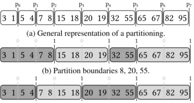
3 1 5 4 7 8 15 18 20 19 32 55 65 67 82 95

p0 p1 p2 p3 p4 p5 p6 p7

(a) General representation of a partitioning.

0 0 1 0 1 1 0 1

3 1 5 4 7 8 15 18 20 19 32 55 65 67 82 95

3 1 5 4 7 8 15 18 20 19 32 55 65 67 82 95

Figure 6: Representing different partitioning schemes (b) and (c) with block sizeB=2.

Inserts.An insert to a range partitioned column chunk can be ex-ecuted using the ripple-insert algorithm [41] causingO(k)data ac-cesses (Fig. 4a). When a value needs to be inserted in a partition, the ripple-insert brings an empty slot from the end of the column to that partition. Starting from the last partition, it moves the first element of each partition to the beginning of the next partition. The first movement happens between the first element of the last par-tition and the (already) available empty slot at the end of the col-umn. If no empty slots are available, the column is expanded. Then, starting from the last partition and moving toward the partition tar-geted by the insert, the first elements of consecutive partitions are swapped, in order to create an empty slot right after the end of the partition receiving the insert. The new value is inserted there and the partition boundaries of all trailing partitions are moved by one position. When inserting in themth partition the overall cost is (k−m), and, if data is uniform,k/2 on average.

Deletes. When a value (or row ID) to delete is received, the first step is to identify the partition that may hold this value using the shallow index. The next step is to identify the value or values to be deleted and move them to the end of the partition. Then, following the inverse of the previous process, the empty slots are moved to-wards the end of the column, where they can remain as empty slots for future usage. The data movement is now(k−m)·del card, wheremis the partition to delete from, anddel cardis the number of values that qualified for deletion.

Updates. An update is handled as a delete followed by an insert. This approach is followed in state-of-the-art systems and allows for code re-use. Alternatively, the shallow index is probed twice to find the source (update from) and the destination (update to) partitions, followed by a direct ripple update between these two partitions.

4.

MODELING COLUMN LAYOUTS

In this section, we provide the necessary modeling tools to view the column layout decision as an optimization problem, which cap-tures the workload access patterns and the impact of ghost values. We model the operations over partitioned columns with ghost val-ues (§4) and we show how to find the optimal column layout (§5).

Problem Setup.Each of the five operations may have an arbitrary frequency and access skew. In this general case, the ideal column layout forms partitions that minimize the overall workload latency, taking into account that each operation is affected differently from layout decisions. For ease of presentation, we first build a model without ghost values, incorporating them later on.

We formalize this as an optimization problem, where we want to find the partitioning schemePthat minimizes the overall cost of executing a workloadWover a datasetD:

arg minP cost(W,D,P) (1)

This formulation takes into account both the dataset and a sam-ple workload and aims to provide as output the ideal partitioning. It does so by first combining the distribution of the values of the domain with the distribution of the access patterns of the workload to form theeffective access distribution, by overlaying the access patterns on the data distribution. In order to formalize this problem accurately, we first need to define a way to represent an arbitrary partitioning scheme (§4.1), and subsequently, a way to overlay on it the representation of an arbitrary workload (§4.2). Next, we present a detailed cost model for each workload operation (§4.4). Finally, we consider how to allocate ghost values (§4.6).

4.1

Representing a Partitioning Scheme

We represent a partitioning scheme by identifying the positions of values that mark a partition boundary using a bit vector. In gen-eral, we can have as many partitions as the number of values in the column, however, there is no practical gain in having partitions smaller than a cache-line for main-memory processing. In fact, having a block size of several cache-lines is often more preferable because it naturally supports locality and sequential access perfor-mance. Note that duplicate values should be in the same partition.

A column is organized intoNbequally-sized blocks. The size of

each block is decided in conjunction with the chunk size to guaran-tee that the partitioning problem is feasible (more in §6.3). We rep-resent a partitioning scheme byNbBoolean variables{pi,fori=

0,1, ...,Nb−1}. Each variablepiis set to one when blockiserves

as a partition boundary, i.e., a partition ends at the end of this block. Note that the first block is beforep0. The exact block size is tun-able to any multiple of cache-line size, and affects the level of the detail of the final partitioning we provide. The smaller meaningful value is a cache-line, but in practice, a much coarser level of granu-larity is sufficient. Figure 6a shows an example dataset with blocks of size two and eight Boolean variables{p0, ...,p7}. Figures 6b and 6c show two different partitioning schemes. In Figure 6b, the first partition is three blocks wide, the second spans two blocks, the third is a single block, and the fourth spans two blocks. Figure 6c shows another partitioning scheme with four partitions, each one two blocks wide. This scheme captures any partitioning strategy, at the granularity of the block size or any coarser granularity chosen.

4.2

The Frequency Model

We now present a new access pattern representation scheme on top of the partitioning scheme of the previous section. The accessed data is organized in logical blocks (like in Figure 6) and the access patterns of each operation per block are documented. The size of a logical block is tunable, which allows for a variable resolution of access patterns, which, in turn, controls the partitioning overhead. The basic access patterns are produced by the five operations, how-ever, each one causes different types of accesses. Next, we describe in detail the information captured from a sample workload.

Given a representative sample workload and a column split into its blocks we capture which blocks are accessed and by which oper-ation, forming a set of histograms. We refer to this set of histograms as theFrequency Model(FM) because it stores the frequency of ac-cessing each part of the domain, which translates to access patterns in the physical layer.FMcaptures the accesses on the blocks, while the common cost to locate a partition is not kept as it is shared for each operation. The overall idea is that we capture accesses to each individual column block, in order to synthesize these blocks into partitions in a way that maximizes performance for the specific ef-fective access distribution.

While we model five general operations (point, and range queries, deletes, inserts, and updates), the different ways of accessing each

p0 p1 p2 p3 p4 p5 p6 p7

pq0:0 pq1:1 pq2:0 pq3:0 pq4:0 pq5:0 pq6:0 pq7:0

3 1 5 4 7 8 15 18 20 19 32 55 65 67 82 95

(a) PQ looking for value 4.

p0 p1 p2 p3 p4 p5 p6 p7

rs0:0 rs1:1 rs2:0 rs3:0 rs4:0 rs5:0 rs6:0 rs7:0

sc0:0 sc1:0 sc2:1 sc3:1 sc4:0 sc5:0 sc6:0 sc7:0

re0:0 re1:0 re2:0 re3:0 re4:1 re5:0 re6:0 re7:0

3 1 5 4 7 8 15 18 20 19 32 55 65 67 82 95

(b) RQ looking for range 4 to 19.

p0 p1 p2 p3 p4 p5 p6 p7

rs0:1 rs1:1 rs2:0 rs3:0 rs4:0 rs5:0 rs6:0 rs7:0

sc0:0 sc1:1 sc2:2 sc3:2 sc4:1 sc5:1 sc6:0 sc7:0

re0:0 re1:0 re2:0 re3:0 re4:1 re5:0 re6:1 re7:0

3 1 5 4 7 8 15 18 20 19 32 55 65 67 82 95

(c) RQ looking for range 2 to 66.

p0 p1 p2 p3 p4 p5 p6 p7 de0:0 de1:0 de2:0 de3:0 de4:0 de5:1 de6:0 de7:0

3 1 5 4 7 8 15 18 20 19 32 55 65 67 82 95

3 1 5 4 7 8 15 18 20 19 32 55 65 67 82 95

(e) Inserting value 16.

p0 p1 p2 p3 p4 p5 p6 p7

udf0:1 udf1:0 udf2:0 udf3:0 udf4:0 udf5:0 udf6:0 udf7:0

utf0:0 utf1:0 utf2:0 utf3:1 utf4:0 utf5:0 utf6:0 utf7:0

3 1 5 4 7 8 15 18 20 19 32 55 65 67 82 95

(f) Updating 3 to 16.

p0 p1 p2 p3 p4 p5 p6 p7

udb0:0 udb1:0 udb2:0 udb3:0 udb4:0 udb5:1 udb6:0 udb7:0

utb0:0 utb1:0 utb2:0 utb3:1 utb4:0 utb5:0 utb6:0 utb7:0

3 1 5 4 7 8 15 18 20 19 32 55 65 67 82 95

(g) Updating 55 to 17.

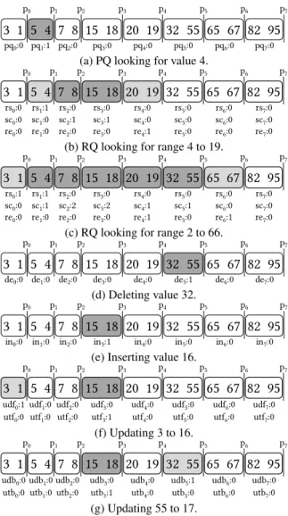
Figure 7: Frequency model in action. Here we show for each operation which partitions are accessed, and consequently, which histogram buckets are updated.

block are, in fact, more complex.FMutilizes ten histograms, each storing the frequency of a different sub-operation: (i) pqcounts block accesses for eachpoint query, (ii)rscounts block accesses for eachrange query start, (iii)recounts block accesses for each

range query end, (iv)sc counts full blockscansfor each range

query, (v)decountsdeletesfor each block, (vi)incountsinserts to each block, (vii)udf and (viii)udbstore when a block contains a value toupdate fromand it generates aforward/backwardripple, and, (ix)utf and (x)utbstoreswhen a block contains a value to update toand it generates aforward/backwardripple.

Update operations are captured by a set of four histograms to ac-count for the possible ripple action between the block we update from and the block we update into. In addition, we differentiate a forward ripple from a backward ripple to account for subtle model-ing details (discussed in §4.4). Each of the ten histograms contains a counter per block to reflect the respective accesses to this block, i.e., each bin of the histogram corresponds to a block. When calcu-lating the histograms from a sample workload, we do not actually materialize the results or modify the data; instead, we capture the access patterns as if each operation is executed on the initial dataset.

Example.We now explain how the histograms are populated using a series of examples in Figure 7. A point query touches a single block, which increments the relevant bin of thepqhistogram. For

Workload Sample

(a) (b)

Figure 8: LearningFMfrom (a) samples or (b) distributions.

example a point query for value 4 would be simulated by incre-mentingpq1(Fig. 7a). In the general case, a range query touches several blocks. In particular, one access is documented for the first block of the range atrs, one access for the last block of the range atre, and one access for each block between the two increasing the value of thescbins of the intermediate blocks. For example, a query looking for values 4≤v≤19 will incrementrs1,sc2,sc3, and re4, because the range query starts in block #1, scans block #2 and block #3, and finishes in block #4 (Fig. 7b). When another range query is documented, the buckets that are accessed by both will be further incremented (Fig. 7c). For each delete operation, thedehistogram corresponding to the block that contains the value to be deleted is incremented. Thus, the deletion of the value 32 incrementsde5(Fig. 7d). Inserts increment theinhistogram cor-responding to the block that the value would be inserted to. For example, inserting 16 in the previous example results in increment-ingin3(Fig. 7e). Finally, updates incrementudf for the old value andutf for the new value, orudbandutbrespectively. The choice depends on the relationship of the old value with the new value. If the new value islarger, thenudfandutfare incremented, and when the new value issmaller,udbandutbare incremented. For exam-ple, updating the value 3 to be 16 results in incrementingudf0and utf3(Fig. 7f). Similarly, updating 55 to 17 results in incrementing udb5andutb3(Fig. 7f).

The Frequency Model is built once all operations of the sample workload have contributed to the bins of the ten histograms. The ten histograms are represented by ten vectors. Thersibins form the

vector−RS→={rs0,rs1, . . . ,rsN−1}, and similarly, the vectors −→ RE, −→

SC,−→PQ,−→DE,−IN→,U DF−−−→,−U T F−−→,U DB−−→, andU T B−−→represent the cor-responding histograms. Using these vectors we build a cost-model that provides the cost of each operation for partitions of arbitrary size (multiple of block size) in §4.4.

Columns and Column-Groups.For ease of presentation our run-ning examples depict only one column, however, the same analysis can be directly applied to groups of columns since the Frequency Model is oblivious to whether each data item consists of a single value or multiple. Thus, the Frequency Model can generate the ef-fective access patternof a workload over a table resulting in multi-dimensional dynamic range partitioning. Once the workload access patterns are documented, any further decisions are taken based on the Frequency Model alone. We collect information on a per block basis regardless of the contents of the block.

4.3

Learning the

from Access Patterns

The previous discussion assumes that the Frequency Model uses a sample workload to estimate the histograms of each operations as shown in Figure 8a. The Frequency Model, however, can also use statistical knowledge of the workload access patterns to create access distribution histograms with the desired granularity. Having estimated the distribution of the access pattern of each operation as well as the data distribution, we can efficiently construct a his-togram with variable number of buckets as shown in Figure 8b. By default, each bucket corresponds to a memory block, however, this parameter is tunable. Finer granularity leads to better performance, at the cost of longer optimization runtime, and vice versa. In addi-tion, Casper can combine the two approaches and benefit from the recent advancements in learning data distributions from the work-load [46], and estimate online the access pattern distributions dur-ing normal operation.

4.4

Cost Functions

Now we model the cost of each access operation. Assuming

a dataset withM values, and using block sizeB we have up to

N=dM

Bepartitions. We assume that every partitioning scheme can

support up toN partitions, which in practice, depends onM and can be controlled by choosingB. We assume that accessing blocks comes at a cost following a standard I/O model where we have four main access patterns: random readRR, random writeRW, sequen-tial readSR, and sequential writeSW. The exact values are deter-mined by micro-benchmarking of the in-memory performance of the system as well as the selected block size. In addition, once an operation falls within a block we account for the cost of reading the whole block because there is no further navigation structure within a block. Finally, while the initial partitioning is only on logical block boundaries, during workload execution the partition bound-aries may move freely, allowing for variable partitioning granular-ity. Next, we introduce the cost functions.

Range Queries. Every range query scans all partitions that may contain values that are part of the result. Using a lightweight par-tition index we find the first, last, and all intermediate parpar-titions. We differentiate between the three types because the first and the last may contain values that are not part of the result, while all the intermediate partitions are known to contain only qualifying values and the query simply needs to scan them. In practice, this depends on the select operator. For example, to return positions we do not need to scan the middle pieces, however, we do need to scan the corresponding pieces of other columns in this projection if they are part of the selection. We also need to scan the middle pieces of the accessed column if the query needs to fetch its contents.

When the first and the last partitions contain many values that are not part of the result, the range scan performs unnecessary reads. A range query starting at a given block is only negatively impacted if there are blocks before it that belong to the same partition. Consider the third block in Figure 7c. The relevant counter isrs2. If p1 is not set, then each range query starting in the third block will have to perform at least one additional read (the leading block) as compared to the optimal scenario. If bothp0andp1are not set then every query starting in the third block will always read the first two blocks without having any qualifying values. On the other hand, if p1 is set, then no unnecessary reads will be incurred. This is captured mathematically usingrs2·RR+rs2·SR·((1−p1) + (1− p1)(1−p0)). This means that every range query that begins in the third block will pay the cost of a random read to reach its first block and then, depending on where the partition boundaries are present, additional sequential read costs (that can be avoided in the “ideal” partitioning). The second term uses the binary representation of the partition boundaries in−→P. Thus, each of the products will only evaluate to one if all thepi’s contained in it are equal to zero. This

also captures that these are sequential reads. This second term is generalized in Eq. 2. Finally, the cost of accessing the block at the beginning of the range is given in Eq. 3.

bck read(i) = i−1

∑

∏

The end of the range query (re) has a dual behavior. Consider the fifth block in the example in Figure 6a. If there is no partition boundary inp4the range queries ending at the fifth block will have to read one more block than what is optimal. If neitherp4norp5 is set, the queries will do two additional reads. We describe this similar pattern as forward reads, and we capture it in Eq. 4. The equation is very similar to Eq. 2, having, however, different limits to reflect that forward reads are towards the end of the column. The

overall range end cost is captured in Eq. 5, which is again similar to Eq. 3. The main difference is all reads, including the first, are sequential, because this cost refers to the end of a range query.

f wd read(i) = N−i−1

∑

∏

Finally, all the intermediate blocks are scanned irrespectively of the partitioning scheme, with cost as shown in Eq. 6.

cost sc(sci) =sci·SR (6)

Thus, givenany partitioning, we can compute the cost of the range queries of the sample workload, by computing the sum of cost rs,cost sc, andcost refor all blocks:

N−1

∑

i=0

cost rs(rsi) +cost sc(sci) +cost re(rei)

Point Queries. Every point query scans the entire partition that the value may belong to, because there is no information as to in which part of the partition the value may reside. Ideally, a point query would scan only a single block, however, in case of a parti-tion that spans multiple blocks, all will be scanned. For example, when searching for value 7 in the data shown in Figure 6a, if p1 and p2 are partition boundaries (set to one) then the point query will read only one block. If, however, p0=p1=p2=0 and only p3=1 then this point query will read all four blocks. The same analysis holds for empty point queries. In general, the cost of a point query is derived similarly to the cost of a range query. If a partition boundary on either side of a given block is not present, it adds one additional read to all point queries of that block, when compared to the optimal. Thus, the definitions of f wd readand bck readare re-used to compute the cost of the point queries of a given block (Eq. 7). A point query always incurs at least one ran-dom read (the ideal case), which is captured by the first term. Any unnecessary reads are captured by the last two terms.

A key observation of the point query cost is that the more par-titions we have (i.e., the more structure imposed on the data), the cheaper the point query becomes, sincef wd read(i)andbck read(i) will have smaller values (0 if a partition is a single block).

cost pq(pqi) =pqi·RR+

pqi·SR·(f wd read(i) +bck read(i)) (7) Inserts. Having adopted the model of partitioned chunks, each insert operation within a chunk is modeled using the ripple insert algorithm as discussed in Section 3 and shown in Figure 4a. An insertion involves touching two blocks in the last partition, and one block in each of the other partitions between the last and the one we insert into. In every partition, a read and a write operation takes place. Contrary to the cost of read queries, the higher the number of partitions the higher the cost of inserts will be (unless they all belong to the last partition). Hence, in general, inserts and read queries favor different layouts, and a partitioning must strike a bal-ance between the two. The cost of an insert is affected differently by the partition boundaries than that of the read operations. Indeed, anypartition that is present after a given block will affect the cost of inserting in that block, which is captured in Eq. 8. Since each pi is always either zero or one, the sum captures the number of

partitions trailing the given partition. The insert cost is captured in Eq. 9, where for every partition trailing the one we insert into, one block is read and one is written. The term before the sum cap-tures that there is one additional random read and one random write (in the last partition). Since each access “jumps” from partition to partition, all reads and writes are random.

trail parts(i) =

N−1

∑

j=i

pj (8)

cost in(ini) =ini·(RR+RW)·(1+trail parts(i)) (9) Deletes. Similarly to inserts, a delete maintains a dense column by rippling the deleted slot to the end of the column. An exam-ple is shown in Figure 4b and the access patterns of a delete are depicted in Figure 7d. In order to find whether there is a value to delete a point query is first executed. Consequently, a “hole” is created in the partition containing the deleted value, which is eventually rippled to the end of the column. The data access pat-terns are similar to that of an insert operation, however, they are not exactly the same. In general, a delete touches two blocks in the partition we are deleting from, and one in each subsequent parti-tion. In addition, since a point query is first needed to locate the partition containing the deleted value, deletes face conflicting re-quirements. The initial point query favors small partitions to have a small number of unnecessary reads, and the actual delete opera-tion favors fewer (and thus larger) partiopera-tions in order to minimize the cost of rippling. Compared to inserts that favor few partitions, deletes favor more complex partitioning decisions, affected by ac-cess skew. These observations are reflected in the cost of a delete.

cost rd(dei) =dei·RW+dei(RR+RW)·trail parts(i) (10)

Each delete requires a point query, followed by the cost of the ripple delete. The ripple delete accounts for the fact that the block containing the deleted value is always updated, and thetrail parts(i) term accounts for the cost incurred by each partition between the one we deleted from and the last. The ripple delete cost is shown in Eq. 10. The overall cost of a delete operation is given by the point query and the ripple delete cost as shown in Eq. 11, which contains the partitioning representation in the form of thepivariables.

cost de(dei) =cost pq(dei) +cost rd(dei) (11)

Updates. Finally, we consider updates. In many systems updates are implemented as deletes followed by inserts [41]. A more effi-cient approach is to perform a ripple update directly from the source block to the target block. We model the latter. For example, as shown in Figures 7f and 7g, an update requires a point query to retrieve the source partition, and then it can ripple either forward or backward until it reaches the target partition. Regardless of the direction, the ripple always touches one block per partition, except for the first partition, in which it touches two blocks – the extra block being the one needed to touch to move the hole to the end of the partition. The Frequency Model captures this by recording deletes incurred by updates (udf,udb), and the corresponding ripple inserts towards the target blocks (utf,utb).

Assuming a general update operation of a value that exists in blockito a value that should be placed to blockj(w.l.o.g. i<j), the update cost will entail a point query to find the old value, and a delete action that will move the newly created hole at the end of the partition:cost pq(ud fi) +ud fi·(RW+RR+RW). Next, we need

to account for rippling the hole from blocki, toward blockj(since i< jrippling the hole forward). The number of partitions between blockiand jis equal to the sumpi+· · ·+pj−1, which is equal to trail parts(i)−trail parts(j). Hence, if we keep track of all the blocks we update from (udf) and all the blocks we update to (utf), the cost is:

cost ud f(ud fi) =cost pq(ud fi) +ud fi·(RR+2·RW) (12)

+ud fi·(RR+RW)·trail parts(i)

cost ut f(ut fi) =−ut fi·(RR+RW)·trail parts(i) (13)

Similarly, wheni>= j, the update operation ripples backward hence the sign of the trailing partitions calculation is reversed. Note that the casei=jis correctly handled by either pair of equations; by convention, we pick the latter.

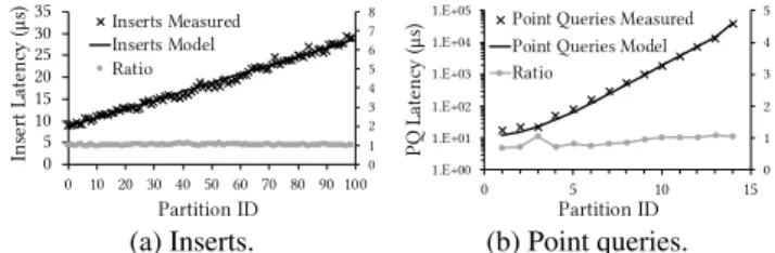
0 1 2 3 4 5 6 7 8 0 5 10 15 20 25 30 35 0 10 20 30 40 50 60 70 80 90 100 In se rt L ate nc y ( µs) Partition ID Inserts Measured Inserts Model Ratio 0 1 2 3 4 5 1.E+00 1.E+01 1.E+02 1.E+03 1.E+04 1.E+05 0 5 10 15 PQ L ate nc y ( µs) Partition ID Point Queries Measured Point Queries Model Ratio

(a) Inserts. (b) Point queries.

Figure 9: Cost model verification for (a) inserts and (b) point queries (10M chunk, exponentially increasing partition size).

cost udb(udbi) =cost pq(udbi) +udbi·(RR+2·RW) (14)

−udbi·(RR+RW)·trail parts(i)

cost utb(utbi) =utbi·(RR+RW)·trail parts(i) (15)

Overall Workload Cost.After deriving the cost for each operation per block, we can now express the total workload execution cost as a function of any given partition. This cost is given by Eq. 16, which adds the previously missing link of the workload cost in the optimization problem defined in Eq. 1. The Frequency Model now captures the data distribution and the access patterns of the opera-tions and the remaining free variable is the partitioning vector−→P.

cost−→P,F M=

N−1

∑

i=0

f ixed termi+bck termi·bck read(i)

+f wd termi·f wd read(i) +parts termi·trail parts(i)

(16)

where,∀i=0,1, . . . ,N−1:

f ixed termi=RR·(rsi+pqi+ini+dei+2·ud fi+2·udbi) +

SR·(rei+sci) +RW·(ini+dei+2·ud fi+2·udbi)

bck termi=SR·(rsi+pqi+dei+ud fi+udbi) (17)

f wd termi=SR·(rei+pqi+dei+ud fi+udbi)

parts termi= (RR+RW)·(ini+dei+ud fi−ut fi−udbi+utbi)

and F M={−RS→,SC−→,−RE→,−→PQ,IN−→,DE−→,−−−→U DF,U T F−−−→,−−→U DB,U T B−−→}. Note that the total cost in Eq. 16 is a function of quantities that ei-ther (a) depend on the Frequency Model only (f ixed termi,bck termi,

f wd termi,parts termi) or (b) depend on the partitioning strategy

and the Frequency Model (bck read(i),f wd read(i),trail parts(i)).

4.5

Cost Model Verification

The cost model captures the cost of the basic storage engine op-erations by accurately quantifying the cost of random and sequen-tial block memory accesses. As a result, the model only needs to tune very few parameters (the random and sequential memory block access costs for read and write operations). For every in-stance of Casper deployed, we first need to establish these values through micro-benchmarking. Subsequently, we can verify the ac-curacy of the overall cost model. It suffices to verify the estimated cost of insert and point read operations because they contain the two main cost functions of the model: (i) the number of trailing partitions for each partition (Eq. 8), and (ii) the size of each parti-tion, i.e., the sum off wd read(Eq. 4) andback read(Eq. 2).

Figure 9 shows that the proposed model accurately quantifies the costs of each operation using the fitted constants of the model. The random read latency and the random write latency in a memory block is 100ns, while the sequential read is amortized, leading to 14×lower cost per block. We further observe that the partition in-dex has a cumulative cost of 8.5µsper operation, which is shared across all operations and does not influence the partitioning pro-cess. Figure 9a shows the measured and the model-based insert cost when using chunks of 10M elements, each with 100 partitions. The experiment corroborates a strong linear relation of the cost to the

number of trailing partitions. Figure 9b shows the measured and the model-based point query cost. In this experiment, the chunk has 15 partitions with exponentially increasing size, ranging from 29elements for the first partition to 222elements for the last parti-tion. Here the experiment supports a strong linear relation between the cost of a point query and the partition size. Note that in both figures the grey points indicate the ratio between the measured and the model-based cost which is always very close to 1.0 (y-axis on the right hand-side).

4.6

Considering Ghost Values

Ghost Values Benefit Performance.Ghost values enable a trade-off between memory utilization and data movement. In particular, delete operations simply create a hole in the partition they target. Insert operations do not need to create space by rippling if there are available ghost values. Finally, update operations can create a new empty slot in the partition they update from and simply use available slots to store the new values.

Distributing Ghost Values to Partitions. Given−→P,

F M

way that minimizes the overall cost. The operations that can bene-fit from having ghost values in the partitions they target areinserts andupdates. For every partition that an operation inserts into, a ghost value can help to entirely avoid the ripple insert. Similarly, for every update operation (either with forward or backward rip-ple), the partitions that have incoming updates will avoid a ripple insert (in the worst case) by using the available ghost values. To cover this worst case, in the remainder of the ghost value analysis, we consider that everyinsertandupdate tooperation requires a rip-ple insert. The distribution of ghost values for blocki,GValloc(i)

is given by Eq. 18, which uses the data movement per block as a result of inserts and updates(dm part(i)), as well as the total data movement (dm tot), to distribute ghost values proportionally to the performance benefit they offer.

GValloc(i) =

dm part(i)

dm tot ·GVtot (18)

5.

OPTIMAL COLUMN LAYOUT

Minimizing Total Workload Cost.Using the column layout cost model, we formulate the following optimization problem:

minimize ∑Ni=−01 f ixed termi +bck termi·∑ij−=10∏ki−=1j(1−pk) +f wd termi·∑Nj=−0i−1∏ N−j−1 k=i (1−pk) +parts termi·∑Nj=−i1pj subject to pN−1=1 pi∈ {0,1}, i=∈ {0,1, . . . ,N−2} (19)

The constraint pN−1=1 guarantees that the dataset forms at least one partition (zero partitions has no real meaning), andpi∈

{0,1}guarantees that eachpiis a binary variable.

The binary optimization problem formulated above, however, contains products between groups of variables, and cannot be solved by linear optimization solvers. Products between variables can be replaced by new variables and additional constraints [22]. The final binary linear optimization problem formulation is shown in Eq. 20. Note the new constraints on the two-dimensional variables yi,j, which guarantee that eachyi,j corresponds to the product it

replaced.

Performance Constraints.The minimization in Eq. 20 is also aug-mented with performance SLAs. In particular, an application may

online model training

Mosek BIP solver

Casper

Core Storage Engine

Storage Engine API re ad/wr ite ope rations offline workload model training partitioning workload model Partitioner applying physical layout

B

C

A

’

A

Figure 10: System architecture. (A) Casper uses offline work-load information, (B) solves the BIP and (C) applies the par-titioning. (A0) During execution monitoring, if the access pat-terns change, a re-partitioning cycle is triggered.

require read queries to respect areadSLA, or updates to respect an

updateSLA. Such constraints are expressed as a function of

− →

P.

minimize ∑Ni=−01

f ixed termi+bck termi·∑ij−=10yj,i−1

+f wd termi·∑Nj=−0i−1yi,N−j−1 +parts termi·∑Nj=−i1pj subject to pN−1=1 pi∈ {0,1}, i=∈ {0,1, . . . ,N−2} yi,i=1−pi, i=∈ {0,1, . . . ,N−1} yi,j≤1−pj, i,j=∈ {0,1, . . . ,N−1},i<j yi,j≥1−∑kj=ipk yi,j∈ {0,1} (20)

Update Latency Constraint. An update/insert SLA dictates that all update/insert operations are faster than a maximum allowed la-tencyupdateSLA. The most expensive operation has to ripple through

all partitions, so this constraint can be expressed as follows:

(RR+RW)·(1+ N−1

∑

∑

Read Latency Constraint. A SLA for read queries dictates the maximum read cost for a point query, which in turn, is quantified by the size of the maximum allowed partition size (MPS), as follows:

RR+SR·MPS=readSLA⇒MPS=

readSLA−RR

SR

In order to ensure that the largest partition is at mostMPSblocks wide, we need to make sure that for everyMPSconsecutivepi’s at

least one of them is equal to 1. In other words∀j=0, . . . ,N−MPS:

∑MPS_i=0−1pj+i≥1.

Overall, the performance constraints augment the binary linear optimization formulation with the following bounds:

bounds ∑Ni=−01pi≤updateRR+RWSLA−1

∀j={0,1, . . . ,N−MPS}: ∑iMPS=0−1pj+i≥1 whereMPS=readSLA−RR

SR −1

(21)

Adding the bounds of Eq. 21 to the optimization problem in Eq. 20 completes the formalization of partitioning as a binary linear optimization problem, for which we use the Mosek solver [8].

6.

Casper STORAGE ENGINE

We implement the Casper storage engine in C++. Casper fully supports all five access patterns described in Section 3, effectively being a drop-in replacement for any relational scan operator with support for updates. Casper supports all the common access pat-terns, hence, it provides general support for accessing data for re-lational operators. The size of the code added to implement the Casper column layout decision method described in Sections 4 and 5 is in the order of 4K lines of code. Figure 10 shows the overall ar-chitecture of Casper. The key components are (i) the Frequency Model that maintains an accurate estimation of the access patterns

over the physical storage, (ii) the optimization component that em-ploys the state-of-the-art solver Mosek [8], (iii) the partitioner that implements the physical layout decisions, and (iv) the core storage engine that implements the update and access operations over the partitioned data. Casper naturally supports multi-threaded execu-tion since the column layouts create regions of the data that can be processed in parallel without any interference. Some of the op-erations require to update the contents of other partitions (when a ripple is necessary), hence, correct execution needs a way to pro-tect the atomicity of each operation through snapshot isolation or locking. Ghost values allow Casper to reduce contention by allow-ing an update, delete or insert, to affect in the best case, only one partition and avoid rippling.

6.1

Transaction Support

Hybrid workloads consist of long-running analytical queries and short-lived transactions. The systems that support hybrid work-loads must ensure that the long running queries are executed with-out being affected by the transactions, neither with respect to per-formance, nor the correctness of the values read. Casper supports general transactions through snapshot isolation [20], which isolates a snapshot of the database observed at the beginning of each trans-action, and works only on that.

Snapshot Isolation through Multi-version Concurrency Con-trol.Recent HTAP systems and storage engines employ variations of multi-version concurrency control (MVCC) [11, 58, 74, 76] that allows for snapshot isolation [20]. Casper takes a similar approach: each transaction is allowed to work on the data by assigning times-tamps to every row when inserted or updated, initially maintained in a local per-transaction buffer. For the frequent cases, the short-lived transactions will be operating over disjoint sets of rows hence there will be no conflicts. In the rare case that multiple transactions are trying to access the same object, the first one to commit wins and the other transactions abort and roll back.

Reducing the Ripple Contention. In order to reduce the con-tention of moving ghost values to the partition we are inserting into, (i) Casper moves a block of ghost values every time one is neces-sary, which can be used by neighboring partitions in the future, and (ii) we decouple the ghost value rippling from the transaction since it does not affect correctness. Hence, even if a transaction is rolled back, the already completed fetching of ghost values will persist and will benefit future inserts or updates.

6.2

Compression

Casper natively supports thedictionaryandframe-of-reference (or delta) compression schemes, the most commonly employed in

modern column-store data systems [1, 2, 85]. First, dictionary

compression is supported by Casper as-is. The performance con-stants of the model are changed to reflect the compressed data size, and Casper’s behavior remains qualitatively the same. Second,

whendeltaencoding is used, a synergy between the partitioning

and the compression effort is created. In fact, Casper tends to finely partition areas that attract more queries, thus, enabling better delta compression since the value range of small partitions is also small. This has a multiplicative impact on the savings in memory band-width per item. The more we read a partition the more compressed it is, leading to less overall data movement. Casper compresses our micro-benchmark data by 2.5×and TPC-H data by 4.5×.

Another compression approach used in columnar systems is run-length encoding (RLE) [2]. RLE requires the data to be sorted in order to calculate the run lengths, and it always requires a more expensive “decoding” step when updating (similar to bit-wise RLE for bitmap indexes [16]). RLE often has better compression rate

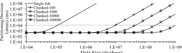
1.E+01 1.E+02 1.E+03 1.E+04 1.E+05 1.E+06 1.E+07 1.E+08

1.E+04 1.E+05 1.E+06 1.E+07 1.E+08 1.E+09

Pa rt it ioni ng D ec is ion L at enc y (m s)

Data Size (#values) Single Job

Chunked-100 Chunked-1000 Chunked-10000 Chunked-100000

Figure 11: Casper partitioning scales with data size.

than dictionary or delta compression, however, it has higher con-struction cost (it needs sorting), higher execution cost (decoding) and higher update cost (decode/re-encode). Hence, typically dictio-nary and delta compression schemes are preferred over RLE [85].

6.3

Scalability with Problem Size

Casper formulates and solves a binary integer problem withN bi-nary variables, having an exponential (2N) solution space. Modern optimization techniques allow to search this space in polynomial time. In particular, we use the optimization problem solver Mosek, which relaxes non-convex problems using semidefinite optimiza-tion [8]. This allows the Casper column layout decision process to have cubic complexity. For a dataset withMvalues, andBvalues per block, Casper needsO((M/B)3)time. In order to maintain the column layout decision cost low, we can either increase the block size or divide the problem into smaller sub-problems by creatingC chunks. The former produces solutions with lower quality (coarser partitioning granularity), hence, using column chunks is preferred. The histograms are created per chunk, and, similarly, design deci-sions are made for each chunk without any need for communication with other chunks. This allows us to arbitrarily reduce the partition-ing complexity. For a level of parallelism equal toCPU, we execute

CPUsub-problems at the same time and exploit their

embarrass-ingly parallel nature for an overall costO((C/CPU)·(M/(B·C))3). In practice, we find the optimal layout of a 109_{-element relation} using 64 cores and a block size of 4096 bytes, in about 10 seconds (Fig. 11), while the estimated time without chunking and paral-lelism is 1015seconds.

Variable Histogram Granularity. Casper can vary the granular-ity of the histograms to match a multiple of the page size either by aggregating histogram values, or by using data and access distribu-tions to calculate coarser granularity histograms (following §4.3).

Locating Partitions. Casper stores partition-wise metadata to be able to find and discard partitions for each query. For every par-tition, the minimum and the maximum value of the domain they cover is stored, along with positional information within the chunk. The metadata enable efficient searching with a k-ary search tree. If the chunk size is small or the average partition size is large, the number of partitions is small enough to fit in the higher lev-els of cache memory. In that case, the metadata can be treated as Zonemaps [35, 55] and they can be very efficiently scanned.

6.4

Casper as a Generic Storage Engine

Casper implements a repertoire of standard storage engine API calls including (i) scanning an entire column (or groups of columns), (ii) search for a specific value, (iii) search for a specific range of values, (iv) insert a new entry, and (v) update or delete an exist-ing entry. This generic API is supported by systems that target either analytical or transactional workloads and is compatible with state-of-the-art storage engines [57]. As a result, Casper can be easily integrated into existing systems. Note thatmixed workloads refer to interleaving long read queries with short updates/inserts. Similarly to both transactional-optimized and analytical-optimized storage engines, Casper supports all operations. Using workload

1.75 2.14 1.16 0.95 2.28 2.32 0.0 0.5 1.0 1.5 2.0 2.5

hybrid, skewed hybrid, range, skewed read-only, skewed read-only, uniform update-only, skewed update-only, uniform

N orm . T hr ou ghp

ut Casper Equi-GV Equi

State-of-art Sorted No Order

Figure 12: Casper matches or significantly outperforms other column layouts approaches for a variety of workloads (experiments with 16 threads, chunks of 1M values, block size 16KB, and ghost values 0.1%).

knowledge, Casper offers physical layouts for hybrid workloads that outperform state-of-the-art physical designs.

Multi-Column Range Queries. Casper natively supports multi-column range queries. Similar to state-of-the-art storage engines, Casper evaluates the first (typically the most selective) filter and retrieves the qualifying positions to evaluate the subsequent filters (further accelerated using Zonemaps [55]). We refer to Figure 1 for an experiment with multi-column range queries (TPC-H Q6 [81]) that shows Casper outperforming the state of the art by 2.5×.

7.

EXPERIMENTAL EVALUATION

Experimental Setup. We deploy Casper in a memory-optimized server from Amazon EC2 (instance type m4.16xlarge) with a 64-bit Ubuntu 16.04.3 on Linux 4.4.0. The machine has 256GB of main memory and two sockets each having an Intel Xeon E5-2686 v4 processor running at 2.3GHz with 45MB of L3 cache. Each pro-cessor supports 32 hardware threads (a total of 64 for the server).

Experimental Methodology. For fair comparison, Casper inte-grates all tested column layout strategies. In particular, Casper has six distinct operation modes: (i) plain column-store with no data organization (No Order), (ii) column-store with sorted data in the leading column (Sorted), (iii) state-of-the-art update-aware column-store with sorted columns and a delta store for incoming updates (State-of-art), (iv) column-store with equi-width partitioned data (Equi), (v) column-store with equi-width partitioned data and ghost values (Equi-GV), and (vi)Casperthat puts everything to-gether. For fairness and in order to have low experimental design complexity, we allow Casper to have as many partitions as the equi-width partitioning schemes, but it has the freedom to allocate their sizes according to the optimization problem.

Column Chunks.The storage engine uses a column-chunk based layout. Each column is not a single contiguous column; instead, it is a collection of column chunks, each one stored and managed sep-arately. This technique is employed by numerous modern systems giving flexibility for updates [30], and serves as the main state-of-the-art competitor in our experimentation. We use column chunks that hold 1M values each. Unless otherwise noted, we use 16 threads. Each experiment comprises of 10000 operations. We re-peat each experiment multiple times, and we report measurements with low standard deviation.

7.1

HAP Benchmark

We first describe the evaluation benchmark. Since there is cur-rently a scarcity of benchmarks for hybrid workloads we develop our own benchmark that we call Hybrid Access Patterns (HAP) benchmark. HAP is based on the ADAPT benchmark [11], and is composed of queries that are common in enterprise workloads [68], as well as transactional (small) general update queries that are typ-ically tested in hybrid storage engines [25, 31].

The HAP benchmark has two tables, a narrow table with 16 columns and a wide one with 160 columns. Each table contains tu-ples with a 8-byte integer primary keya0and a payload ofp4-byte

columns(a1,a2, . . . ,ap). In all of our experiments, we load 100M

tuples in the database in order to report a steady-state performance. The benchmark consists of six queries:(Q1)apoint querythat requests the contents of a row,(Q2)anaggregate range querythat counts the rows in a range, (Q3)anarithmetic range querythat sums a subset of attributes of the selected rows, (Q4) aninsert query that adds a new tuple in the relation, (Q5)adeletequery that deletes a specific tuple, and(Q6)anupdatequery that fixes an error in a data entry by correcting its primary key value. The SQL code for each of the queries is available below:

Q1:SELECTa1,a2, . . . ,akFROMRWHEREa0=v Q2:SELECTcount(∗)FROMRWHEREa0∈[vs,ve)

Q3:SELECTa1+a2+· · ·+akFROMRWHEREa0∈[vs,ve)

Q4:INSERT INTORVALUES(a0,a1,a2, . . . ,ap)

Q5:DELETE FROMRWHEREa0=v Q6:UPDATERSETa0=vnewWHEREa0=v

With different values ofk,v,vs, andve, we test various different

aspects of the workloads including projectivity, selectivity, overlap between queries, and hot and cold regions of the domain. Unless otherwise noted, we experiment with datasets of 100M tuples and 16 columns, with uniformly distributed integer values.

Logical and Physical Benchmarking. We develop a specialized benchmark for storage engines for hybrid workloads, which we view as a “physical” benchmark for the supported access paths. Similar to recent research on new storage engines, we stress-test the access path and the update performance [11, 25, 28, 31].

To stress different aspects of Casper, we test various combina-tions of queriesQ1throughQ6. In particular, we synthesize three different types of workloads: (i)hybrid, (ii)read-only, and (iii)

update-only. We have two versions of the hybrid workload, one

withQ1 andQ4 that has equality searches and one withQ3and Q4that has range searches. For the read-only and the update-only workloads we have two versions: one with uniform accesses and one with skewed accesses. Every workload has a small fraction (1%) of updates (Q6) uniformly distributed across the whole do-main to mimic updates and corrections frequently taking place in mixed analytical and transactional processing.

7.2

Casper Improves Overall Throughput

Figure 12 shows that Casper matches or significantly outper-forms most of the different approaches frequently used for han-dling hybrid workloads. The figure compares the throughput of all tested approaches normalized against the column-store state-of-the-art design that employs a delta store. The first two workloads are hybrid with skewed accessed to more recent data. The main dif-ference between the two is that the first has equality queries (Q1) and the second has range queries (Q3). Casper leads to a 1.75×to

2.14×performance improvement over the state of the art. With

respect to the different configurations we tried, we observe that equi-width partitioning is slower than the state of the art (equal-ity queries have to read whole partitions even when not needed), while it actually leads to a small performance improvement for

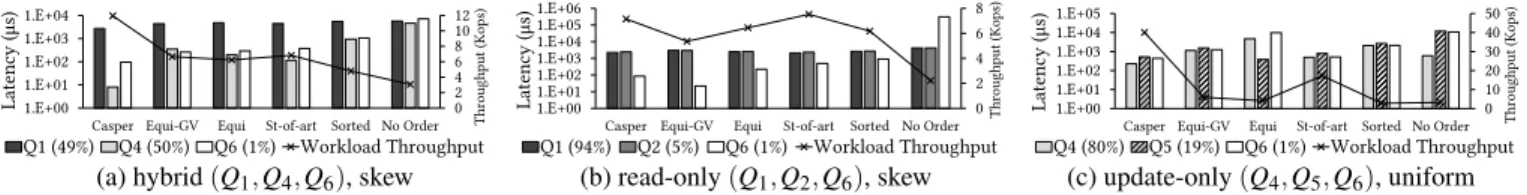
0 2 4 6 8 10 12 1.E+00 1.E+01 1.E+02 1.E+03 1.E+04

Casper Equi-GV Equi St-of-art Sorted No Order Thr

oug hp ut (Ko ps) Late ncy (μs) Q1 (49%) Q4 (50%) Q6 (1%) Workload Throughput 0 2 4 6 8 1.E+00 1.E+01 1.E+02 1.E+03 1.E+04 1.E+05 1.E+06

Casper Equi-GV Equi St-of-art Sorted No Order T

hro ug hpu t (K ops) Laten cy ( μs) Q1 (94%) Q2 (5%) Q6 (1%) Workload Throughput 0 10 20 30 40 50 1.E+00 1.E+01 1.E+02 1.E+03 1.E+04 1.E+05

Casper Equi-GV Equi St-of-art Sorted No Order Thr

oug hpu t ( Ko ps) Laten cy ( μs) Q4 (80%) Q5 (19%) Q6 (1%) Workload Throughput

(a) hybrid(Q1,Q4,Q6), skew (b) read-only(Q1,Q2,Q6), skew (c) update-only(Q4,Q5,Q6), uniform

Figure 13: Casper offers significant performance benefits. In (a) for a hybrid workload with skewed point queries and inserts, Casper outperforms all approaches by balancing the read and update performance. In (b) for a read-heavy workload with range queries, point queries, and a few inserts, Casper matches the state-of-the-art delta-store design. Finally, in (c) for an update-only workload, Casper significantly outperforms by 2×or more all other approaches .

0 10 20 30 40 50

UDI1 UDI2 YCSB-A2

Ins er t Lat. (μs ) _{0.01% 0.1% 1% 10%} update-only,

skewed update-only, uniform hybrid, skewed Figure 14: Using ghost values (4 thr., 1M chunks, 16KB blocks).

0 1 2 3 1.E+00 1.E+01 1.E+02 1.E+03 None 12.5 10 7.5 6.25 3.75 2.5 2 1.5 Th rou ghpu t (K ops) La tency (μs ) Insert SLA (μs) Q1 (89%) Q4 (10%) Q6 (1%) Throughput Figure 15: Casper meets performance SLA executing a hybrid workload(Q1,Q4,Q6)(1M chunk size, 16KB block size).

range searches. As Casper targets mixed workloads, it cannot al-ways offer the best performance for read-only workloads (Q1and Q2). In particular, the state of the art has 5% higher throughput for skewed read-only queries. On the other hand, for uniform accesses, Casper leads to 1.44×higher throughput. For these cases, however, even simply equi-width partitioning and maintaining data sorted on the search attribute delivers competitive performance. Finally, for the update-intensive workloads (Q4 andQ5), Casper offers 2.28-2.32×higher throughput by exploiting ghost values and avoiding frequent data reorganization (which the state of the art does).

7.3

Casper’s Impact on Update Performance

Casper Offers Better Read/Write Balance.Next, we drill-down to understand where the benefits of Casper come from, by measur-ing the latency of each operation for each workload in Figure 13. For the hybrid workload with equality queries and skewed accesses (Fig. 13a), Casper offers three orders of magnitude faster inserts (Q4) than the other column layouts without hurting the latency of

Q1. For a read-only workload with both equality searches and

range searches (Fig. 13b), even a small number of updates (<1% of the workload) disrupts the performance of all other column lay-outs except Casper. The reason is that Casper executes read queries without having as many partitions as the equi-width partitioned ap-proaches, nor having the cost to maintain and continuously inte-grate a delta storage. For the update-only workload, the difference is more pronounced (Fig. 13c); Casper limits the number of parti-tions and distributes more effectively the ghost values.

Casper Leverages Ghost Values.We now demonstrate that Casper can leverage ghost values to optimize inserts. Figure 14 shows that insert latency scales as we increase the number of ghost values from 0.01% of the dataset to 10%, for update-intensive and hybrid

work-PQ Insert histogram 0.0 0.5 1.0 1.5 0% 5% 10% 15% 20% 25% 30% 35% 40% 45% 50% No rm . L at ne nc y rotational shift -25% -15% 0% +15% +25% mass shift

(a) Workload histograms (b) Normalized latency

over normalized domain. with workload uncertainty.

Figure 16: Testing Casper’s robustness.

loads. We observe that in all cases Casper takes advantage of the additional ghost values to further reduce the insert latency; using as low as 1% ghost values, Casper reduces insert latency by 2×.

7.4

Meeting Performance Constraints

Our next experiment showcases how Casper matches a given performance requirement without sacrificing overall system perfor-mance using a hybrid workload with equality searches (Q1), inserts (Q4), and a tiny fraction of updates (Q6). Figure 15 shows the la-tency of each query, as well as the system throughput for different insert SLAs on the x-axis. When no SLA is set, Casper achieves the highest throughput. As we decrease the maximum allowed in-sert latency, the inin-sert cost decreases proportionally (we report both the average and the 99.9% percentile with the error bars), with neg-ligible impact on the overall system throughput. Interestingly, for lower insert SLA the update cost increases. The lower insert la-tency is achieved by having fewer partitions. This leads to more ex-pensive point queries to locate the deleted value when executing the delete part of the update. Casper balances the overall throughput and respects the insert SLA with a small performance hit (<3%).

7.5

Robustness to Workload Uncertainty

Our final experiment tests the robustness of the physical layout proposed and shows that Casper is robust up to a level of workload uncertainty, after which, there is a performance cliff. Figure 16a shows a summarization of the histograms used as input to the Fre-quency Model for point queries and inserts. Both operations occur with frequency 50%, however, point queries mostly target the latter part of the domain, and inserts the first part of the domain. Next, we consider two types of uncertainty in Figure 16b: (i) mass shift from point queries to inserts (shown as different lines), and (ii) rota-tional shift with respect to the targeted part of the domain (x-axis). Figure 16b shows that Casper offers a robust physical layout which abso