Learning Active Contour Models for Medical Image Segmentation
Xu Chen
1, Bryan M. Williams
1, Srinivasa R. Vallabhaneni
1,2, Gabriela Czanner
1,3, Rachel Williams
1,
and Yalin Zheng
11
Department of Eye and Vision Science, Institute of Ageing and Chronic Disease, University of
Liverpool, L7 8TX, UK
2
Liverpool Vascular & Endovascular Service, Royal Liverpool University Hospital, L7 8XP, UK
3Department of Applied Mathematics, Liverpool John Moores University, L3 3AF, UK
{xuchen, bryan, fempop, g.czanner, rlw, yzheng}@liverpool.ac.uk
Abstract
Image segmentation is an important step in medical im-age processing and has been widely studied and developed for refinement of clinical analysis and applications. New models based on deep learning have improved results but are restricted to pixel-wise tting of the segmentation map. Our aim was to tackle this limitation by developing a new model based on deep learning which takes into account the area inside as well as outside the region of interest as well as the size of boundaries during learning. Specically, we propose a new loss function which incorporates area and size information and integrates this into a dense deep learn-ing model. We evaluated our approach on a dataset of more than 2,000 cardiac MRI scans. Our results show that the proposed loss function outperforms other mainstream loss function Cross-entropy on two common segmentation net-works. Our loss function is robust while using different hy-perparameterλ.
1. Introduction
Image segmentation is a fundamental and challenging problem in computer vision, with the aim of partitioning an image in a meaningful way so that objects can be localized, distinguished and/or measured. In medical imag-ing, this is vital for further clinical analysis, diagnostics, treatment planning and measuring disease progression. High precision is typically required in bio-medical image segmentation [6, 24]. Recently, segmentation techniques based on deep convolutional neural networks (CNNs) have been developed for various medical imaging modalities, such as MRI, CT and X-ray, showing promising results and overcoming the limitations of conventional segmentation
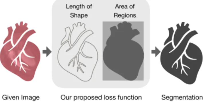
Figure 1: Our proposed loss function
methods [17]. During the training process of a CNN model, its parameters are optimized through gradient descent approaches based on the errors measured by a loss function, which compares the prediction and ground truth images. Loss functions are critical for model optimization. In terms of classification problems, the L2 norm is also known as mean squared error (MSE) and cross-entropy (CE) are commonly used as loss functions [8, 33]. CE and the Dice coefficient (DC) have typically been used for segmentation problems [24, 12].
Despite the recent progress of using CNNs for bio-medical image segmentation, the commonly used loss functions generally evaluate pixel-wise similarity. For instance, CE and DC focus on extracted features from specific regions [28]. While this can result in good clas-sification and segmentation performance, low resultant loss function values may not necessarily correspond to a meaningful segmentation. For example, a noisy result can add many contours in the background representing incorrect segmentation, and object boundaries can be fuzzy
due to the difficulty of classifying pixels near the boundary. We propose to address these issues by (i) building the length of the boundary segmentation contour into the loss function so that this is constrained and (ii) considering the fitting inside and outside of the estimated boundaries in order to preserve shape.
According to the WHO, cardiovascular disease (CVD) is the world’s number one killer, taking 17.9 million lives per year. The segmentation of Cardiac Magnetic Reso-nance (CMR) images is important for the assisted diag-nosis of CVD. However, there are a limited number of fully-automatic segmentation methods, which is essential for CVD diagnosis. Our segmentation work is part of the effort to address this global challenge by developing new solutions for the accurate and reliable analysis of CMR im-ages for improved decision making.
1.1. Contributions
To the best of our knowledge, this is the first work which integrates length and region constraints into the loss func-tion of CNN-based segmentafunc-tion, as shown in Figure 1. The contributions of this work are:
• We develop a new loss function combining contour length and region information.
• Based on this, we develop a CNN model based on con-ventional Dense U-Net.
• We evaluate our model in a supervised bio-medical segmentation setting for CVD diagnosis.
2. Related Work
In this section, conventional and CNN-based segmenta-tion methods and related to this work briefly reviewed in the following context.
2.1. Conventional Segmentation Methods
In the past few decades, various models have been pro-posed ranging from thresholding, edge detection, cluster-ing, region-growing to more complex active contour mod-els. Early models such as thresholding and region growing approaches are able to implement but the performance is limited due to its nature of using image intensity or texture information only [7]. Active contour models (ACMs) have shown more performance as represented by the active con-tour without edge (ACWE) model [4] and also Mumford-Shah’ work [21]. In Chan and Vese’s work, level set func-tions are introduced to formulate the segmentation model treated as an energy minimization problem solved through solving partial differential equations (PDEs). Later on, this model has been extended to multiphase problems and tex-ture problems [31, 29]. Efficient solvers such as dual pro-jection and graph cut methods have been introduced to
im-prove the computational efficiency [20]. The common chal-lenges for these models are time-consuming. On the other hand, supervised segmentation models based on feature ex-traction and neural networks or support vector machines also showed reasonable results. However, these models are based on hand-craft features for the segmentation thus de-pendent on the skills and experience of the researchers so it’s limited applicability and result quality.
2.2. CNN-based Methods for Segmentation
As a class of deep neural networks, CNNs show remark-able performance in many computer vision tasks, such as classification, segmentation and registration. One of the particular strength of CNN based models is that they work in an end-to-end fashion, which can extract hierarchical and multi-resolution features during the learning process. CNN architectures like Alex-Net [14], VGG-Net [25], Google-Net [26] and Dense-Google-Net [9] have been developed and intro-duced into various image recognition tasks. Broadly speak-ing, CNN based segmentation models can be classified into pixel-based or images-based approaches. The pixel-based approaches will classify each pixel into different objects as a classification problem. A patch is often produced for each pixel (or super-pixel) and the patch is used as input to CNN models for classification with the label of the pixel used as the target to train the model [5]. The image-based ap-proaches, such as U-Net [24], will make an image as input and output will be the segmentation of the input image (the size will be the same). U-Net like models have become pop-ular because of its good performance and simplicity when compared to pixel-wise approaches [28, 15, 12](Please sort out these references). However, due to the lack of consider-ation on outside the target so that small segmented objects occur around the boundaries. In order to tackle this prob-lem, a network based on Dense-Net called one hundred lay-ers Tiramisu was proposed byJégou et.al[12] making each layer to connect with others in a feed-forward fashion for encouraging extracted features to reuse and for strengthen-ing feature propagation so that Dense-Net can reduce the influence from outside features of targets. Dense-Net over-comes this limitation of U-Net in various medical image applications [15][12]. However, some researchers prove that developing different loss functions is also able to im-prove the performance of U-Net during the training process [18, 27, 1]. Arif et.al[1] address the gap by introducing a shape-aware term in the segmentation loss function. Their approach significantly improved the performance of cervi-cal X-ray images by 12%. Inspired by the recent progress in loss function, we present a novel loss function borrowed from the conventional model to further improve the segmen-tation performance.
2.3. Loss functions
To train a CNN model, the loss function (or cost func-tion) plays a significant role. Loss function is a function to measure the error of prediction or segmentation which can be back propagated to previous layers in order to up-date/optimize the weights. Here, we briefly review the commonly used loss functions. In the following equations, ground truth image (or expert annotation) and the prediction (or segmentation) is denoted asT,P ∈ [0,1]m×n
respec-tively;nindexes each pixel value in image spatial spaceN; the label of each class is written aslinCclasses.
Cross-Entropy (CE) Loss:CE is a widely used pixel-wise measure [24] to evaluate the performance of classification or segmentation model. For two-class problems, CE loss function can be expressed as Binary-CE (BCE) loss func-tion as follows: LossBCE(T, P) = −N1 N X n=1 Tn·log(Pn) + (1−Tn)·log(1−Pn)
CE loss functions treat the output from softmax layer as a pixel classification problem to evaluate each pixel. Ron-neberger et al. [24] pointed out that in order to improve the performance in cells’ border segmentation from bio-medical images, CE loss function with weighting scheme can be as one of the solutions to help U-Net model segments cells border as accurately as possible. Moreover, there are numerous studies on CE-based loss functions but merely a few functions consider the geometric detail of objects [16]. Dice Coefficient (DC) Loss: DC is traditionally used as a metric for the evaluation of the segmentation performance and now also demonstrated a good performance as a loss function [19]. DC measure the degree of overlapping be-tween the reference and segmentation. This element-wise measure ranges from 0 to 1 where a DC of 1 denotes per-fect and complete overlap. DC can be defined as:
DC(T, P) = 2· PN n=1(Tn×Pn) PN n=1(Tn+Pn) (1)
DC loss is defined in Eq.(2) as it tends to the best segmen-tation.
LossDC(T, P) = 1−DC(T, P) (2)
Even though CE and DC loss functions have achieved a suc-cess in image segmentation, there are two main limitations: they are pixel-wised loss functions to measure the similarity betweenT andP, but the geometrical information are not taken into consideration.
2.4. Active Contour Models
In this section, we provide some background knowl-edge of the ACMs firstly proposed by Kass et al. [13]. ACM models treat segmentation as an energy minimiza-tion problem where the energy of an active spline/contour is minimized by PDEs-based methods toward the objects’ boundaries. In classic ACMs, detecting objects’ boundaries is by image gradients. However, this has one main lim-itation that it will be stuck at a local minimum. There-fore, it cannot get satisfactory segmentation results. In the past two decades, a number of ACMs have been pro-posed, such as active contour without edge (ACWE) model and fast global minimization-based active contour model (FGM-ACM) proposed byBresson et al.[3].
The ACWE model can be formulated as the following en-ergy minimization problem:
min Ωc,c1,c2{ EACW E1 (Ωc, c1, c2, λ) = Z Length(C) 0 ds +λ Z Ω (c1−f(x))2dx +λ Z Ω/Ωc (c2−f(x))2dx}, (3) wheredsis the Euclidean element of length, the first term of Eq.(3) is the length of the curveC, andf is the image to be segmented,Ωcis a closed subset of the imagef domain
Ω. The mean value off outside and inside are denoted as c1 andc2, respectively. λ is an arbitrary fixed parameter (λ >0) to controls the balance between regularization pro-cess andc1,c2. The energyEACW E
1 (3) can improve be-cause it naturally adds more constraints including the con-tour length than DC and CE loss function. In order to solve the segmentation formulation, Heaviside function of level set method and PDEs were introduced to decrease the en-ergyEACW E
1 .E1ACW Ecan be rewritten as follows: EACW E2 (Ωc, c1, c2, λ) = Z Ω ∇Hǫ(φ) dx +λ Z Ω Hǫ(φ)(c1−f(x))2dx +λ Z Ω/Ωc Hǫ(−φ)(c2−f(x))2dx ) (4) where Hǫ is a smooth approximation of the Heaviside
function. And the gradient descent method minimizing of EACW E 2 (4) is defined as: ∂tφ=Hǫ′(φ) ( div ∇φ |∇φ| −λr1(x, c1, c2) ) (5)
wherer1(x, c1, c2) = (c1−f(x))2−(c2−f(x))2shown in Eq.(5). However, PDEs-based solutions including ACWE need to be solved on each individual image, which is time-consuming. While they can give very good results, this makes ACWE less suitable for application in clinical set-tings where fast results, often as short as a few seconds, are needed. In order to achieve global minimization fast and stable, aEACW Ebased on total variation energyT V was
proposed [3] which is defined as in Eq.(6): E4ACW E(u, c1, c2, λ) =T Vg(u) +λ
Z Ω
r1(x, c1, c2)udx (6) whereuis a characteristic function 1Ω
c. T Vg(u) is total
variation energy. Eq.(6) can also be written as:
E4ACW E(u, c1, c2, λ) = Z Length(C) 0 g|∇u|ds | {z } Length +λ Z Ω ((c1−f(x))2−(c2−f(x))2)udx | {z } Region (7)
where,uis a characteristic function valued between 0 and 1. EACW E
4 (7) provides a global minimum for ACWE model. Moreover, due to the limitation of the previous version of ACWE model based on Heaviside function and PDEs-based solutions, it provides a fast and non-stationary so-lution while uis restricted from0 and1. And also, this minimization problem of ACME to carry out segmentation task is able to apply into the deep learning field as it is con-strained and some parameters can be fixed due to super-vised learning and some parameters can be treated as train-able parameters to evaluate this minimization equation in an end-to-end learning fashion. In the §3 we will present more details of it.
3. Our Method
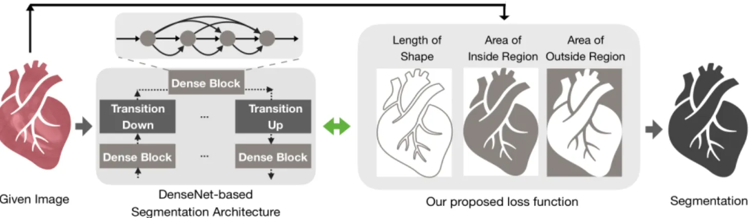
We propose a loss function inspired by the general idea of active contour model building in region and length terms for bio-medical image segmentation by U-Net-like based deep learning architectures. The work-flow is displayed in Figure 2. Our loss function denoted as AC, is in §3.1. Our main CNN Architecture in §3.2 is introduced.
3.1. AC Loss Function
The idea of proposed AC loss is behind the minimization problem of ACWE model (6) to efficiently find an active contour which is a global minimization of active contour energy for automated image segmentation. In the follow-ing equations, ground truth (reference segmentation) and
the predicted value is denoted asv,u∈ [0,1]m×n
respec-tively. A 2-dimensional example of our AC loss function is defined as follows:
LossAC=Length+λ·Region, (8)
in which, Length= Z C|∇ u|ds (9) Region= Z Ω ((c1−v)2−(c2−v)2)udx (10) Therefore,LengthandAreaof Eq.(9) and Eq.(10) can be written into pixel-wised way respectively as follows:
Length= i=1,j=1 X Ω q (∇uxi,j) 2+ (∇u yi,j) 2+ǫ (11)
where,xandyfromuxi,janduyi,jare horizontal and
verti-cal directions respectively.ǫ(ǫ >0)is a parameter to avoid square root is zero in practice.
Region = i=1,j=1 X Ω ui,j(c1−vi,j)2 + i=1,j=1 X Ω (1−ui,j)(c2−vi,j)2 (12)
where, in the ACWE model 3, c1 andc2 are variable and defined as follows: c1= R v·udx/R udx c2=R v·(1−u)dx/R(1−u)dx (13)
due to supervised-learning framework, c1 andc2 are rep-resented as the energy of inside (foreground) and outside (background) and can be simply defined as constants in ad-vance asc1 =1andc2 = 0. uandv are represented as
prediction and a given image respectively. In practice, we setǫ = 10−6as a small positive number to avoid the √0
issue in Tensorflow initialization. Therefore, we proposed a new loss function building on the length of the boundary segmentation contour and considering the region fitting for not only has the same nature of non-convex from Eq.(7) but also our new loss function is fit for shape preservation.
3.2. CNN Architecture
In this subsection, we detail and use U-Net [24] and dense U-Net [24] architectures as our base segmentation frameworks to evaluate our proposed loss function perfor-mance. Recently, U-Net is proposed and widely used which is an end-to-end and encoder-decoder neural network for se-mantic segmentation with high precise results. As one of the
Figure 2: Overview of our proposed method which takes the object’s area and length of the boundaries into account during training.
essential building blocks is skipped connections which are designed for forwarding feature maps from down-sampling path to the up-sampling path in order to localize high res-olution features to generate a segmentation output. In the down-sampling path, each layer consists of two 3×3 convo-lution layers, one rectified linear unit (ReLU) and one max pooling layer. In the up-sampling path, every step includes one 2×2 up-convolution layer, one concatenation operation with related feature map by skipped connections and two 3×3 convolution layers. Overall, U-net network has 23 lay-ers.
As CNNs based segmentation network going deeper, a "gradient vanish" problem occurs. Therefore, to address this problem, Dense block based U-Net, namely Dense-Net [24], was proposed which allows each layer to connect di-rectly other layers for preserving the feed-forward nature. And also, parameters and extracted features from the net-work are more efficient and are able to reuse. In Dense-Net framework, a dense block layer, transition down and transition up are introduced. A dense block layer consists of Batch Normalization (BN), ReLU and a 3×3 convolu-tion, in which these layers connect densely. The output of a dense block is the concatenation of the outputs of the above 4 layers. In the down-sampling path, it consists of 38 lay-ers. There are 15 and 38 layers in the bottleneck and up-sampling path. In total, Dense-net network has 103 layers.
4. Experiments
We used U-Net and dense U-net as our two-class mentation CNN architectures and compare the final seg-mented performance when using commonly used loss func-tions CE and DC and our proposed AC loss function, re-spectively.
4.1. Dataset
Therefore, we demonstrate our model on a publicly available large-scale and multi-centre study cardiac mag-netic resonance (CMR) images dataset. This dataset was made available as which from a publicly available dataset: MICCAI 2017 Automated Cardiac Diagnosis Challenge (ACDC 2017 Challenge)1. The primary reason for this is that it is always a challenging task to segment bio-medical images as there are huge variations between images and high reliability and accuracy are often required. The sec-ondary reason for using CMR images is due to the pub-lically availability which will allow reproducible research. Third, CMR images play an important role to help patients with heart disease in diagnosis as well as pre-/post-operative planning. However, due to labour-consuming and sub-jective biases suffered by human measurement, computer-assisted diagnosis is demanded while there are only limited studies for the development of accurate approaches for the segmentation of cardiac CMR [28]. In total there are 150 volumetric MR image sequences of patients with cardiomy-opathy acquired by two different MRI scanners. All the 1,891 Cine MR scans are re-sampled into256×256pixels. The corresponding ground truth label maps are annotated by a clinical expert team from the University Hospital of Di-jon. In which, background, right ventricle, myocardium and left ventricle for each ground truth image are labelled, re-spectively. Example images and their corresponding ground truth are shown in the first left columns of Figure 5. In our experiment, the dataset is partitioned into three subsets: training (1193), validation (298) and testing (400).
4.2. Performance Metrics
For quantitative assessment of the segmentation, Haus-dorff distance (HD) are used for segmentation accuracy as-sessment (smaller more better). HD is a symmetric measure
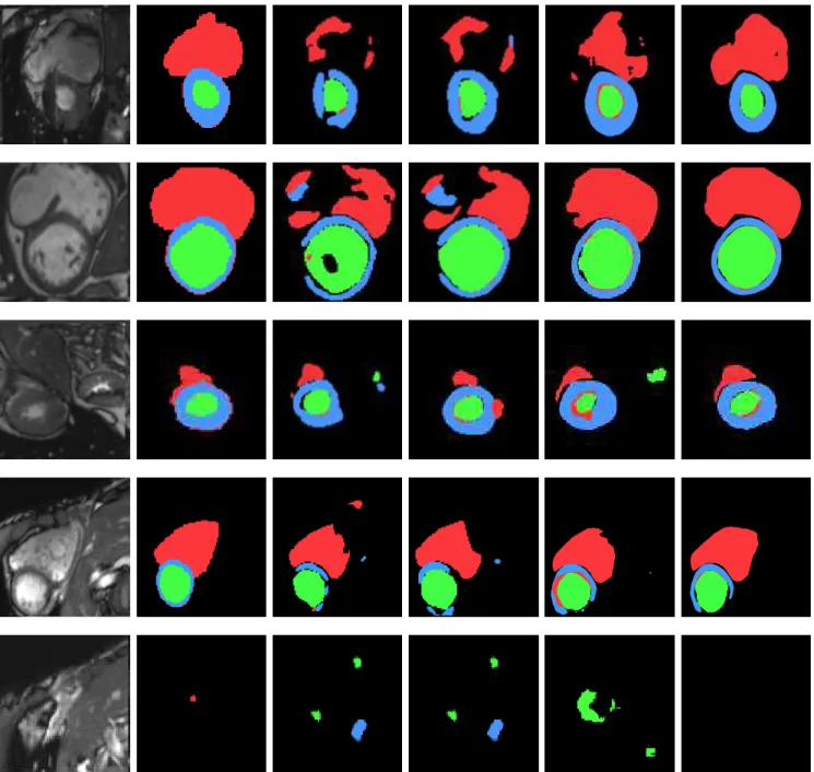
Figure 3: Segmentation results of left ventricle (red), right ventricle (green) and myocardium (blue) of five examples images using 2D U-Net and 2D Dense-Net with CE and our AC loss functions. From left to right, the example-original MR image, ground truth, segmentation results by U-Net+CE, U-Net+AC, Dense-Net+CE and Dense-Net+AC are shown respectively.
of distance between two contours and is defined as [23]:
DH(T, P) =max ( sup t∈T inf p∈Pd(T, P),psup∈P inf t∈T d(T, P) ) (14) whereT,P ∈ [0,1]m×n are the ground truth contour and
the predicted contour respectively,tandprepresent pixels
ofT andP,d(t, p)is Euclidean distance betweentandp.
5. Results
We implemented our networks using Keras 1.1.0 with Tensorflow_gpu 1.10 as backend. We trained our models until convergence by using the ADAM optimizer with a
learning rate of10−4. All the experiments were performed using an Intel CPU, and a NVIDIA TitanX GPU. Upon ac-ceptance of the manuscript, our trained models will be made available online at https://github.com/xuuuuuuchen/AC-loss. In Figure 3, segmentation results of left ventricle, right ventricle and myocardium of five examples images us-ing 2D U-Net and 2D Dense-Net with CE and our AC loss functions are displayed respectively.
5.1. Performance
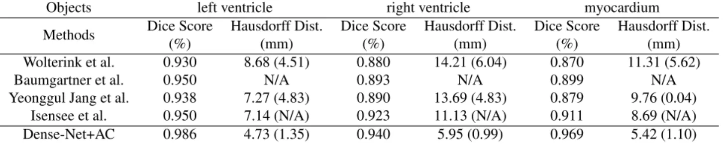
Table.1 showed the comparison results for the segmen-tation of left ventricle, right ventricle and myocardium between U-Net and Dense-Net when either CE or our AC loss function was used. The proposed approaches U-Net-AC has improved HD than U-Net-CE, so do Dense-Net+AC. As such we used the results of Dense-Net+AC for the comparative studies with previous studies. As shown in Table.1, our AC loss function based on Dense-Net (Dense-Net+AC) model achieves better results than others for all the segmentation tasks. The HD is 33.8%, 46.5% and 37.7% higher for the segmentation of left ventricle, right ventricle and myocardium respectively.
In Table.2, it presents that comparison with U-Net and Dense-Net with CE loss function and our AC loss function. In which, left ventricle, right ventricle and myocardium are listed at the top respectively. We use DC and HD for eval-uating the performance. The proposed approaches U-Net-AC, as well as Dense-Net+U-Net-AC, are compared against gen-eral segmentation frameworks: U-Net and Dense-Net with CE loss function. In Figure 4, the computing time per epoch for AC is 110s, shorter than CE at 121s, during training for DenseNet. For UNet, AC takes 15s while CE takes 17s. For testing, it takes almost the same time when the same network is used.
Figure 4: Running time per epoch for AC and CE loss func-tions within different models
5.2. Robustness Analysis
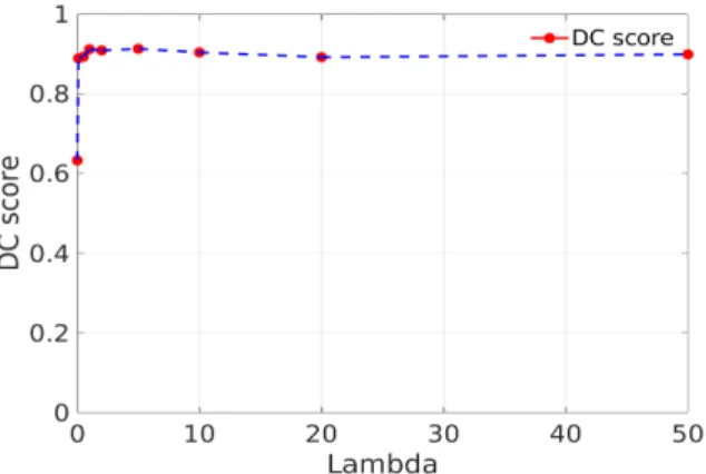
We evaluated the effect of the regularization weight λ in our AC loss function Eq.(8) by DC score. As shown in the Figure 5, our DenseNet-based model is robust to the choice of λ with differentλ values. When λ is close to zero, the DC result tends to be worse because only bound-ary term contributes to our loss function. We aslo evaluated the DenseNet-based model with region terms only under the same conditions compared with Dense-CE model. The per-formance (Dice Score) for this is 0.9634, worse than AC (0.9708) but better than CE (0.9442).
Figure 5: Effect of varying the parameterλon DC score
6. Discussion
Our proposed method AC loss function is able to take into account geometric information of the areas be segmented. We present two basic segmentation models U-Net and Dense-Net as a base to prove that our proposed loss function is robust in mainstream architectures. Our results also demonstrate that our model of loss function performs signicantly better than commonly used loss functions such as CE and DC when we test on a public MR ventricle dataset. Our results also demonstrate superior per-formance when compared to other start-of-art segmentation approaches. Compare to standard ACWE models which require iteration in solving PDEs, the use of CNNs have hugely reduced the computational time on new images although the training time will be longer.
We tested different values of the regularization weightλ to show this loss function is robust. In future work, we will investigate how to makeλcan be learned during the train-ing process. Similar to CE and DC that can be extended to multi-class segmentation problems [22], the proposed loss function can also be extended to solve multi-phase segmen-tation problems as the traditional ACM have demonstrated [32].
Table 1: Comparison with two different network: U-Net and Dense-Net on cardiac segmentation followed by CE loss function and our AC loss function. The three objects from cardiac MR scans (left ventricle, right ventricle and myocardium) are listed respectively. We use HD for evaluating the performance of segmentation. The proposed approaches U-Net-AC and Dense-Net+AC are compared against state-of-the-art segmentation U-Net and Dense-Net with CE loss function. Standard deviation is presented in the buckets respectively.
Objects left ventricle right ventricle myocardium Methods Hausdorff Dist.
(mm) Hausdorff Dist. (mm) Hausdorff Dist. (mm) U-Net-CE 18.29 (2.04) 23.76 (2.52) 18.04 (1.97) U-Net-AC 17.36 (2.76) 22.94 (2.48) 16.60 (2.05) DenseNet+CE 5.43 (1.81) 6.21 (1.05) 6.34 (1.56) DenseNet+AC 4.73 (1.35) 5.95 (0.99) 5.42 (1.10)
Table 2: Comparison with previous approaches on cardiac segmentation. In the top of table, the three objects (left ventricle, right ventricle and myocardium) are listed respectively. The accuracy is evaluated in terms of mean Dice Coefficient (DC) score and Hausdorff distance (HD). The proposed approach (Dense-Net+AC) is compared against state-of-the-art cardiac segmentation models: Wolterink et al. [30], Baumgartner et al. [2], Yeonggul Janget al. [11] and Isensee et al. [10]. Standard deviation is presented in the buckets respectively.
Objects left ventricle right ventricle myocardium
Methods Dice Score (%) Hausdorff Dist. (mm) Dice Score (%) Hausdorff Dist. (mm) Dice Score (%) Hausdorff Dist. (mm) Wolterink et al. 0.930 8.68 (4.51) 0.880 14.21 (6.04) 0.870 11.31 (5.62)
Baumgartner et al. 0.950 N/A 0.893 N/A 0.899 N/A
Yeonggul Jang et al. 0.938 7.27 (4.83) 0.890 13.69 (4.83) 0.879 9.76 (0.04) Isensee et al. 0.950 7.14 (N/A) 0.923 11.13 (N/A) 0.911 8.69 (N/A) Dense-Net+AC 0.986 4.73 (1.35) 0.940 5.95 (0.99) 0.969 5.42 (1.10)
7. Conclusion
In this paper, we introduced a new AC loss function that was inspired by ACMs for the segmentation tasks. The advantage of this new loss function is that it can seam-lessly combine the geometrical information (e.g. bound-ary length) with region similarity thus leading to more pre-cise segmentation. After implementation, we applied it to a large-scale CMR dataset and the results showed that the proposed approach outperforms state-of-the-art approaches. It is believed that this new development will be readily ap-plied to other challenging segmentation tasks posed by var-ious real applications.
References
[1] SM Masudur Rahman Al Arif, Karen Knapp, and Greg Slabaugh. Shape-aware deep convolutional neural network for vertebrae segmentation. InInternational Workshop and Challenge on Computational Methods and Clinical Appli-cations in Musculoskeletal Imaging, pages 12–24. Springer, 2017.
[2] Christian F Baumgartner, Lisa M Koch, Marc Pollefeys, and Ender Konukoglu. An exploration of 2d and 3d deep learn-ing techniques for cardiac mr image segmentation. In
Inter-national Workshop on Statistical Atlases and Computational Models of the Heart, pages 111–119. Springer, 2017. [3] Xavier Bresson, Selim Esedolu, Pierre Vandergheynst,
Jean-Philippe Thiran, and Stanley Osher. Fast global minimiza-tion of the active contour/snake model. Journal of Mathe-matical Imaging and Vision, 28(2):151–167, 2007.
[4] Tony Chan and Luminita Vese. An active contour model without edges. InInternational Conference on Scale-Space Theories in Computer Vision, pages 141–151. Springer, 1999.
[5] Pierrick Coupé, José V Manjón, Vladimir Fonov, Jens Pruessner, Montserrat Robles, and D Louis Collins. Patch-based segmentation using expert priors: Application to hippocampus and ventricle segmentation. NeuroImage, 54(2):940–954, 2011.
[6] Adrian V Dalca, John Guttag, and Mert R Sabuncu. Anatomical priors in convolutional networks for unsuper-vised biomedical segmentation. InProceedings of the IEEE Conference on Computer Vision and Pattern Recognition, pages 9290–9299, 2018.
[7] Jiu-lun Fan and Feng Zhao. Two-dimensional otsu’s curve thresholding segmentation method for gray-level images. Acta Electronica Sinica, 35(4):751, 2007.
[8] Ross Girshick. Fast r-cnn. InProceedings of the IEEE Inter-national Conference on Computer Vision, pages 1440–1448, 2015.
[9] Gao Huang, Zhuang Liu, Laurens Van Der Maaten, and Kil-ian Q Weinberger. Densely connected convolutional net-works. InProceedings of the IEEE Conference on Computer Vision and Pattern Recognition, volume 1, page 3, 2017. [10] Fabian Isensee, Paul F Jaeger, Peter M Full, Ivo Wolf, Sandy
Engelhardt, and Klaus H Maier-Hein. Automatic cardiac disease assessment on cine-mri via time-series segmentation and domain specific features. InInternational Workshop on Statistical Atlases and Computational Models of the Heart, pages 120–129. Springer, 2017.
[11] Yeonggul Jang, Yoonmi Hong, Seongmin Ha, Sekeun Kim, and Hyuk-Jae Chang. Automatic segmentation of lv and rv in cardiac mri. InInternational Workshop on Statistical At-lases and Computational Models of the Heart, pages 161– 169. Springer, 2017.
[12] Simon Jégou, Michal Drozdzal, David Vazquez, Adriana Romero, and Yoshua Bengio. The one hundred layers tiramisu: Fully convolutional densenets for semantic seg-mentation. In Computer Vision and Pattern Recognition
Workshops (CVPRW), 2017 IEEE Conference on, pages
1175–1183. IEEE, 2017.
[13] Michael Kass, Andrew Witkin, and Demetri Terzopoulos. Snakes: Active contour models. International Journal of Computer Vision, 1(4):321–331, 1988.
[14] Alex Krizhevsky, Ilya Sutskever, and Geoffrey E Hinton. Imagenet classification with deep convolutional neural net-works. InAdvances in Neural Information Processing Sys-tems, pages 1097–1105, 2012.
[15] Xiaomeng Li, Hao Chen, Xiaojuan Qi, Qi Dou, Chi-Wing Fu, and Pheng Ann Heng. H-denseunet: Hybrid densely connected unet for liver and liver tumor segmentation from ct volumes.arXiv preprint arXiv:1709.07330, 2017. [16] Tsung-Yi Lin, Priyal Goyal, Ross Girshick, Kaiming He, and
Piotr Dollár. Focal loss for dense object detection. IEEE Transactions on Pattern Analysis and Machine Intelligence, 2018.
[17] Geert Litjens, Thijs Kooi, Babak Ehteshami Bejnordi, Ar-naud Arindra Adiyoso Setio, Francesco Ciompi, Mohsen Ghafoorian, Jeroen Awm Van Der Laak, Bram Van Gin-neken, and Clara I Sánchez. A survey on deep learning in medical image analysis.Medical Image Analysis, 42:60–88, 2017.
[18] Wei-Chih Tu1 Ming-Yu Liu, Varun Jampani2 Deqing Sun Shao-Yi, Chien1 Ming-Hsuan Yang, and Jan Kautz. Learn-ing superpixels with segmentation-aware affinity loss. 2018. [19] Fausto Milletari, Nassir Navab, and Seyed-Ahmad Ahmadi. V-net: Fully convolutional neural networks for volumetric medical image segmentation. In 3D Vision (3DV), 2016 Fourth International Conference on, pages 565–571. IEEE, 2016.
[20] Anca Morar, Florica Moldoveanu, and Eduard Gröller. Im-age segmentation based on active contours without edges. In 2012 IEEE 8th International Conference on Intelligent Computer Communication and Processing, pages 213–220. IEEE, 2012.
[21] David Mumford and Jayant Shah. Optimal approximations by piecewise smooth functions and associated variational
problems.Communications on Pure and Applied Mathemat-ics, 42(5):577–685, 1989.
[22] Sérgio Pereira, Adriano Pinto, Victor Alves, and Carlos A Silva. Brain tumor segmentation using convolutional neu-ral networks in mri images. IEEE Transactions on Medical Imaging, 35(5):1240–1251, 2016.
[23] Javier Ribera, David Güera, Yuhao Chen, and Edward Delp. Weighted hausdorff distance: A loss function for object lo-calization.arXiv preprint arXiv:1806.07564, 2018. [24] Olaf Ronneberger, Philipp Fischer, and Thomas Brox.
U-net: Convolutional networks for biomedical image segmen-tation. InInternational Conference on Medical Image Com-puting and Computer-assisted Intervention, pages 234–241. Springer, 2015.
[25] Karen Simonyan and Andrew Zisserman. Very deep convo-lutional networks for large-scale image recognition. arXiv preprint arXiv:1409.1556, 2014.
[26] Christian Szegedy, Wei Liu, Yangqing Jia, Pierre Sermanet, Scott Reed, Dragomir Anguelov, Dumitru Erhan, Vincent Vanhoucke, and Andrew Rabinovich. Going deeper with convolutions. InProceedings of the IEEE Conference on Computer Vision and Pattern Recognition, pages 1–9, 2015. [27] Meng Tang, Abdelaziz Djelouah, Federico Perazzi, Yuri Boykov, and Christopher Schroers. Normalized cut loss for weakly-supervised cnn segmentation. InIEEE Conference on Computer Vision and Pattern Recognition (CVPR), Salt Lake City, 2018.
[28] Phi Vu Tran. A fully convolutional neural network for cardiac segmentation in short-axis mri. arXiv preprint arXiv:1604.00494, 2016.
[29] Luminita A Vese and Tony F Chan. A multiphase level set framework for image segmentation using the mumford and shah model. International Journal of Computer Vision, 50(3):271–293, 2002.
[30] Jelmer M Wolterink, Tim Leiner, Max A Viergever, and Ivana Išgum. Automatic segmentation and disease classifi-cation using cardiac cine mr images. InInternational Work-shop on Statistical Atlases and Computational Models of the Heart, pages 101–110. Springer, 2017.
[31] Yalin Zheng and Ke Chen. A hierarchical algorithm for mul-tiphase texture image segmentation.ISRN Signal Processing, 2012, 2012.
[32] Yalin Zheng and Ke Chen. A general model for multi-phase texture segmentation and its applications to retinal im-age analysis. Biomedical Signal Processing and Control, 8(4):374–381, 2013.
[33] Xiao-Yun Zhou, Mali Shen, Celia Riga, Guang-Zhong Yang, and Su-Lin Lee. Focal fcn: Towards small object segmentation with limited training data. arXiv preprint arXiv:1711.01506, 2017.