An Application of Linear Programming for Efficient Resource
Allocation
Onyekachi E. Wogu(Corresponding author) School of Postgraduate Studies, Benson Idahosa University
E-mail: [email protected]
Abstract
Every business organisation exits primarily to make profit while ensuring its continued existence. In a bid to maximise profit with the limited available resources, it becomes imperative therefore that efficient allocation be made of these resources. This paper ex-rays the concept of linear programming as an optimisation technique for maximising profit with the available resources. It goes further to address a problem encountered by a business (Eat Plaza)who due to an increment in price of raw material wants to strim- line its production. The linear programming model is used to analyse this problem and an optimum solution is reached as well as relevant recommendations to the management.
Keywords: linear programming model, limited resources, optimum, profit
1. Introduction
Every business enterprise strives to profitably exist while ensuring growth and expansion of its business endeavours. In its bid to achieve the above objectives it becomes expedient that critical decisions be made as regards allocation of its scarce resources effectively and also efficiently. These decisions includes but are not limited to, competitive price, identification of target market, product standard, level of technology involvement, manpower and so on. Owing to the fact that such decisions can become the make or break of the business thus distinguishing between a mediocre and an outstanding business.
It is important to note however that economic problems arise when available resources in organisations are not properly allocated or utilised [Akiniyi, .J.A, 2008]. It is a well known that a Nation’s economy is said to be buoyant when a lot of business within the country is thriving. This can be said as the reason why attempts are always being made by government to ensure measures are put in place to create an enabling external environment for businesses within their jurisdiction.
Every entrepreneur or business manager is faced with the challenge of decision making as regards efficient allocation of its available resources to various areas of need that pertains to the organisation. This above is in an attempt to minimize cost incurred while maximizing profit earned. Such resource allocation decisions can be facilitated and enhanced through the use of an operations research technique termed linear programming.
Linear programming is an optimisation instrument, which allows the rationalisation of many managerial and/or technological decisions. Linear programming is a technique designed to help operations managers plan and make decisions relative to the trade-offs necessary to allocate resources [Heizer, J andRender, B. 2004]. Linear programming is a method for the formalization and analysis of constrained optimization problems in which the objective function is a linear function and is to be maximized or minimized subject to a number of linear inequality constraints [Akiniyi, .J.A, 2008]
1.1Why Linear Programming Technique
[Agbadudu .B. A, 1996] Asserts that linear programming is a mathematical technique for finding the best uses of a firm’s or organizational limited resources. He further explained that it is a mathematical programming method for resolving problems associated with resource allocation.
Linear programming is a mathematical problem when the objective function as well as all the constraints are expressed by linear affine functions [Brandimarte .P, 2011]
Linear programming was aptly defined by [Dwivedi .N. D, 2003] as a technique for finding an optimum solution to the problem of resource allocation in order to achieve certain ends under the prescribed conditions.
Linear programming is a mathematical technique designed to assist management in solving optimisation problem when a decision has to be reached as to achieving the desired objective subject to limitations imposed in terms of restricted resources available, and/or desired quantities and/or qualities of output [Chartered Institute of management Accounting, 2009]. The author also asserts that allocation of scarce and limited resources amongst competing needs is a daily occurrence. There exist real life situations where linear programming comes handy in resource allocation which are but not limited to the following:
d) It is a useful tool for solving transportation problems, assignment problems with the aim of minimizing costs.etc.
1.1.1 Basic Assumptions of Linear Programming Model
. Components of a linear programming model have been identified by [Taha, A. H, 2011], [Bronson, .R, Naadimuthu, .G, 1997], [Stevenson .J.W, 2005], [Krajewski .J. L, Ritzman .P.L, Malhotra .k. M, 2007], [Dwivedi .N. D, 2008], [Hirschey .M, 2003] and [Budnick .S. F, Mcleavey .D, Mojena .R, 1988] as follows:
i. Proportionality: The level of activity is proportional to the contribution as well as consumption of resources.
ii. Additivity: Activities contribution and consumption are additive.
iii. Non-negativity: The values of the activities cannot be negative.
iv. Linearity: There exist linear relationships between the output of each product and the total quantity of
each resource consumed.
v. Single or one Objective function: There can be only one objective in a particular problem, either to maximise profit or to minimize cost not both.
vi. Certainty/ Deterministic: This presupposes that all values and quantities are known.
vii. Fixed external factors: This implies that the external environment is assumed not to vary.
1.1.2 Basic Components of a Linear Programming model
A linear programming usually is expressed in inequalities, below are the various component that make up an LP model, [Dwivedi .N. D, (2003)], [Krajewski .J. L,Ritzman .P.L, Malhotra .k. M, 2007], [Dwivedi, N.D, 2008], [Hirschey .M, (2003] and [Stevenson, J.W, 2009]:
a) Decision variables: e.g x1, x2
b) Objective function: e.g Min C = 12x1 + 10x2
c) Constraints/limitations: e.g available labour hours, machine hours
d) Non – negativity constraint.
1.1.3 Mathematical Statement of the Linear Programming Model Definition of symbols:
xj= jth decision variable.
cj= Coefficient on jth decision variable in the objective function. aij = Coefficient in the ith constraint for the jth variable.
bi = Right-hand-side constant for the ith constraint. n = Number of decision variables.
m = Number of structural constraints.
Based on the above definitions, the linear programming model can thus be stated as: Optimize (maximise or minimise)
z = c1x1 + c2x2 + . . . +cnxn
Subject to structural constraints
a11 x1 + a12x2+.. .+ a1n xn(≥)(≤)b1
a21 x1 + a22x2+... + a2nxn(≥)(≤) b2n
A =
am1x1+ am2x2+. . . + amnxn(≥)(≤) bm
x1,x2, . . ., xn≥ 0
The primary objective of this paper is to clearly show how a business organisation can efficiently allocate its limited resources amongst competing products or needs with the sole aim of concentrating its efforts on the highest yielding resource in terms of its contribution to profit generated. Having established a foundation on what linear programming is as well as state its general form, it becomes important to show its practical application in a business situation.
A fast food by name EAT PLAZA has a caterer that bakes meat pie, sausage and chicken pie. The owner wishes to know which of the above snacks to discontinue sales as a result of an increment in the price of flour and margarine. Expressed in table 1is the contributions made by each of the snacks and the quantity of materials
STEP 1: Convert the above problem to a linear programming problem standard form. Max π = 200x1 + 250x2 + 350x3 objective function
Subject to 500x1 + 250x2 + 500x3≤ 5000 flour constraint
250x1 + 100x2 + 200x3≤ 3000 margarine constraint
100x1 + 150x2 + 200x3≤ 8000 eggs constraint
x1, x2, x3≥ 0 non-negativity constraint
When the variables (xi) are more than two the SIMPLEX method becomes most appropriate in obtaining the
optimal solution, hence we shall be using the SIMPLEX method to solve this problem. STEP 2: Introduce slack variables in the constraints [Azimi, .M, et al, 2013]
500x1 + 250x2 + 500x3 + s1 + 0s2 + 0s3 = 5000
250x1 +100x2 + 200x3 + 0s1 + s2 + 0s3 = 3000
100x1 + 150x2 + 200x3 + 0s1 + 0s2 + s3 = 8000
x1, x2, x3, s1, s2, s3≥ 0
STEP 3: Introduce the slack variable in the objective function [Fagoyinbo, I. S,et al,2011] π = 200x1 + 250x2 + 350x3 + 0s1 + 0s2 + 0s3
π-200x1 – 250x2 -350x3 + 0s1 + 0s2 + 0s3 = 0 (the si symbols is not affected because 0
beingpositive or negative has no impact on its value) STEP 4: Draw the initial tableau
STEP 5: To identify the pivot row, divide the entire pivot column by the entire ‘b’ column (the right end column) and select the smallest value. The intersection between the pivot column and the pivot row is known as the pivot element (it is the foundation on which the next tableau is introduced).
The Gauss- Jordan row operation shall be applied in solving this linear programming problem (LPP) Where
R = Row Ȓ = New Row
R1(b) ÷ 500(x3 row 1) = 10 * pivot row
R2 (b) ÷ 200(x3 row 2) = 15
R3 (b) ÷ 200(x3 row 3) = 40
STEP 6: Draw a second tableau, introduce the pivot row into the slack variable (SV) where the pivot element was derived (x3) and divide each number in the entire row by the pivot element.
R1(b) ÷ 1/2(x2 row 1) = 20 * pivot row
R2 (b) ÷ 0 (x2 row 2) = ~ (infinity hence disregard)
R3 (b) ÷ 50 (x2 row 3) = 120
STEP 7: Since there is still a negative value (which indicates we have not reached optimum level) in the 4th row, we proceed to draw the third tableau following the same procedure.
The optimality condition of no negative value in the last column (π) has been meet hence this last tableau becomes the optimal.
In using the Gaussian row operation, we observe that the values under the pivot element must be manipulated to result in zero (0) in the next tableau drawn. This also serves as a check to ensure that the analysis is in order. Having no negative value in the last column is a signal that the optimum solution has been reached, thus bring the iteration to a halt and then evaluation is carried out on the values of the final (optimum) tableau. 1.1.4 Recommendations
Management can therefore engage the following solutions as they see fit given the findings derived from the analyzing the situation using SIMPLEX method:
1. Arbitrarily discontinue production of meat pie or chicken pie or both (meat pie and chicken pie) to concentrate on sausages.
2. Engage in staff training and ensure practical demonstrations of how to bake meat pie and chicken pie.
3. Check through the production system for possible lapses and take corresponding action.
4. Cease ordering for more stock of flour and margarine and harness the available resources
1.1.5 Conclusion
It has been clearly expressed from the above empirical data that resource allocation problems can be optimally and efficiently evaluated to enhance management decision making. It would have been difficult or impossible to know what to do with such statistics or data without skill application of optimisation model (in this case linear programming). As rightly indicated by [Taha, A. H 2011] there are computer softwares that enhance speed and accuracy in computing linear programming models such as Microsoft excel spread sheet, Riddy Ricks etc. These procedures were carefully outlined or explained to aid better understanding of how the optimum solution is generated using linear programming model.
It is important to express that the linear programming model is not without its limitations. [17]Some of which includes inability to predict prices, difficulty in accounting for diminishing marginal returns, its lack of operator risk preference, poor handling of decreasing cost. The above limitations not withstanding do not detract from its importance and usefulness as an optimisation technique.
References
Agbadudu .B. A, (1996). Elementary Operations Research, vol 1, Benin: A.B Mudiaga.
Akiniyi, .J.A, (2008). Allocating available resources with the aid of linear programming: roadmap to economic recovery, Multidisciplinary Journal of Research development, 10(2), 113-139.
Azimi, .M, Beheshti, .R.R, Imanzadeh, .M, Nazari, .Z, (2013). OptimalAllocation of HumanResources by Using Linear Programming in the Beverage Company, Universal Journal of Management and Social Sciences, 3 (5), pp 48 – 54.
Brandimarte .P, (2011). Quantitative Methods: An introduction for business management, New Jersey: John Wiley & Sons.
Bronson, .R, Naadimuthu, .G, (1997). Schaum’s outlines Operations Research, 2ndedUS: McGraw- Hill.
97 – 105.
Ferguson, S.T, Linear Programming: a concise introduction (n.d)
Heizer, J, Render,B,(2004). Operations Management, 7thed, (New Jersey: Pearson Prentice-Hall.
Hirschey .M, (2003). Fundamentals of Managerial Economics, 7thed, Ohio: Thompson South- Western.
Krajewski .J. L, Ritzman .P.L, Malhotra .k. M, (2007). Operations Management: Processes and Value Chains, 8thed, New Jersey: Prentice-Hall.
Meeks, A. T, (2002). A linear programming analysis of profitability and resource allocation among cotton and peanuts considering transgenic Seed technologies and harvest timeliness, A Thesis Submitted to the Graduate Faculty of The University of Georgia in Partial Fulfillment of the Requirements for the Degree Masters of Science Athens, Georgia.
Stevenson .J. W, (2009). Operations Management, 10thed, New York: McGraw –Hill/ Irwin.
Stevenson .J.W, (2005). Operations Management, 8thed, New Delhi: Tata McGraw-Hill.
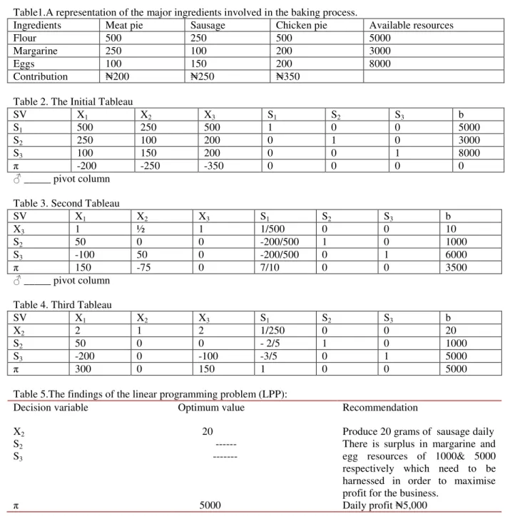
Taha, A. H, (2011). Operations Research: an introduction, 9thed, New Jersey: Pearson Prentice-Hall, 2011. Table1.A representation of the major ingredients involved in the baking process.
Ingredients Meat pie Sausage Chicken pie Available resources
Flour 500 250 500 5000
Margarine 250 100 200 3000
Eggs 100 150 200 8000
Contribution ₦200 ₦250 ₦350
Table 2. The Initial Tableau
SV X1 X2 X3 S1 S2 S3 b S1 500 250 500 1 0 0 5000 S2 250 100 200 0 1 0 3000 S3 100 150 200 0 0 1 8000 π -200 -250 -350 0 0 0 0 ♂ _____ pivot column
Table 3. Second Tableau
SV X1 X2 X3 S1 S2 S3 b X3 1 ½ 1 1/500 0 0 10 S2 50 0 0 -200/500 1 0 1000 S3 -100 50 0 -200/500 0 1 6000 π 150 -75 0 7/10 0 0 3500 ♂ _____ pivot column
Table 4. Third Tableau
SV X1 X2 X3 S1 S2 S3 b
X2 2 1 2 1/250 0 0 20
S2 50 0 0 - 2/5 1 0 1000
S3 -200 0 -100 -3/5 0 1 5000
π 300 0 150 1 0 0 5000
Table 5.The findings of the linear programming problem (LPP):
Decision variable Optimum value Recommendation
X2 20 Produce 20 grams of sausage daily
S2
S3
--- ---
There is surplus in margarine and egg resources of 1000& 5000 respectively which need to be harnessed in order to maximise profit for the business.