User-Assisted Image Shadow Removal

User-Assisted Image Shadow Removal

Han Gonga,∗_{, Darren Cosker}b

a_{School of Computing Sciences, University of East Anglia, Norwich, UK} b_{Department of Computer Science, University of Bath, Bath, UK}

Abstract

This paper presents a novel user-aided method for texture-preserving shadow removal from single images requiring simple user input. Compared with the state-of-the-art, our algorithm offers the most flexible user interaction to date and produces more accurate and robust shadow removal under thorough quantitative evaluation. Shadow masks are first detected by analysing user specified shadow feature strokes. Sample intensity profiles with variable interval and length around the shadow boundary are detected next, which avoids artefacts raised from uneven boundaries. Texture noise in samples is then removed by applying local group bilateral filtering, and initial sparse shadow scales are estimated by fitting a piecewise curve to intensity samples. The remaining errors in estimated sparse scales are removed by local group smoothing. To relight the image, a dense scale field is produced by in-painting the sparse scales. Finally, a gradual colour correction is applied to remove artefacts due to image post-processing. Using state-of-the-art evaluation data, we quantitatively and qualitatively demonstrate our method to outperform current leading shadow removal methods.

Keywords: image shadow removal, user-assisted computer vision, colour correction, curve fitting, smoothing.

2010 MSC: 68U10, 68U05

1. Introduction

Shadows are ubiquitous in natural scenes, and their re-moval is an interesting and important area of research. As well as a motivation to solve this problem for artistic image editing, shadows can affect the performance of many com-5

puter vision algorithms. For example, unwanted shadow boundaries can cause artefacts in image segmentation and contribute to drift when tracking given moving objects and scenes.

In this paper, a semi-automatic method is proposed 10

for high-quality shadow removal using user-defined flexi-ble single strokes covering the shadow and lit pixels. Our method sacrifices full autonomy for extremely simple user

∗_{Corresponding author}

Email addresses: [email protected](Han Gong), [email protected](Darren Cosker)

input, as opposed to existing manual approaches that re-quire fine-scale input,e.g.accurate shadow contours. Given 15

detection, our method produces accurate shadow removal optimised for robust penumbra recovery. Using the current state-of-the-art shadow removal ground truth dataset [1], our solution is quantitatively evaluated against other lead-ing methods and demonstrates notably improved perfor-20

mance. Numerous visual comparisons of our method ver-sus existing methods are also presented, demonstrating qualitatively more pleasing results. Our approach repre-sents what we believe to be a state of the art technique for shadow removal with a thorough evaluation against the 25

current leading approaches.

1.1. Related Work

A shadow generally consists of an umbra and penum-bra area. The umpenum-bra is the darkest part of the shadow

while the penumbra is the wide outer boundary with a gradual intensity change between the umbra and lit area. The penumbra scale is non-uniform and shadowed surface textures generally become weaker within it. A shadow im-ageI+

c can be considered to be a Hadamard product of a

shadow scale layer_Scand a shadow-free imageIc∗as shown

in Eq. 1.

I_c+=I_c∗_{◦ S}c (1)

For a lit pixel, the illumination is constant in both shadow and shadow-free images. For a shadow pixel, its intensity in a shadow image is lower than its intensity in the shadow-30

free image. Consequently, the scales _Sc of the lit area are

1 and other areas’ scales are between 0 and 1.

However, most images appearing on the Internet are not linear images. These images have commonly been post-processed by some non-linear image processing algo-35

rithms such as gamma-correction, JPEG compression, and non-linear filters. After a linear shadow recovery process, contrast artefacts can appear in the shadow areas [2].

Approaches to shadow removal can be categorised as either automatic [1, 3–8] or user-aided [2, 9–11]. The prob-40

lem can be broken down into two stages: shadow detection and shadow removal.

Automatic approaches do not require any user interac-tion but risk inaccurate shadow detecinterac-tion or require spe-cial setups for capture which do not work for general im-45

ages. Intrinsic image based methods are a popular branch of automatic techniques (e.g. [3, 4]). The decomposition of intrinsic images provides shading and reflectance infor-mation but can be unreliable leading to over-processed results. The decomposition is generally based on an as-50

sumption that the illumination change is smooth or the refectances of the scene lies on an illumination-invariant direction. Another branch of techniques are shadow fea-ture learning based methods [1, 12–16]. However, detec-tion can be often unreliable due to limited training data 55

and the quality of initial image edge detection and seg-mentation. Several approaches [12–14, 16] detect shadows

by classifying edges in images using edge features,e.g. in-tensity, texture, chromaticity and intensity ratio. Graph-ical models [1, 15] can also form the basis of detection. 60

Yao et al. [15] detect shadow by using a reliable graph model and colour features to classify pixels. In their ap-proach, each pixel is a node with encodes node reliability based on strength of shadow feature, and node relation-ships described using similarity between neighbours. Guo 65

et al.[1] detect shadows by classifying segments in images that adopt similar shadow features and remove shadows using a variant alpha-matting algorithm. Some methods apply additional active light sources to capture shadowless objects, e.g., by comparing images with an illumination 70

source at different positions [5] and comparing flash and no-flash image pairs [6]. However, active lighting restricts the types of scene that shadow removal can be applied to – as using special lighting setups outdoors is often not prac-tical. Other methods adopt optical filters to acquire multi-75

spectral information to achieve illumination detection,e.g.

by comparing NIR and RGB images [7] and by compar-ing RGB and scompar-ingle-colour-filtered images [8], but these methods are generally limited to special scenario cases,

e.g.sunlight and non-black surfaces. 80

User-aided methods generally achieve better shadow detection and removal at the cost of user input. Wu et al.[9] require a high degree of user intervention where mul-tiple regions of shadow, lit area, uncertainty and exclusion are identified. They apply a Bayesian optimisation to de-85

rive a shadow matte and a shadow-free image. Others [10, 11] require fine input defining the shadow boundary. Liu and Gleicher [10] proposed a curve fitting method and a global alignment of gradients to acquire shadow scales but have issues when relighting the umbra and can introduce 90

artefacts at uneven boundaries. Shor and Lischinski [17] detect shadow using image matting from a grown shadow seed. They only require one shadow pixel as input, but have limitations in cases where the other shadowed sur-faces are not surrounded by the initially detected surface 95

or when the penumbra is too wide. Arbel and Hel-Or [2] apply a thin-plate model to the intensity surface. They require users to specify multiple texture anchor points to detect the shadow mask but the input overhead increases when shadows are distributed in multiple regions. Su and 100

Chen [11] developed a method to estimate shadow scales using dynamic programming. Their gradient alignment for intensity samples allows for less accurate user inputs compared with [9, 10]. They also provide a healing tool for users to manually amend artefacts in highly-curved 105

shadow boundary segments. Gong and Cosker [18] intro-duced a fast approach which categorises intensity profiles into several sub-groups and derives the shadow scales for each of them. They require two types of scribbles for mark-ing lit and shadow pixels. Similarly, Zhang et al. [19] re-110

quire the same user input of [18].However, their method requires a shadow matte (guided by the user’s scribbles) to identify shadows, which is sensitive to user-scribbles be-cause their image matting is affected by pixel location.

To date, most shadow removal methods [2, 9–11, 19] 115

have only been evaluated by visual inspection on some selected images – with only a few exceptions performing quantitative evaluation. Guo et al. [1] provided the first public ground truth data set for shadow removal and per-form quantitative testing. However, their error measure-120

ment is variant to the size and darkness of shadows and some of their shadow-free ground truth shows inconsis-tent illumination compared with the lit area of their cor-responding shadow images.

1.2. Contributions

125

Given our overview of state of the art approaches, 3 main contributions are proposed:

1) Simple user input: Past work, e.g. [2, 9–11], re-quires precise user-input defining the shadow boundary. Our method only requires users to define some single rough 130

strokes covering related shadow and lit pixels – without the need to differentiate between samples in shadow and

lit areas.

2) Intelligent sampling: Adaptive sampling with vari-able intervals and lengths is proposed to address shadow 135

boundary artefacts in past work [2, 10], which uses fixed intervals and lengths. Unlike past work [2, 10, 11], unqual-ified samples are intelligently filtered. These can affect the quality of shadow scale estimation,e.g.samples with high noise or sampling lines passing through boundaries caused 140

by occlusions or strong background texture.

3) Robust scale estimationFast local group processing is proposed for selected samples and initially estimated scales to improve smoothness of shadow removal. Post-processing effects cause inconsistency in shadow corrected 145

areas compared with the lit areas both in tone and con-trast. Without introducing chromatic artefacts, colour-safe correction is proposed to amend the scales.

To summarise, the paper presents several solutions to improve shadow removal quality, and these have been quan-150

titatively verified using robust error measurement and the standard data set in this area [1].

2. User-Assisted Image Shadow Removal

In this section, our algorithm is first described in brief before being expanded on with technical details for each 155

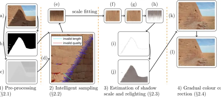
of its components. Our algorithm consists of 4 steps (see Fig. 1):

1) Pre-processing (§2.1) A shadow mask is detected (Fig. 1 (b)) using a KNN classifier trained from K-Means clustered data from user inputs (e.g. Fig. 1 (a)). A

fu-160

sion image is generated, which provides an illumination-insensitive layer, by fusing the channels of YCrCb colour space and de-noising (Fig. 1 (c)).

2) Intensity sampling (§2.2)Intensity profiles are ob-tained for sampling lines perpendicular to shadow bound-165

aries. Poor samples are filtered based on similarity of il-lumination change (Fig. 1 (d)) and de-noised using direc-tional bilateral filtering (Fig. 1 (e)).

(a)

(b)

(c)

1) Pre-processing

(

_§

2.1)

invalid length invalid quality

(d)

(e)

(f)

(g)

(h)

2) Intelligent sampling

(

_§

2.2)

scale fitting

(i)

(j)

3) Estimation of shadow

scale and relighting (

_§

2.3)

(k)

(l)

4) Gradual colour

cor-rection (

_§

2.4)

Figure 1: Shadow removal pipeline. (a) input: a shadow image and user strokes in white covering both shadowed and lit pixels; (b) detected shadow mask; (c) fusion image; (d) initial penumbra sampling: the blue lines are valid samples, the other lines are invalid samples. The original single stroke has been divided into lit (red) and shadow (blue) parts; (e) boundary image of samples; (f) re-lit and filtered boundary image; (g) re-lit boundary image after boundary artefact removal; (h) rectified shadow scale of boundary image (each column refers to the scales for a sample); (i) sparse shadow scales; (j) dense shadow scales; (k) initial shadow-free image; (l) colour-corrected shadow-free image.

Given the filtered intensity samples, these are fit through 170

and relit (Fig. 1 (f)) using a piece-wise cubic curve and a boundary image of the samples (Fig. 1 (e)). Any remain-ing boundary artefacts are removed usremain-ing directional scale suppression (Fig. 11(g)) over the boundary image. Fitted sparse scales are propagated (Fig. 1 (h-i)) to generate a 175

dense scale field (Fig. 1 (j)). Shadows are then removed (Fig. 1 (k)) by inverse scaling using this dense scale field.

4) Gradual colour correction (§2.4) Any remaining shadow removal artefacts due to image post-processing are finally treated with our colour correction (Fig. 1 (l)). 180

This uses statistics around penumbra boundaries and the shadow scale field.

2.1. Pre-processing

Pre-processing provides a shadow mask and a fusion image to assist intensity sampling (§2.2). Determining 185

the initial shadow mask is the first step of shadow re-moval and is required in many previous methods including [1, 2, 10, 18, 19]. Although some methods can achieve au-tomatic shadow detection, these results are dependent on

the quality and variation of training data. In this work, all 190

that is required is the user to supply single strokes covering related shadow and lit pixels (Fig. 1 (a)) – the remaining differentiation and recognition is fully automatic. Under many circumstances, our interaction is easy to perform as it does not require users to explicitly distinguish between 195

shadow and lit pixels. The pixels covered by the single user stroke are first classified as either shadow or lit pixels using K-Means clustering [20]. K-means is applied for this task because it is unsupervised and no training samples for differentiating shadow and lit pixels are provided by a user. 200

The feature used for clustering is the normalised RGB in-tensity and the normalised pixels coordinates. The cluster with the lowest mean for its RGB intensity is considered as a shadow cluster and vice versa. The classified input pixels’ RGB intensities are used as the training features 205

to construct a KNN classifier [21] (number of neighbours: 3). Euclidean distance is used as the distance measure and the majority rule with nearest point tie-break as the classification measure. KNN is applied for this task as it is a supervised algorithm that divides data entries into 2 210

clusters. The input image can be binarised as a shadow mask,e.g.Fig. 1 (b), using the pixel-wise KNN classifier. We adopt a fusion image [18] for assisting intensity sample collection. The fusion image provides an illumination-insensitive layer, e.g. Fig. 1 (c). It can be obtained by linearly fusing the channels of YCrCb colour space. The fused image _Fp is computed as a weighted sum of the 3

normalised channelsCl as follows:

Fp = ( 3 X l=1 Clϕ(σl))/( 3 X l=1 ϕ(σl)) (2)

wherel is the channel index,σlis the standard derivation

of the umbra sample intensities of _Cl. ϕ is an

exponen-tial incentive function for determining the weight for each channel.

ϕ(x) =x−5 (3)

wherexis the pixel intensity. Lower variation of intensity is preferred as it means higher intensity uniformity in the umbra segment. To suppress texture noise, a median fil-215

ter [22] with size h1 (default: 10) filter window is further

applied to_Fp.

2.2. Intensity Sampling

Our intensity sampling rejects inferior intensity sam-ples for robust shadow scale estimation. There are 3 steps:

1) Adaptive raw intensity sampling RGB intensity profiles are extracted along sampling lines perpendicular to the shadow boundary,e.g.Fig. 1 (d), where the boundary is obtained from the shadow mask. To accelerate shadow scale estimation, sampling lines are not measured at each shadow boundary point. Sparse and fixed distance sam-pling intervals are also avoided, as this may cause arte-facts at highly uneven boundary segments [2, 10]. Instead, smaller sampling intervals are adaptively assigned at seg-ments along the shadow boundary based on curvature. Our intention is to sample more intensity samples for curve shadow boundary segments. We compute a curvature ar-rayCwhich stores the curvatures of all shadow boundary points. A sampling mark is set for shadow boundary point

when its normalised absolute curvature is greater than a threshold h2 (default 0.05) as shown in the first case of

Eq. 4. Dm=                          1, |Cm| PN i=1|Ci| > h2 1, m= 1 or m=N 1, 4 X i=1 Dm−i= 0 0, Otherwise (4)

where N is the number of boundary points, m specifies the index of boundary points,Dis the sampling mark ar-220

ray. Themth _{shadow boundary point is set for sampling}

ifDm= 1. To provide enough intensity samples for image

borders, the first and last boundary points are also set for sampling (second case in Eq. 4). If the boundary is nearly straight, the sampling interval for that segment is fixed to 225

a maxima h3 (default: 5) as shown in the third case of

Eq. 4. As shown in Fig. 2, our variable sampling interval avoids penumbra removal artefacts around sharp bound-ary segments.

To adapt the variance of penumbra softness, the length of 230

a sampling line is guided by the fusion image. This prob-lem is equivalent to finding the locations of the two ends of a sampling line. A bi-directional search [18] is applied from each boundary point towards the lit area (end point) and the shadow area (start point) as described in Algo-235

rithm 1. The start and end points are initially set as the boundary pointpb. To get the position for a start point,

the boundary normalnbis iteratively subtracted from the start point (vice versa for the end point) until the average of two ends’ projected gradient strength (_Ls and Le) is

240

small enough (controlled by an attenuation factorh4with

a default value 5) or either of the ends is outside the range of image coordinates.

2) Intensity sample selection Outlier intensity sam-ples,e.g.Fig. 1 (d), can affect accurate shadow scale esti-245

mation and cause unnatural shadow removal results. Two criteria are adopted for outlier detection: a) Length of

(a) fixed interval 1 (b) fixed interval 2 [10] (c) variable interval

(d) original (e) fixed 1 (f) fixed 2 [10] (g) variable

Figure 2: Comparison of sampling scheme. The white lines in (a), (b), and (c) are the sampling lines of the fixed interval using boundary-perpendicular sampling, the fixed interval using horizontal/vertical sampling in [10], and our boundary-boundary-perpendicular variable interval sampling respectively. (d) is the original image. (e), (f), and (g) are the corresponding shadow removal results of the three sampling methods respectively.

Algorithm 1:Sample End-Point Selection

input : boundary point pb, boundary normal nb, fusion imageFp

output: two ends (ps,pe) of a sampling line

e F _{←− ∇F}p;L ←−Fe(pb)·nb; ps←−(pb);pe←−(pb); repeat vs_←−F([e ps]);ve←−Fe([pe]); Ls←−vs·nb;Le←−ve·nb; ps_←−ps₋nb;pe_←−pe+nb;

untileitherps orpe is outside_Fp or

h4(Ls+Le)<L;

sampling line. The minimum length of a sampling line is 3 and the maximum length is lµ + 3lσ where lµ and

lσ are the mean and the standard derivation of sample

250

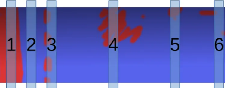
length respectively. The samples whose lengths are out of this range are removed; b) Similarity of illumination changes. Outliers of intensity samples are often caused by surface texture and such samples can affect illumination change estimation. Fig. 3 shows a synthetic example of 255

various intensity samples which better explains our mo-tivation. A rough RGB intensity profile is obtained by down-sampling each intensity sample to 3 pixels’ long us-ing discrete cosine transform (DCT) [23]. This short in-tensity profile is useful to cancel out texture noise. To 260

obtain the features of illumination change, this short in-tensity profile is converted to the Log-domain because the multiplicative shadow scales (Eq. 1) become additive in the Log-domain. The approximate derivatives for each chan-nel of each Log-domain intensity sample are supplied as 265

illumination change features. This results in a 6-D feature vector for each intensity sample (two derivatives for each RGB channel). We assume that the majority of illumina-tion change features are close to each other and can form a major cluster. The objective here is to find out the major 270

cluster and discard the other minor clusters. A density-based DBSCAN clustering method [24] (radiush5: 0.2) is

used to categorise the samples. The samples belonging to the largest cluster are identified as the samples with valid illumination change and the remaining invalid samples are 275

discarded. DBSCAN is chosen for this task as it does not constrain the number of clusters which is suitable for the fact that many outliers are often located in uncertain num-ber of smaller clusters distant to each other.

3) Sample de-noising Texture noise can still affect 280

the smoothness of shadow scale estimation even when the outliers are removed. Texture noise is removed from the selected intensity samples using a directional (i.e.parallel to normals of the shadow boundary) bilateral filter [25]. To achieve this, the raw intensity samples are first re-285

1 2 3

4

5

6

Figure 3: Intensity sample selection example. The 6 marked trans-parent blue lines are intensity sampling lines. Samples 1, 2, 5, 6 are classified as valid and the rest are invalid. Although the surface materials of sample 1 and 2 are different, their illumination change vectors are exactly the same and they both reflect true illumination change. This is because for each of them, the surface material in the shadow and lit areas are constant. Samples 3 and 4 are classified as outliers because the surface materials in the shadow and lit areas are varying. Sample 5 and 6 contain some varying surface materials, but the variations of the surface material are not significant. Therefore, they are still classified as valid samples.

sized as individual columns and their lengths are set as the maximum length of all raw samples. These columns are concatenated horizontally to form a boundary image,

e.g. Fig. 1 (e). A bilateral filter [25] is applied to each RGB channel of this image to suppress texture noise. A 290

Bilateral filter is chosen for this task as it removes texture noise and preserves edge and smooth intensity change.

2.3. Estimation of Shadow Scale and Relighting

This sub-section explains the procedure for removing shadows based on the processed intensity samples. The following description of the algorithm is applied to the samples of each detected shadow boundary. There are 3 steps:

1) Initial intensity fitting Having obtained filtered and resized intensity samples at different positions along the boundary, our goal is to find illumination scaling values in-side the umbra, penumbra and lit area. The shadow scale change functionS for each RGB channel of each intensity sample is modelled as follows (see also Fig. 4):

S(x) =            K 0_≤x_≤x1 f(x) x1< x≤x2 1 x2< x≤1 (5) K 1 x1 x2

Umbra Penumbra Lit

Figure 4: Shadow scale model:x1andx2define the ends of a

penum-bra region. Kis a scale of umbra intensity scale.

where x is a normalised pixel location within the sam-pling line, x1 and x2 determine the start and end of the

penumbra area respectively, andKis a positive scale con-stant for sample points within the umbra area (x < x1).

The constant 1 is assumed for the lit area piece (x > x2)

as this falls inside a lit area of the image and does not require re-scaling. The functionf is parametrised by K, v1 andv2 as follows:              f(x) = (1₋K)B(v1(x−v2)) +K B(y) =₋2y3_{+ 1.5y} −0.5 x1 x2 =v2+v1−1 −0.5 0.5 (6)

where B is a cubic shape function (a sinusoidal function here also produces adequate results) and y is the input, 295

v1 and v2 are two parameters used to define the shape of the illumination change function and are linearly re-lated to x1 and x2. Illumination of each channel usually varies differently (e.g.outdoor shadows appear bluish) and therefore 3 independent K (in Eq. 5) are estimated for 300

each channel. B is a smooth curve with two zero 1st_order

derivatives at both ends, which serves as a rough fit to the intensity change and helps to locate the penumbra loca-tion. Penumbra boundaries of the 3 channels are usually the same. Consequently, a common penumbra width and 305

position is assumed for each channel, determined by v1

andv2 respectively. This assumption of channel-invariant

penumbra location can make the optimisation more ro-bust. This is because the intensity sample of one channel can be very noisy but the others’ are not. In summary, for 310

each sampling line, there are 5 parameters to solve in total. The parameters can be solved by least squares fitting with

a sequential quadratic programming algorithm [26]. The fitted parameters of all sampling lines are also smoothed by using a robust smoothing method (maximum iteration: 315

100, weighting function: bi-square) [27].

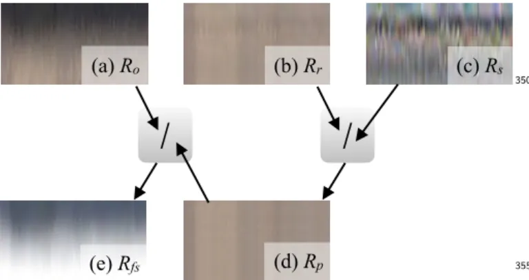
2) Boundary artefact removalFor some over-processed images, directly relighting the sparse samples using the fitted shadow scales may cause band-like artefacts in the penumbra. Directional scale suppression (Fig. 1 (f-h)) is 320

therefore applied. Fig. 5 shows an example of more obvious boundary artefact removal. The band artefacts appear as a

/

(a) Ro (b) Rr (c) Rs

(e) Rfs (d) Rp

/

Figure 5: Boundary artefact removal pipeline. (a) The boundary frame imageRo. (b) Initial re-lit imageRr. (c) The band-like arte-fact image Rs extracted from Rr. Rs is visualised in the log do-main. (d) Band-like artefact removed frame imageRp. (e) Amended shadow-scale frame imageRf s.

pattern in each re-lit intensity profile (Fig. 1 (b)). To sup-press these, the previously re-sized and filtered intensity profile is first aligned according to the estimated penum-325

bra position (x1 and x2) so that the illumination change

of each resized sample is synchronised. The concatenated boundary image is denoted as Ro. The boundary image

Ro is re-lit by inverse scaling according to Eq. 1 and the

resulting image is termedRr. It is assumed that band-like

330

artefacts are locally similar and a local group sizeh6= 5

is specified for suppression. To extract the local band pat-tern, horizontal filtering is applied toRrusing an average

kernel (size: 5x1) and the filtered image denoted asRf. To

suppress the band-like artefact, the variance of each col-335

umn’s, i.e.each samples, intensities ofRf are minimised.

To achieve this, a variance image Rs is computed by

di-viding each column’s intensities ofRf by its corresponding

average intensity of that column. The artefact-free and re-lit boundary image is computed as Rp =RrRs where

340

is an operator for element-wise division. Finally, the rectified scale image is computed asRf s=RoRp. The

sparse scales for each sampling lines corresponds to each column ofRf s.

3) RelightingTo obtain a dense scale field (e.g. Fig. 1 345

(j)), the sparse scales in the penumbra region are processed by smoothly interpolating and extrapolating the scales in other regions by using a general image in-painting algo-rithm [28]. Our adaptive intensity sampling (_§2.2) pro-vides enough shadow scale samples, in sub-pixel accuracy, 350

for recovering dense shadow scales in the curve shadow boundaries by using in-painting. The shadow-free image (e.g. Fig. 1 (k)) can be obtained by inverse scaling accord-ing to Eq. 1. As the dense shadow filed is formed by prop-agating the shadow scales in penumbra, a wrong shadow 355

scale estimate of a sampling line can produce wrong dense scales for a wider region. Our previous efforts in filtering bad intensity samples are thus crucial for this step.

2.4. Gradual Colour Correction

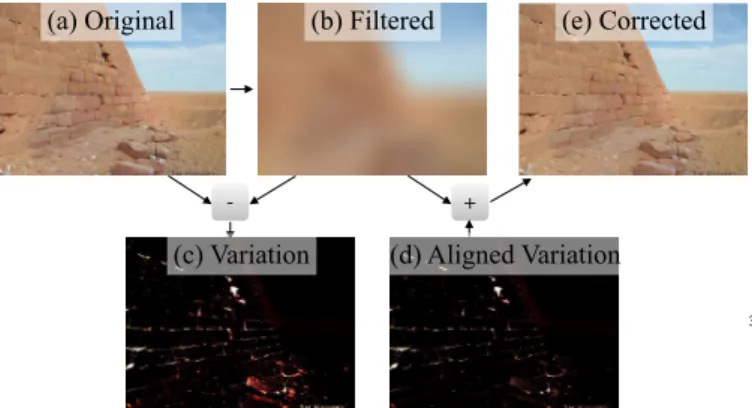
Some input images may have been significantly post-processed,e.g.through JPEG compression or gamma cor-rection. Highly visible artefacts, e.g. differences in tone and contrast, may appear in shadow corrected areas as Eq. 1 does not hold in such cases. To address this, a sim-ple gradual colour correction is introduced which is gener-ally compatible for unknown post-processing affects. This step is only necessary for over post-processed images and the difference may otherwise be insignificant for the other images. The shadow removed image is first converted to L*a*b* colour space because L*a*b* colour space is de-signed for visual perception adjustment [29]. It is assumed that the L*a*b* intensity variation of lower frequency is accurate and the errors appear in the intensity variation of higher frequencies. Fig. 6 shows the intermediate steps

(c) Rs

- +

(a) Original (b) Filtered

(c) Variation (d) Aligned Variation (e) Corrected

Figure 6: Gradual colour correction pipeline. The initial shadow-removed image (a) exhibits inconsistency between originally-lit and shadow-removed areas. This image is filtered (b) and used to extract an image of higher-frequency variation (c). The variation of shadow and lit areas are aligned. In (d), the original higher variation in the shadow area is made consistent (i.e. suppressed) with the lit areas’. The colour-corrected image is computed by adding (b) and (d). The variation images (c, d) are displayed by applying a gamma 3 to magnify the difference.

of colour correction in corresponding to the result in Fig. 1 (l). Statistics are collected from the lit side pixels Pl and the umbra side pixelsPu both near penumbra as the tar-get and source of colour correction respectively. Ps de-fines the set of all shadow pixels which include both um-bra and penumum-bra pixels,i.e.,Pu_⊂Ps. In L*a*b* colour space, the image of higher frequency intensity variation Ih _{= I}r

−Il _{is computed where I}l _{is the initial shadow}

removed imageIr_{filtered by a bilateral filter [25]. The}

ad-justment is completed in L*a*b* colour space as described in Eq. 7.      rσ =ς(Ich(Pl))/ς(Ich(Pu)) Ira c (Ps) =Icl(Ps) +rσIh(Ps) (7)

where c is the channel index, Ira is the colour corrected 360

image and the intensities of other unmodified pixel ofIra are identical to those ofIr, Ps is the set of all shadowed pixels,ς is a function computes the median absolute devi-ation.

Since our colour correction is only applied to the entire shadow segment, some minor intensity discontinuities may appear in the shadow boundary after colour correction. To smooth the colour correction result, an alpha blending is

applied in RGB colour space according to the shadow scale as the follows Icf =I r c ◦S˙c+Icra◦(1−S˙c) (8) ˙ Sc( ˙x,y) = max˙ Sc( ˙x,y)˙ −Sc5% 1−S5% c ,0 (9)

wherec is the channel index,xandy are the image coor-365

dinates,_Sw _{is the normalised scale field of}

S, S5% c is the

5% percentile of the values in ˙_Sc, Icf is the final

shadow-free image. The 5% percentile value is used for shadow scale normalisation instead of the minimum value because sometimes the minimum value can be an outlier distant 370

to the main cluster of a shadow scale distribution. The maximum operation ensures that the normalised shadow scale values are always non-negative. An example of this alpha-blending effect is shown in Fig. 7.

Initial Removal

Colour-Corrected

Figure 7: The colour-corrected image is blended with the initial shadow removed image. The resulting blend avoids intensity discon-tinuity at the shadow boundary. The zoom-in patches are makred by two grey boxes above. A visible crack-like boundary discontinuity is found in the middle of the left patch.

2.5. Customisable Parameters

375

In Tab. 1, we summarise the important parameters which users can optionally specify. Although fine tuning these parameters (for an individual case) may improve the shadow removal result, in practice, we only adopt a set of default parameters for general shadow removal, which are 380

then used for our following evaluation.

3. Evaluation

In this section, we first show results of tests highlight-ing algorithm behaviour given variable user inputs. Our

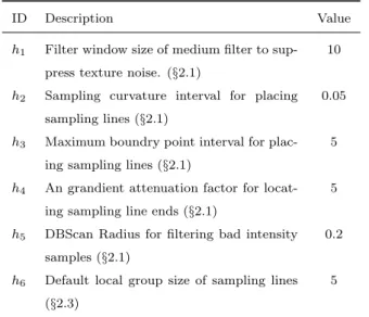
ID Description Value

h1 Filter window size of medium filter to

sup-press texture noise. (§2.1)

10

h2 Sampling curvature interval for placing

sampling lines (§2.1)

0.05

h3 Maximum boundry point interval for

plac-ing samplplac-ing lines (§2.1)

5

h4 An grandient attenuation factor for

locat-ing sampllocat-ing line ends (§2.1)

5

h5 DBScan Radius for filtering bad intensity

samples (§2.1)

0.2

h6 Default local group size of sampling lines

(§2.3)

5

Table 1: Important parameters and their default values

algorithm is then evaluated versus other state-of-the-art 385

shadow removal methods using both visual comparisons and our improved quantitative evaluation measurements. This includes an additional algorithm for ground truth rec-tification on the current state-of-the-art open dataset [1].

3.1. Variability under Different User Inputs

390

(a) single stroke test 1 (b) single stroke test 2

(c) result with 1 stroke (d) result with more strokes Figure 8: Variable input behaviours: The top row shows two ex-amples using single input strokes. We supply 10 exex-amples of single strokes placed in different locations and used as input (shown in dif-ferent colours). The 2 grey-level images show the visualised probabil-ity of each pixel being marked in these 10 independent tests. Fewer grey pixels indicate higher stability,i.e.the image should only show black (0% probability) and white (100% probability) pixels when it is absolute stable. The bottom row shows examples highlighting how additional strokes can improve the detection result (binary mask).

Given user-specified single strokes, our shadow detec-tion generates stable results in different condidetec-tions (e.g. Fig. 8 (a) and Fig. 8 (b)). When the shaded surfaces are made of different materials and a single stroke cannot cover all of them, multiple strokes may be needed. Often, more 395

strokes can lead to more robust detection result (e.g.Fig. 8

(c) and Fig. 8 (d)).

3.2. Rectification of Ground Truth

In the dataset of Guo [1], many of the shadow-free ground truth images are collected by entirely blocking the 400

natural light in the scene. This unfortunately causes in-consistency in the brightness between some shadow-test images (e.g. Fig. 9 (a)) and corresponding shadow-free ground truth (e.g. Fig. 9 (b)). This will result in un-faithful quantitative evaluations in some test cases. To 405

compensate for this, ground truth images of this kind can be globally re-lit (e.g. Fig. 9 (c)) before evaluation. The RGB scale vector for global relighting can be estimated from the average RGB intensity of the common lit area. Lit pixels are first detected using a ratio imageIgr=IIgt

410

whereIis the original shadow image,Igtis the shadow-free

ground truth,is an operator for element-wise division. K-Means clustering [20] is then used to divide the ratios into two clusters and the cluster with higher average ratios are identified as the lit cluster.

(a) Shadow Image (b) Original GT (c) Rectified GT

Figure 9: Ground truth adjustment: An example rectified shadow-free ground truth image (c) obtained by correcting (b) shows a higher consistency with the test image (a). Note that in the original ground truth, the corrected image shows dark pixels as opposed to expected light ones (corrected in our rectified example).

415

3.3. Quantitative Evaluation

In previous work [1], the quality of shadow removal is measured by the per-pixel Root-Mean-Square-Error (RMSE) between the shadow removal result and shadow-free ground truth in RGB colour space. However, the size and darkness 420

of a shadow are often variable and this can result in biased shadow removal quality measurements. For example, an unprocessed image with a small area of shadow can have a smaller RMSE than the error of an image which has a

large area of shadow that has only been partially corrected. 425

Therefore, images with larger or darker shadows can affect the overall score. Our error ratio is therefore computed as

Er=En/Eo whereEnis the RMSE between the shadow-free ground truth and shadow removal result, andEois the RMSE between the shadow-free ground truth and the orig-430

inal shadow image. All error measurements are assessed in RGB colour space. This normalised measure reflects the degree of shadow removal towards the ground truth inde-pendent of original shadow intensity and size. To assess the robustness, the standard derivation is also computed 435

for each measurement.

Extending previous work on ground truth based evalu-ation [1], we categorise shadows into different types. In our test, additional scores for particular categories of shadows with soft penumbra and strong texture background are 440

shown. These special categories are included because they are generally more difficult to process compared with low texture backgrounds with compact shadows. Quantitative results are presented in Tab. 2, wherestarred columns refer to pixels just in the shadow region being considered, and 445

non-starredcolumns refer to the entire image. Our method outperforms the other approaches compared against for most of the scores (especially for soft shadow tests). There are a small number of our scores that are numerically close to the second best ones. However, small numerical differ-450

ences may indicate visually significant artefacts which are shown in the visual comparison sub-section (§3.4).

3.4. Visual Comparisons

Typical examples of our shadow removal algorithm are shown for visual comparison in Fig. 10. Overall, our method 455

produces more qualitatively pleasing removal results against the evaluated methods specially for shadow boundary re-covery. However, minor artefacts are sometimes noticeable when the input image has a highly irregular soft penumbra, or the background of the shadow area is highly shadow-460

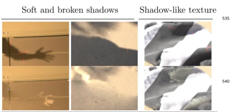
like. Fig. 11 shows some difficult cases where shadows

are soft and broken or cast on a shadow-like background. These typical examples of limitation cases identified in all tested shadow removal methods represent future research challenges in our field.

465

4. Conclusion

A user-friendly shadow removal method has been psented that provides several innovations in this area of re-search. This includes simple user input, intelligent inten-sity sampling, a local group processing based shadow scale 470

estimation and robust colour correction. The presented al-gorithm has been quantitatively evaluated using the stan-dard dataset in this area, and demonstrates state-of-the-art performance. Visual comparisons are also presented for a large number of shadow removal cases taken from 475

the evaluation data set. Through our analysis, difficult shadow removal cases such as broken and soft shadows, and shadows on strong texture background have also been identified. These represent exciting research challenges in our area.

480

Acknowledgement

This work was supported by Engineering and Physi-cal Sciences Research Council (EPSRC) (EP/M023281/1, EP/M001768/1).

References

485

[1] R. Guo, Q. Dai, D. Hoiem, Paired regions for shadow detection and removal, Transaction on Pattern Analysis and Machine In-telligence PP (99) (2012) 1–1.

[2] E. Arbel, H. Hel-Or, Shadow removal using intensity surfaces and texture anchor points, Transaction Pattern Analysis and

490

Machine Intelligence 33 (6) (2011) 1202–1216.

[3] G. D. Finlayson, M. S. Drew, C. Lu, Entropy minimization for shadow removal, International Journal on Computer Vision 85 (1) (2009) 35–57.

[4] Q. Yang, K.-H. Tan, N. Ahuja, Shadow removal using bilateral

495

filtering, Transaction on Image Processing 21 (10) (2012) 4361– 4368.

Guoet al.[1] Suet al.[11] Zhanget al.[19] Gonget al.[18] Ours E E* E E* E E* E E* E E* Softness 0.79 (0.41) 0.63 (0.38) 0.63 (0.31) 0.69 (0.67) 0.53 (0.28) 0.33 (0.25) 0.61 (0.27) 0.44 (0.27) 0.49 (0.27) 0.32 (0.27) Textureness 0.72 (0.41) 0.46 (0.36) 0.77 (0.35) 0.61 (0.42) 0.65 (0.29) 0.45 (0.59) 0.62 (0.26) 0.42 (0.25) 0.63 (0.28) 0.39 (0.23) Overall 0.67 (0.35) 0.48 (0.36) 0.78 (0.43) 0.97 (1.14) 0.67 (0.37) 0.46 (0.51) 0.60 (0.26) 0.42 (0.33) 0.59 (0.28) 0.40 (0.31)

Table 2: Categorised quantitative test results. The non-stared and stared columns indicate the error score where all pixels in the image are used, and just shadow area pixels respectively. The categories of “Soft” and “Texture” refer to shadow images with soft penumbra and strong texture background respectively. “Overall” is the average result for all test cases in the data set. Method [1] is trained using a large shadow detection data set from [12]. The standard derivation for each measurement are in brackets.

Original Guo [1] Su [11] Zhang [19] Gong [18] Ours Ground Truth

Figure 10: Comparisons of our method against existing state-of-the-art techniques using ground truth images from [1]. Please magnify to examine penumbra recovery in detail. The first column images are the original shadow images with our user input strokes marked in red.

Soft and broken shadows Shadow-like texture

Figure 11: Universal failure cases – where all the leading methods create highly visible image artefacts and fail to remove the shadow. [5] C. J. J. Yoon, T.J.Ellis, Shadowflash: an approach for shadow removal in an active illumination environment, in: British Ma-chine Vision Conference, BMVA, 2002.

500

[6] M. Drew, C. Lu, G. Finlayson, Removing shadows using flash/noflash image edges, in: International Conference on Mul-timedia and Expo, IEEE, 2006, pp. 257–260.

[7] N. Salamati, A. Germain, S. Susstrunk, Removing shadows from images using color and near-infrared, in: International

Confer-505

ence on Image Processing, IEEE, 2011, pp. 1713 –1716. [8] G. Finlayson, C. Fredembach, M. Drew, Detecting illumination

in images, in: International Conference on Computer Vision, IEEE, 2007, pp. 1–8.

[9] T.-P. Wu, C.-K. Tang, M. S. Brown, H.-Y. Shum, Natural

510

shadow matting, Transactions on Graphics 26 (2) (2007) 8. [10] F. Liu, M. Gleicher, Texture-consistent shadow removal, in:

Eu-ropean Conference on Computer Vision, Springer, 2008, pp. 437–450.

[11] Y.-F. Su, H. H. Chen, A three-stage approach to shadow field

515

estimation from partial boundary information, Transaction on Image Processing 19 (10) (2010) 2749–2760.

[12] J. Zhu, K. G. G. Samuel, S. Masood, M. F. Tappen, Learning to recognize shadows in monochromatic natural images, in: Inter-national Conference on Computer Vision and Pattern Analysis,

520

IEEE, 2010, pp. 223–230.

[13] J.-F. Lalonde, A. A. Efros, S. G. Narasimhan, Detecting ground shadows in outdoor consumer photographs, in: European Con-ference on Computer Vision, 2010, pp. 322–335.

[14] J.-B. Huang, C.-S. Chen, Moving cast shadow detection using

525

physics-based features, in: International Conference on Com-puter Vision and Pattern Analysis, IEEE, 2009, pp. 2310 –2317. [15] J. Yao, Z. M. Zhang, Hierarchical shadow detection for color aerial images, Computer Vision and Image Understanding 102 (1) (2006) 60–69.

530

[16] E. Salvador, A. Cavallaro, T. Ebrahimi, Cast shadow segmenta-tion using invariant color features, Computer vision and image understanding 95 (2) (2004) 238–259.

[17] Y. Shor, D. Lischinski, The shadow meets the mask: Pyramid-based shadow removal, Computer Graphics Forum 27 (2) (2008)

535

577–586.

[18] H. Gong, D. Cosker, Interactive shadow removal and ground truth for variable scene categories, in: Proceedings of the British Machine Vision Conference, BMVA Press, 2014.

[19] L. Zhang, Q. Zhang, C. Xiao, Shadow remover: Image shadow

540

removal based on illumination recovering optimization, Trans-actions on Image Processing 24 (11) (2015) 4623–4636. [20] G. A. Seber, Multivariate observations, Vol. 252, John Wiley &

Sons, 2009.

[21] J. H. Friedman, J. L. Bentley, R. A. Finkel, An algorithm for

545

finding best matches in logarithmic expected time, ACM Trans-actions on Mathematical Software 3 (3) (1977) 209–226. [22] E. Cliffs, Two-Dimensional Signal and Image Processing,

Pren-tice Hall, 1990.

[23] S. Martucci, et al., Image resizing in the discrete cosine

trans-550

form domain, in: Image Processing, 1995. Proceedings., Inter-national Conference on, Vol. 2, IEEE, 1995, pp. 244–247. [24] M. Ester, H.-P. Kriegel, J. Sander, X. Xu, A density-based

al-gorithm for discovering clusters in large spatial databases with noise., in: SIGKDD Conference on Knowledge Discovery and

555

Data Mining, Vol. 96, ACM, 1996, pp. 226–231.

[25] S. Paris, F. Durand, A fast approximation of the bilateral fil-ter using a signal processing approach, Infil-ternational Journal of Computer Vision 81 (1) (2009) 24–52.

[26] J. Nocedal, S. Wright, Numerical optimization, 2nd Edition,

560

Springer series in operations research, Springer, 2006, Ch. 18. [27] D. Garcia, Robust smoothing of gridded data in one and higher

dimensions with missing values, Computational Statistics & Data Analysis 54 (4) (2010) 1167–1178.

[28] M. Bertalmio, G. Sapiro, V. Caselles, C. Ballester, Image

in-565

painting, in: Transaction on Graphics, ACM, 2000, pp. 417– 424.

[29] E. Reinhard, M. Ashikhmin, B. Gooch, P. Shirley, Color trans-fer between images, IEEE Computer graphics and applications 21 (5) (2001) 34–41.