Consistency on the Vertices, Edges and Mask: A Semi-Supervised Learning Approach for Image Segmentation

(1)

Final Bachelor’s Thesis

Consistency on the Vertices, Edges and

Mask: A Semi-Supervised Learning

Approach for Image Segmentation

Degree in Mathematics & Degree in Engineering Physics

Author:

Jordi

_{Fortuny Profit´}

_os

Supervisor:

Sanja

_Fidler

Local Tutor:

Xavier

_Gir´

_{o i Nieto}

(2)

Jordi Fortuny Profit´os: Consistency on the Vertices, Edges and Mask: A Semi-Supervised Learning Approach for Image Segmentation© May 2019

A Bachelor’s Final Thesis Submitted to the Escola Tècnica d’Enginyeria de Telecomunicació de Barcelona (ETSETB), Facultat de Matemàtiques i Estad´ıstica (FME) and Centre de For-mació Interdisciplinària Superior (CFIS) of the Universitat Politècnica de Catalunya (UPC) in partial fulfilment of the requirements for the degrees of doble titulació en el grau de matemàtiques i grau d’enginyeria f´ısica.

Thesis done at the Vector Institute, University of Toronto, under the supervision of Prof. Sanja Fidler.

supervisor:

Sanja Fidler

home supervisor:

Xavier Gir´o i Nieto

location:

(3)

Computer Science is no more about computers than astronomy is about telescopes. — Edsger Dijkstra

(4)

(5)

Abstract

In this thesis, we present a novel method for performing image

segmenta-tion in a semi-supervised approach, which we consider to be particularly

relevant because of the substantial cost of obtaining pixel-wise annotations

required to train supervised. This method, that we will call Consistency

on the Vertices, Edges and Mask, is one of the first methods that can be

used for training deep neural networks to perform image segmentation in

a semi-supervised setting where only a small portion of training data is

labeled. In our setting, we train a network to predict masks, edges and

vertices for a given input image, and then we penalize the network for not

being consistent with its predictions obtaining the theoretical edges an

vertices from the predicted mask using a derivable version of the Canny

edge detector. We also present results on the Cityscapes Dataset where

we obtain outstanding results achieving about 92% of the fully supervised

performance labeling only 10% of the data and 98% labeling 25%.

This thesis also contains a brief introduction on the field of deep

learn-ing and semi-supervised learnlearn-ing, relevant previous work that has been

published in the last year which inspired this work and finally,

informa-tion on the architecture of our model and its performance as well as some

experiments, results and ablation studies.

KeyWords:

Computer Vision

· Machine Learning

· Deep Learning

· Semi-Supervised Learning

· Image Segmentation

· Cityscapes Dataset

· Consis-tency

· Canny Edge Detector.

(6)

(7)

Acknowledgments

I would like to express my very great appreciation to Professor Sanja Fidler,

my research supervisor, for all her valuable and constructive suggestions

during the planning and development of this research work. I would also

like to thank Dr. David Acuna and Kevin Shen, for their advice and

assis-tance in keeping my progress on schedule. Their willingness to give their

time so generously has been very much appreciated.

I would also like to thank the staff of the Vector Institute for enabling

me to use their offices and their computing resources, allowing me to

par-ticipate in talks, events and learning sessions as well as assisting me for

any trouble inside or outside the office.

I also wish to thank various people for their indirect contribution to this

project, Prof. Miguel ´

Angel Barja, Prof. Toni Pascual, Prof. Xavier Gir´

o

and Prof. Eduardo Alarc´

on, allowing me the opportunity to spend time

conducting research at the Vector Institute under one of the excellence

mobility CFIS grants.

I would like to thank all the colleagues that I’ve worked with during my

research internship, specially Eric Guisado, Rafel Palliser and D´ıdac Sur´ıs,

with whom I have shared moments of deep anxiety but also of big

excite-ment. Their presence was very important in a process that sometimes can

be felt as tremendously solitaire.

I would also like to extend my thanks to my life partner, Ariadna,

with-out whom it would have been impossible to carry on this project. She has

been the light of my life for the last two years and she has given me the

strength and motivation to get things done. This paper is dedicated to her.

Finally, I wish to thank my parents for their support and encouragement

throughout my study.

(8)

(9)

List of Figures

2.1 Example of a convolution . . . 19

2.2 Example of a fully connected layer . . . 20

2.3 Block of a residual learning architecture . . . 21

2.4 Comparison between deep architectures . . . 22

3.1 Pi Model and Temporal Ensembling Model . . . 26

3.2 Pi Model Pseudocode Algorithm . . . 27

3.3 Temporal Ensembling Pseudocode Algorithm . . . 27

3.4 Polygon-RNN annotation tool . . . 28

3.5 Polygon-RNN++ annotation tool . . . 28

3.6 Polygon RNN architechture . . . 29

3.8 Evaluation Network of Polygon-RNN++ . . . 30

3.7 Polygon-RNN++ ResNet . . . 31

3.9 Polygon-RNN++ architechture . . . 31

4.2 Example image of the Cityscapes dataset . . . 34

4.1 Map of the cities of the Cityscapes dataset . . . 34

4.3 Example image of the Cityscapes dataset . . . 35

4.4 Example output of some masks using Deeplabv3+ . . . 36

4.5 Example input image from the Cityscapes Dataset . . . 37

4.6 Examples of the Ground Truth Data of the Cityscapes Dataset . . . 38

4.7 Skip-Connection ResNet-50 backbone . . . 42

5.1 IoU when different data regimes are labeled . . . 45

5.2 F-score with threshold of 1 pixel when different data regimes are labeled . . . 46

5.3 F-score with threshold of 2 pixels when different data regimes are labeled . . . . 46

5.4 Visual Results . . . 49

5.5 Visual Results . . . 50

(11)

List of Tables

4.1 Cityscapes Dataset Splitting . . . 34 4.2 Cityscapes Pixel Segamentation Benchmark . . . 36 5.1 Best trained models on different data regimes . . . 47 5.2 Ablation Study on the Intersection over Union (IoU) and the F-score with

threshold of both 1 and 2 pixels using 10000 labels. . . 47 5.3 Ablation Study on the Intersection over Union (IoU) and the F-score with

threshold of both 1 and 2 pixels using 4000 labels. . . 48

(12)

(13)

1.

Introduction

1.1 Motivation

Inside the field of computer science, there is a research area that lacks of a precise definition but curiously, that is what has it one of the most promising fields of study in the recent years. Researchers and developers of Artificial Intelligence (AI) are guided by a rough sense of direc-tion and an imperative to “get on with it.” However, on 2010 Nils J. Nilsson [20] provided a useful definition that is still used nowadays: ”Artificial intelligence is that activity devoted to making machines intelligent, and intelligence is that quality that enables an entity to function appropriately and with foresight in its environment.”

In fact, sometimes the field of AI is called machine intelligence since its goal can be understood as creating ”intelligent agents” that can perceive their environment and take actions in order to achieve specific goals and tasks through flexible adaptation. Pamela McCorduck [18] explains that AI suffers from a repeating pattern, the “AI effect” —AI brings a new technology into the common fold, people become accustomed to this technology, it stops being considered AI, and newer technology emerges. Nevertheless, all that technology is always focused on mimicking cognitive functions that are associated with human minds, such as pattern recognition, learning, image classification, problem solving...

One of the newest areas inside Artificial Intelligence is Deep Learning (DL) which at the same time is also part of Machine Learning. DL is the field that learns data representations through basically deep neural networks and recurrent neural networks. Deep learning can be used in a lot of different computer science environments, but it is typically associated with image recognition and computer vision (although one can find examples in the literature [3] where has been used for medical image analysis, natural language processing, speech recognition, machine translation, drug design and board game programs such as chess or go, where they have produced results superior to human experts and any other ”non-intelligent” existing machine). I personally think that AI is where every computer scientist knows that they can find the solution they need or where they should research for developing that solution, and hence has awaken interest of mathematicians, engineers and even physicists or doctors. As a mathematician, I love the statistics of the models, how you can translate what you code to mathematical models and the ”good praxis” to first formulate how the maths of the model are gonna behave. On the other hand, as an engineer, I love developing the models and fight to solve all the problems that the coding part of the project proposes.

(14)

14 CHAPTER 1. INTRODUCTION This thesis contains a summary of all the research and work conducted under the supervision of Prof. Sanja Fidler during my internship at the Vector Institute in Toronto. The main focus of the work has been Semi-Supervised Deep Learning and the following chapters contain a brief introduction of the field to the reader, some of the relevant related work that has been done in the previous years as well as my personal contribution to the field with results and my personal thoughts and conclusions about the internship.

1.2 Objectives

In the field of computer science, and more concretely in the field of deep learning, one of the objectives of the researchers worldwide is to extract as many information as possible from a given dataset. This objective can also be thought as understanding how big should the datasets be, or how many data points should be labeled in order to obtain good performance. In a field where bigger is not necessarily better due to the acquiring, storage and labelling costs, it is essential to solve this questions

A lot of research has been conducted in the previous years towards the goal of reducing the dataset size [21], choosing more accurately what images should be labeled [26] or even how a smaller network can distill all the information of a big dataset [31]. There is also a branch of research that focuses on how is it possible to complement a labeled dataset with non-labeled images that are from the same domain. This is Semi-Supervised Learning and the recent literature has proven it can be really useful on image classification [16, 22, 29].

The goal of this thesis and the objective of my internship were finding a way to use unlabeled data to improve the performance on image segmentation (i.e. presenting Semi-Supervised Learning for image segmentation). I consider this to be a very relevant topic nowadays since we are living in the big data era where large companies are hunting out there for billions and billions of data. It would be really nice for all those companies, but also for research purposes, to be able to achieve the same performance with only 10% of the available data. First step was being able to obtain impressive results in image classification and the next natural step would be learning how to segment semi-supervising.

In order to achieve this big objective, other intermediate goals have arisen such as under-standing the current state-of-the art results, underunder-standing the recent literature and learning the programming skills needed. In fact, at the beginning of this internship, my supervisor advised me to read a lot and she assigned me tasks such as coding in Pytorch [23] (which to my understanding is the best library in python for Deep Learning) or summarizing some of the most recent techniques from relevant papers which form a future point of view it is something that I am completely grateful to have done.

Another important goal that was set at the begging of this internship was being able to come back to Barcelona with more knowledge than when I left. Learning has always been one of my passions and I feel specially happy with the opportunities that this project has given me for doing such thing. For being a researcher at the Vector Institute, I’ve been able to assist to at least 10 research talks, 4 round-tables, 4 group meeting with the supervisor’s team, a dozen student discussion meetings, a Fields Institute talk and Vector’s insight meetings on a monthly basis, and hence improving as a scientist and as a person.

(15)

1.2. OBJECTIVES 15 Finally, the last objective that I considered was growing as a human being. It is a goal that I have always had in mind since I have conscience of my decisions and I think it is really important to make an effort to understand people with different backgrounds, religions and cultures from the ones we are used in our country. I think that visiting Toronto, the most multicultural city in the world, and the Vector Institute were some of the best researchers worldwide spend 10 hours on a daily basis, has allowed me to learn a lot, understand different points of view and maintain a lot of interesting conversations.

(16)

(17)

2.

Deep Learning and Semi-Supervised

Learning

On May 2015, Nature published a short review titled ”Deep Learning” [3]. On the abstract, LeCun, Bengio and Hinton summarized how deep learning methods improved at that time the state-of-the-art in speech recognition, visual object recognition, object detection and many other domains such as drug discovery and genomics. Moreover, they highlight the multiple levels of abstraction that such methods ”learn” using the back-propagation algorithm to update its internal parameters.

A quick search into any search engine would lead one to some definitions explaining that DL is a function that imitates the workings of the human brain trying to process data and create patterns to make the right decisions, or that DL is a subset of machine learning and AI that consists in building networks capable of learning from data that is unstructured or unlabeled, or even one can find a magnification of the field as stated by Andrew Ng in its own web-page www.deeplearning.ai: ”Deep Learning is a superpower. With it you can make a computer see, synthesize novel art, translate languages, render a medical diagnosis, or build pieces of a car that can drive itself. If that isn’t a superpower, I don’t know what is.”

But, what are the pieces that build together that concept? What are the basics that one must know to understand DL? I would say that there are two main networks that are used in the 95% of Deep Learning Applications, Convolutional Neural Networks and Recurrent Neural Networks. Each one has its own particularities and ingredients, and while the first is mainly used for of those visual object recognition and object detection, the later is more effective for visual question answering or machine translation. On this paper the focus lies on the first one because recurrent neural networks are not used in this project.

Semi-supervised Learning is a class of Machine Learning and Deep Learning that uses both labeled data and unlabeled data. In that sense, it is able to train both using supervision of the tasks through the labeled data where ground truth is available and unsupervised on the unlabeled data (i.e. it is able to use the unlabeled data to train and improve although it doesn’t has labels to understand it).

This section explains the basics of the methods used in the literature to provide context and knowledge to the reader about the different networks, structures and techniques used in the project. It first focus on Deep Learning and shows and example of one very important network used in this project and there is also presented a brief introduction to semi supervised learning.

(18)

18 CHAPTER 2. DEEP LEARNING AND SEMI-SUPERVISED LEARNING

2.1 Deep Learning

Deep Learning is such an extensive field that one could write an entire book about it, and I would like to address to the reader with some of my suggestions of really good deep learning books that they could find in the bibliography: [8, 11, 25]. Specially, I would recommend ”Deep Learning for Computer Vision with Python” [25], the book that Adrian Rosebrock, phD and entrepreneur published a couple of years ago. It has received lots of good reviews from other successful authors such as Francois Chollet, AI researcher at Google and creator of Keras, a python library, that said:

This book is a great, in-depth dive into practical deep learning for computer vision. I found it to be an approachable and enjoyable read: explanations are clear and highly detailed. You’ll find many practical tips and recommendations that are rarely included in other books or in university courses. I highly recommend it, both to practitioners and beginners. — Francois Chollet

I personally think that this book is useful to understand the basics of deep learning and also the techniques that are used in object detection and segmentation while at the same time it provides contrasted theory and Python implementation.

Having said that, in this section I would like to explain some of the basics of deep learning that are most used in this project. I refer the reader to the bibliography to extend their knowledge in Deep Learning.

2.1.1 Neural Networks

Artificial neural networks (ANN) are machine learning frameworks that were inspired by the biological neural networks that constitute animal brains [30]. The goal of this frameworks is being able to ”learn” to process complex data inputs and perform tasks without any given a priory rule, just only considering the examples given during training, as a human being would do. An ANN [2] is formed by a collection of connected units or nodes called artificial neurons because they model model the neurons in a biological brain. The neurons are connected like the synapses in a biological brain and can transmit a signal from one to another. In common ANN implementations, all the input signals are real numbers and every neuron outputs another real number obtained by computing a non-linear function of the sum of all the inputs averaged by some weights and bias. Those weights and bias are the learnable parameters of the ANN and an optimization problem will be solved in order to obtain a local minima (or global ideally) according to some loss function that could generalize to any input.

Normally, the neurons are aggregated into layers and the synapse function may vary from one layer to another. In an ANN, the signals travel from the first (or input) layer until the last (or output) layer through all different neuron layers and at the end, a loss function is computed. Normally this loss function will be differentiable with respect to the network weights and then all those parameters are optimized via a backpropagation algorithm.

2.1.2 Convolutional Neural Networks

Convolutional Neural Networks (CNNs) are Neural Networks that are made up of neuron layers that have convolutional kernels with learnable weights and biases. Each of the neurons receives one or some inputs and performs some operations that can be expressed as dot products

(19)

2.1. DEEP LEARNING 19

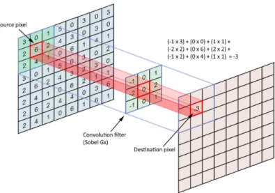
Figure 2.1: Example of a convolution with a convolutional filter of dimensions (3,3,1) and a input tensor of size (8,8,1).

and additions and then usually there is a non-linearity. This operations make the network differentiable with respect to its weights. In the following, there is presented a list of the 5 layers that are present in every architecture of a CNN, with the operations and details that are used.

• Inputlayer: The input layer is just the first input that recieves the model. It typically is an image which would have size (h, w,3) whereh andw are the number of heigh and width pixels of the image and 3 represent the RGB channels. In Deep Learning, it is very typical to work with batches of data, so the input layer will be a tensor (b, h, w,3) whereb just indicates how many images fit in the memory of the GPU and are processed at the same time by the computer.

• Convolutional layers: This layers are the ones that give the name to the entire network and it is not in vain because since their discovery, when the input is and image they are always present. Let’s consider that the input of one of those layers is a tensor of size (h, w, cin). Then this layers have cout kernels of size (hk, wk, cin) of learnable weights that

will be convolving on top of the input tensor (i.e. computing a local dot product) to produce an output of size (hout, wout, cout) where hout and wout are determined by the

padding and the stride factors. Figure 2.1 shows how the dot product in a convolution layer are performed. Padding (or more typically zero-padding) is a factor that determines how many extra rows and columns one will add on the sides of the image. It is a common strategy to preserve size. On the other side, to downsample the spatial dimensionsh and w one could use convolutional layers with stride. The stride factor indicates how many pixels the filter is moving at a time. For a 3x3 convolution as in figure 2.1, the standard stride factor is 1 and the padding factor is also 1 resulting an output with the same spatial dimension as the input.

• Pooling layers: The pooling layers perform a downsampling operation along the spatial dimensions: width and height. In order to do so, the pooling operation converts regions of the image of squared size (typically 2 x 2) into one value, hence reducing the spatial dimensions by 2 each (or the volueme by 4). There are basically two different types of pooling: Average pooling and max pooling. The first one returns the average of the neighbours while the later just returns the maximum of them.

• Fully Connected layers: This layers connect all the input neurons to all the output neurons. They are typically used as last layers in a classification problem because they

(20)

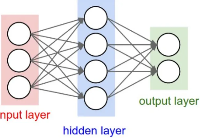
20 CHAPTER 2. DEEP LEARNING AND SEMI-SUPERVISED LEARNING can connect through weights and bias all the input features into output probabilities of each class. Figure 2.2 shows an example of two fully connected layers in a configuration with 3 neurons in the input layer, 4 in the hidden layer and 2 classes as the output.

Figure 2.2: Example of a toy neural network with two fully connected layers.

• Non-linearlayers: Non linear layers or also typically called Rectifier Linear Units (ReLU, Leaky ReLU) are layers that preserve the spatial dimensions and are defined as the positive part of its argument with maybe some alteration:

ReLU(x) =x+=max(0, x) LeakyReLU(x) =    x+=max(0, x), ifx >0 −α·x, ifx <0 where usuallyα= 0.01

An example of how one could use a CCN to classify images according to their content would be the following [17]:

Consider images from the CIFAR-10 dataset [15], those images have shape (32,32,3) pixels and contain images within 10 different classes: cat, dog, bird, horse, frog, deer, automobile, train, ship and airplane.

1. Theinput layer will be a batch of size (b,32,32,3)

2. The first layer we could use is64 3x3 convolutionalfilters with one pixel of zero-padding and stride 1.

3. Then the resulting dimensions will be (b,32,32,64) and after applying a ReLUlayer and a2x2 MaxPooling we will obtain a tensor of dimensions (b,16,16,64) with all positive values.

4. Next, use again64 3x3 convolutional filters with one pixel of zero-padding and stride 1 followed by a ReLU layer and a 2x2 MaxPooling. This results into a tensor of dimensions (b,8,8,64)

5. Follow up with 128 3x3 convolutional filters with stride 2 resulting into a (b,4,4,128) tensor.

6. Finally, end with aLeaky ReLU, another2x2 MaxPooling with α= 0.01 and afully connected layer to compute the class scores, resulting in volume of size (b,1x1x10), where each of the 10 numbers correspond to a class score, such as among the 10 categories of CIFAR-10.

(21)

2.2. RESNET 21 As with ordinary Neural Networks and as the name implies, each neuron in the fully connected layer will be connected to all the numbers in the previous volume, so in order to reduce dimensionality of the parameter space, it is important to use the convolutional filters combined with the poolings. As part of my deep learning training, I designed this network and it obtained around a 85% accuracy on the CIFAR-10 dataset [15]. Code can be found on Appendix 1.

2.2 ResNet

As deep learning architectures go deeper with convolutional layers, they are more difficult to train because the number of parameters is bigger and more importantly because backpropagation has to travel through more layers. On 2015, Microsoft’s Deep Learning researchers He, Zhang, Ren and Sun [13] presented on the conference about Computer Vision and Pattern Recognition (CVPR) a model that has a deep architecture but was more easy to train than before: ResNet.

Figure 2.3: Representation of a building block of a residual learning architecture. Figure originally published in [13].

ResNet is the abbreviation of Residual Net-work and this name was given because the solution of the above mentioned problem lies in building a new architecture with residual blocks (see Figure 2.3). Each block consists on two weight convolutional layers as well as batch normalization and a non linearity (such as ReLU or leaky ReLU) that are applied to an inputxand then added to the same inputx before going into the next block. In that sense, the network is not predicting how to change the input to match the desired output but only the residual transformations that should be applied to the input to make a better version of it.

On figure 2.4 one can see schematically the difference between some of the architectures that were used as a baseline in [13] (left and middle) as well as a 34-layer ResNet (right). One can see that the main change is the fact that there are residual connections every two layers in the residual network (i.e. it is build with residual building blocks). Note that when a connection is represented with a dotted line means that there has been a down-sampling operation applied to the input data.

That trick, which is relatively easy to understand, broke all the state-of-the-art performances on image classification and object location and ResNet is still one of the most used architectures in deep learning. Particularly, in this project, the backbone architecture is a pretrained ResNet which is used to obtain reliable features of the input images.

2.3 Semi Supervised Learning

When working under a semi-supervised regime it is typical to assume at least one of the following [6]:

• Continuity: Data points which are close in the feature space, are more likely to share a label. This assumption is also assumed in almost all supervised vision problems when the objective is to find a good feature space representation through which the decision boundaries should be easy to find.

(22)

22 CHAPTER 2. DEEP LEARNING AND SEMI-SUPERVISED LEARNING

Figure 2.4: Comparison between deep architectures. Left: VGG [27], the deep model presented by Google,Middle: A deep architecture with 34 layers,Left: A deep residual architecture of also 34 layers. One can see how the residual one is completely build through residual building blocks. Figure originally published in [13].

(23)

2.3. SEMI SUPERVISED LEARNING 23 • Data Clustering: The data points are grouped into discrete clusters, and points in the same cluster are more likely to share a label. This doesn’t necessarily mean that there are as many clusters than labels, it can be more clusters than labels, meaning that more than one cluster will have the same label (distributed labelling) or even more labels than clusters, meaning that some clusters will have data from different labels (close labelling). • Manifold approximation: The data points can be approximately found on a manifold of much lower dimension than the input space. Then the objective will be to learn the manifold and work on the manifold space where less parameters are needed.

As one can see, all those assumptions make it easy to exploit the use of unlabeled data. In the first scenario, one will penalize if the model predicts different labels for nearer points, on the second one, the penalization would be imposed within clusters and the last scenario allows to penalize the model if it represents the data in many dimensions.

In image classification, the continuity and clustering assumptions are the most used in the recent literature [16, 22, 29]. More emphasis on this point will be made in the section 3 where there are presented some papers that are state-of-the-art on Semi Supervised image classification and that have been used as an inspiration of the project.

(24)

(25)

3.

Related Work

This chapter contains an introduction to some of the related work and papers that have inspired this project. The goal of this chapter is to familiarize the reader with the notation and concepts that are used in the semi-supervised learning framework as well as present the papers that improved my knowledge and motivated all my ideas.

3.1 Related Work in Semi Supervised Learning

In the following, there are presented some approaches of classical semi supervised learning proposed in [16] and [29] described in the context of traditional image classification networks: Let D be the training data consisting of N inputs, M of which are labeled. Let xi where

i∈ {1...N}be the inputs and let the set Lcontain the labels yi wherei∈L. For every iin L

there is a correct label yi∈ {1...C} where C is the number of classes. Letωt be weighting ramp

factor that scales from 0 towmax.

These two papers have served as inspiration for the consistency technique used in our semi-supervised approach. Personally, I find them surprisingly interesting and simple at the same time and I think that is precisely this simplicity that makes them relevant. A simple technique that thinking a bit out of the box can be used in another setting under different conditions.

The first paper [16] presents a simple and efficient method for training deep neural networks in a semi-supervised setting. They introduce self-ensembling, where they form a consensus prediction (i.e. averaging label predictions) of the unknown labels using the outputs of the network-in-training on different epochs and under different regularization and input augmen-tation conditions. This ensemble prediction can be expected to be a better predictor for the unknown labels than the output of the network at the most recent training epoch, and can thus be used as a target for training. Using our method, they set new records for some standard semi-supervised learning benchmarks and they demonstrate good tolerance to incorrect labels. On the other hand, on the Mean Teacher model [29], the authors suggest that the Temporal Ensembling [16] method fails for large datsets and they propose a method that overcomes this situation. Mean Teacher is a method that averages model weights instead of label predictions. As an additional benefit, Mean Teacher improves test accuracy and enables training with fewer labels than Temporal Ensembling. Without changing the network architecture, Mean Teacher achieves better results than Temporal Ensembling on all the benchmarks.

3.1.1 Π-model

The Π-model relies on evaluating twice the inputs xi through an stochastic network, (i.e.

containing Dropout or applying data augmentation twice) resulting in two different predictions zi and zei. In training mode there are two different loss terms. The first one is the typical cross-entropy loss which can only be evaluated for the labeled data. On the other hand, the

(26)

26 CHAPTER 3. RELATED WORK second component is computed taking the mean square difference between the two predictions zi andzei. Then the total loss (Equation 3.1) is the sum of the supervised and the unsupervised terms weighted by ωt. Hence, in the beginning the total loss and the learning gradients are

dominated by the supervised loss component, i.e., the labeled data only and due to a slow ramp-up weighting function the network learns slowly the consistency terms and does not fall into a degenerate solution with no meaning for classification.

L=Lce+ωtLcons =− 1 L X i∈L logzi[yi] + ωt N N X i=1 z_i2−z_ei2 (3.1)

3.1.2 Temporal Ensembling model

The Temporal ensembling model is also a consistency semi-supervised learning approach that instead of evaluating twice the inputs through the network just uses the network once and keeps in memory aggregated predictions of multiple previous network evaluations as an ensemble prediction. It maintains an exponential moving average of label predictions on each training example, and penalizes predictions that are inconsistent with this target. Hence, it speeds up the training and it alleviates the noisy targets that are obtained from the Π-model based on a single evaluation of the network. The formal structure of the model is the following:

Each input xi is evaluated once per epoch, and a predictionzi is obtained that it is used

both for the typical cross entropy loss term and also a consistency loss term betweenzi and the

target vectorsz_ei. In this model, the target vectors are obtained from the ensemble predictionZi.

Equation 3.2 show the loss and the definitions for the ensemble prediction and target vectors used on this approach. Note thatα is a momentum hiperparameter that controls then memory of the ensemble prediction. Figure 1 shows an original scheme published by the authors in [16].

e zt i = Z_it 1−α (3.2a) L=Lce+ωtLcons=− 1 L X i∈L logzi[yi] + ωt N i=N X i=1 z_i2−zet i 2 (3.2b) Z_it+1=αZ_it+ (1−α)zt_i (3.2c)

Figure 3.1: Scheme of the pi model and the temporal ensembling model. Figure originally published in [16].

(27)

3.1. RELATED WORK IN SEMI SUPERVISED LEARNING 27

Figure 3.2: Pseudocode describing the Pi Model. Figure originally published in [16].

Figure 3.3: Pseudocode describing the Temporal Ensembling Model. Figure originally published in [16].

3.1.3 Mean Teacher model

The Mean teacher model [29] proposes averaging model weights instead of averaging predictions as in the temporal ensembling model. Typically, averaging models or model weights produces a more accurate model than using the final weights of one of the trained model alone. The result is a teacher model which is an average of consecutive student models, and hence the name Mean Teacher. On training time, there will be also two loss terms. The softmax output of the student model is compared with the one-hot label using a classification cost such as cross entropy and with the teacher output using a consistency cost such as a squared-difference loss. Let θbe the parameters of the student model andθ0 from the teacher model. Let f be the result of predicting targets with the network. Equation 3.3 presents this semi-supervised approach whereα,λand ωt are defined as before. Also note that f(x, θ) = zi in the previous models. At the end of

training, both models can be used for prediction but the model teacher is more likely to be correct. As in the other models it is also possible to evaluate the same inputs applying different Gaussian noise or data augmentation.

(28)

28 CHAPTER 3. RELATED WORK θ_t0 =αθ0_t₋₁+ (1−α)θt (3.3a) L=Lce+ωtLcons=− X i∈L yilogf(x, θ) + λωt N i=N X i=1 f(x, θ)2−f(x, θ0)2 (3.3b)

3.2 Polygon-RNN

Figure 3.4: Presentation of the Polygon-RNN annotation tool. Figure originally published in [5]

In this section there are presented two papers (”Annotating Object Instances with a Polygon-RNN” and ”Efficient Annotation of Segmenta-tion Datasets with Polygon-RNN++” [1, 5]) that have inspired this work as well as having been the basis of which the code has been inherited. Both papers are fruit of the work of the Vec-tor Institute and during my internship I’ve been able to learn and discuss topics with its au-thors.

Figure 3.5: Presentation of the Polygon-RNN annotation tool. Figure originally published in [1]l

Polygon-RNN and Polygon-RNN++ [1, 5] are inter-active annotation tools to produce polygonal annota-tions of objects interactively using humans-in-the-loop. The main benefit of using a polygon to annotate in-stances (instead of doing it pixel-wise) is that polygons are sparse and more easy to interact with resulting in less annotator corrections and faster performance. With their publications respectively in 2017 and 2018, both Polygon-RNN and Polygon-RNN++ were trained and evaluated on the Cityscapes Dataset [9] and achieved human-level state of the art performance on the seman-tic classes of car, truck and bus.

3.2.1 Polygon-RNN

Polygon-RNN [5] is an annotation tool for labeling object instances with polygons. The system acts assuming that the user provides the bounding box around the object and it predicts a polygon outlining the object using a Recurrent Neural Network. After the prediction it is possible to correct one or some predicted vertices of the polygon.

The architechture of the model strongly relies on a RNN that predicts a vertex at every time step until it closes the polygon. The inputs of the RNN are a CNN representation of the image crop, as well as the vertices predicted one and two time steps ago, plus the first point. By explicitly providing information of the past two points the RNN gets some help to follow a particular orientation of the polygon. On the other hand, the first vertex helps the RNN to decide when to close the polygon.

The architecture can be trained end-to-end which allows the CNN to be fine-tuned to object boundaries, while the RNN learns to follow these boundaries and exploits its recurrent nature to also encode priors on object shapes. Figure 3.6 shows an overview of the model.

(29)

3.2. POLYGON-RNN 29

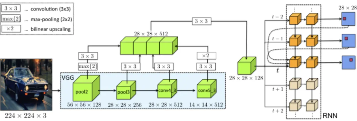
Figure 3.6: Scheme of the architecture of the Polygon-RNN model. At each time step of the RNN-decoder (right), an image representation is fed in using a modified VGG architecture. The RNN is a two-layer convolutional LSTM with skip-connection from one and two time steps ago. At the output at each time step, a new vertex of the polygon is predicted. Figure and description originally published in [5].

More concretely, the RNN is fed by an image representation which is obtained using a modi-fied VGG-16. The modifications are the following: Removal of the fully connected layers as well as the last max-pooling layer, pool5. The output of this modified network has a downsampling factor of 16. On top of that, a couple additional convolutional layers with skipconnections are used to fuse information from the previous layers and upscale the output by factor of 2. This allows the CNN to extract features that contain both low-level information about the edges and corners, as well as semantic information about the object. The latter helps the model to “see” the object, while the former helps it to follow the object’s boundaries.

The Recurrent Neural Network that is used in Polygon-RNN is a Convolutional Long-Short-Term-Memory(LSTM) which operates in 2D and hence it preserves the spatial information received from the CNN. Furthermore, a Convolutional LSTM employs convolutions, thus greatly reducing the number of parameters to be learned compared to using a fully-connected RNN. To recall, in its simplest form, a single layer Convolutional LSTM computes the hidden stateht

given the input xt according to the following equations:

      it ft ot gt       =Wh∗ht−1+Wx+xt+b (3.4) ct=σ(ft)·ct1+σ(it)·tanh(gt) (3.5) ht=σ(ot)·tanh(ct) (3.6)

In this equations: i, f and o denote the input, forget, and output gate while h is the hidden state and c is the cell state. σ denotes the sigmoid function and · indicates an element-wise product and∗ a convolution. The Wh andWx matrices denote the hidden and input kernels

which are 3x3 and have 16 channels. The vertex prediction is formulated as a classification task: at time step t, each vertex is encoded as a one-hot vector of a D×D+1 grid, where the D×D dimensions represent the possible 2D positions of the vertex, and the last dimension corresponds to the end-of-sequence token. The position of the vertices are thus quantized to the resolution of the output grid which was found to be optimum being 28 pixels. Finally the outputs are upsampled to original resolution of the image.

(30)

30 CHAPTER 3. RELATED WORK

3.2.2 Polygon-RNN++

Polygon-RNN++ [1] is a following work of Polygon-RNN [5] that includes several important improvements to the existing model: In the first place, the encoder architechture changes from a VGG to a Resnet, also there is introduced a Reinforcement Learning training schedule and finally the output resolutions i s increased with a Graph Neural Network that allows the model to accurately annotate highresolution objects in images. With this improvements, the authors are able to significantly outperform Polygon-RNN (10% absolute and 16% relative improvement in mean IoU). They also show that Polygon-RNN++ exhibits powerful generalization capabilities, achieving significant improvements over existing pixel-wise methods. Figure 3.9 shows and scheme of the architecture of the model.

In more detail, the three factors that give this better performance are presented in the following. I encourage the reader to study the original paper [1] for further information:

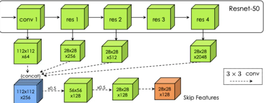
• The ResNet Architecture. In Kaiming He’s ResNet presentation he said: ”lower time complexity than VGG-16/19 so this change in the architecture allows a faster training. ” Apart from having less learnable parameters (VGG 16 has about 138 million parameters while ResNet has only 25.5 million) which is also better for training, the main reason that makes ResNet faster is that in VGG the first two layers apply convolution on top of the full 224x224 image (7x7 kernels) which is quite expensive while on Resnet only the first 3x3 kernel does. This simple computational case is enough for giving ResNet the victory in memory and time. Figure 3.7 shows an scheme of how the authors modified a ResNet with skip connections to obtain low-level and high-level combined features in two important tensors: the concat features of size (112,112,256) and the skip features of size (28,28,128). Those features are used aferwards to feed the First Vertex Network, the RNN, the Evaluation Network and the Graph Neural Network.

• Reinforcement Learning. On top of the CNN + RNN training that Polygon-RNN offered, in its improved version, the authors decided to train the outputs with the REIN-FORCE algorithm in order to make better decisions inside the 28x28 grid. In this training schedule, the reward function is the intersection over union (IoU) between the predicted polygon and the ground truth mask, so that in this schedule the goal is to grid-search over the 28x28 classes in order to improve vertex adjustments for larger IoU.

• The Graph Neural Network. Apart from the CNN + RNN and the reinforcement learning schedules, this model introduces a Graph Neural Network (GNN) that allows to scale from the 28x28 resolution back to 224x244 pixels from where it is easier to recover the original image in full resolution. The GNN interpolates the original polygon by creating a new vertex between every pair of existing vertices and then performs convolutions over the features of the vertices in order to decide which pixel is a better location for the vertex.

Figure 3.8: Scheme of evaluation network used in Polygon-RNN++. Figure origi-nally published in [1].

It is important to note that Polygon-RNN++ also includes attention and an evaluator network to predict better polygons. The evaluation network (Figure 3.8) is fed with the polygon mask prediction as well as the CNN features and the information of the last RNN hidden state. The evaluation network is trained to predict the Intersection over Union of the mask and can be used to maximize it. Its architecture is formed by 3x3 convolutions that convert from (28,28,128 + 16 + 1) to (28,28,16) and (28,28,1) that is finally connected with

(31)

3.2. POLYGON-RNN 31

Figure 3.7: Scheme of the modified ResNet used in Polygon-RNN as a CNN encoder for obtaining features. Figure originally published in [1].

Figure 3.9: Scheme of the architecture of the Polygon-RNN++ model. Figure originally published in [1].

a fully connected layer to one unique value which will be the IoU.

(32)

(33)

4.

A semi-supervised method for

im-age segmentation

This chapter can be considered the main chapter of this thesis. Under the different sections there will be presented the Cityscapes dataset, the Semi Supervised idea of the project along with the architecture and the models used, the supervised and unsupervised losses that have been implemented in order to train the model and finally some of the implementation details that have been chosen for obtaining the right performance.

4.1 The dataset: Cityscapes Dataset

In every Machine Learning or Deep Learning experiment, data is probably the most important thing. Not all methods can be used for any dataset and not all datasets allow the scientist to work with them in the same way. When facing a new dataset, a good data scientist must:

• Understandthe dataset. Because it is very likely that there are some particularities of the dataset such as class imbalance, noisy inputs or wrong labels that one is not aware of a priory.

• Decidewhich method will be used with such dataset. Sometimes, the task is defined but some models in the literature can perform that task and it is crucial to determine what model will better fit the data. On the other hand, sometimes the predifined final task is new and one has to develop the method from scratch. In those cases, this step can be done at the same time than the following ones.

• Preprocess the data according to the understanding of the dataset. It is very important to preprocess the data before using the chosen analysis method. Every method will work better under certain conditions such as normalized data, black and white images, ... Some of the most important preprocessing techniques are:

Checking for missing values Checking for categorical data Standardize the data

White the data and/or do a PCA transformation Split the data into train, validation and test sets

• Test and Visualize if the preprocessed dataset is intelligible and well prepared for the method chosen. Sometimes, after the preprocessing, some numerical errors might cause some disfunction in the posterior method. For this reason, I would say it is ”good praxis” to visualize the preprocessed data and ensure that no mistakes have been made (for instance, ensure that the values belong to the desired range, check that the images have been whitened...)

(34)

34 CHAPTER 4. A SEMI-SUPERVISED METHOD FOR IMAGE SEGMENTATION

Table 4.1: Number of object instances per class in each one of the different splits. Note that this is the same splitting published in [1]

Split Images Bicycle Bus Person Train Truck Motorcycle Car Rider Total Train 2711 3400 352 16452 136 455 657 24982 1575 48009 Val. 264 258 27 1462 32 27 78 1962 180 4026 Test 500 1129 98 3239 23 93 148 4517 537 9784

Figure 4.2: Example image of the Cityscapes Dataset. More concretely it was taken in the city of Weimar, federal state of Thuringia, Germany.

Figure 4.1: Map of the cities where have been taken the im-ages of the Cityscapes dataset

In this project, the dataset that has been used is the Cityscapes Dataset [9]. The Cityscapes Dataset contains 2975 training, 500 validation and 1525 test images with 8 semantic classes: bicycle, bus, person, train, truck, motorcycle, car and rider. All images contain annotations for all those classes and also for the following 11 categories: road, sidewalk, building, wall, fence, pole, traffic light, traffic sign, vegetation, terrain and sky. Figures 4.2 and 4.3 show a couple of examples of how are the annotated images of the dataset. All the images were taken in different cities of the center of Europe, more concretely Germany and Switzerland. Figure 4.1 shows a map with all the locations where pictures were taken. Note that for this project there has been only the possibility to work with the train and validation sets because the test images are private and cannot be downloaded. According to the available data, the splitting that we use is the following: we divide the 2975 training images into 2711 for training and 264 for validation while we keep the 500 for testing. The same split was used in [1]. Table 4.1 describes how many object instances are in every one of the splits used in the experiments.

4.1.1 Cityscapes preprocessing

The final goal of this project is predicting masks as accurate as possible of the 8 classes of the Cityscapes dataset with as less labeled data used as possible. Since the same dataset and splitting was recently used in [1], we also preprocess the data in the same way:

(35)

4.1. THE DATASET: CITYSCAPES DATASET 35

Figure 4.3: Example image of the Cityscapes Dataset. More concretely it was taken in the city of M¨unster, in North Rhine-Westphalia, Germany

1. Take every instance of one of the 8 classes and crop it from the image.

2. Remove some noisy annotated crops that could be present such as those that the area is less that 100 pixels.

3. Add some random context (i.e. margins) to the cropped image in order to obtain the instance centered but also to include background in the image.

4. Resize the cropped image to 224x224 pixels. 5. Resize the annotated mask and to 224x224 pixels.

6. Prepare pixel maps that contain information about where the vertices and edges of the mask could be.

7. Remove all the labeling from some of the images according to the desired experiment. In this step we remove every annotation that was present in the dataset and we only keep the 224x224 raw image.

8. Feed the network with batches of some labeled and some unlabeled images.

4.1.2 Cityscapes benchmark

As complimentary imformation, Table 4.2 presents some of the current benchmarks of pixel segmentation among the 8 classes and the 11 categories. To assess performance, in Cityscpaes [9] use the standard Jaccard Index, also known as the PASCAL VOC intersection-over-union metric [10]:

IoU = T P

T P +F P +F N (4.1)

where TP, FP, and FN are the numbers of true positive, false positive, and false negative pixels, respectively, determined over the whole test set. Note that pixels labeled as void do not contribute to the score.

In order to solve the problem that the global IoU measure is biased toward object instances that cover a large image area, what Cityscapes proposed is to additionally evaluate the semantic

(36)

Table 4.2: Cityscapes Pixel Segamentation Benchmark.

Model Name IoU class iIoU class IoU category iIoU category

iFLYTEK-CV 83.6 64.7 92.1 82.3 NV-ADLR 83.2 64.2 92.1 82.2 Tencent AI Lab 82.9 63.9 91.8 80.4 DRN CRL Coarse 82.8 61.1 91.8 80.7 DPC 82.7 63.3 92.0 82.5 SRC-B-MachineLearningLab 82.5 60.7 91.8 81.5 RelationNet Coarse 82.4 61.9 91.8 81.4 DeepLabv3+ 82.1 62.4 92.0 81.9 Auto-DeepLab-L 82.1 61.0 91.9 82.0

labeling using an instance-level intersection-over-union metric. For each type of instancei, iIoU = iT P

iT P +F P +iF N (4.2) where again iTP, FP, and iFN denote the numbers of true positive, false positive, and false negative pixels, respectively but in contrast to the standard IoU measure, iTP and iFN are computed by weighting the contribution of each pixel by the ratio of the class’ average instance size to the size of the respective ground truth instance. Note that since the methods only yield a standard per-pixel semantic class labeling as output, the false positive FP pixels are not associated with any instance and thus do not require normalization. The final scores, iIoUcategory and iIoUclass, are obtained as the means for the two semantic granularities.

I would like to point out in particular one method that is present in 4.2: DeepLabv3+ [7]. I would like to address the reader to that bibliography to further improve knowledge of pixel segmentation since both methods improved state-of-the-art performance in diverse tasks and datasets and allow the reader to understand how pixel segmentation can be trained not only on 8 classes of objects but on hundreds using tricks as encoding and decoding, atrous convolutions and conditional random fields and obtain such as good results as shown in Figure 4.4.

Figure 4.4: Example output of some masks using Deeplabv3+ in the ImageNet dataset

4.2 The Semi-Supervised Approach

This section presents the problem that I faced at the beginning of this project as well as the solution that I propose to solve it. At the beginning of my research internship, I was told that some previous work in the Vector Institute laboratory was on the Cityscapes Dataset [9] (namely

(37)

4.2. THE SEMI-SUPERVISED APPROACH 37

Figure 4.5: Example of an input image from the Cityscapes Dataset. This input has been cropped from a bigger image that contains a lot of entities and has been resized to 224x224 pixels.

both Polygon-RNN and Polygon-RNN++ [1, 5]) and that also in the field of Deep Learning, some relevant papers in Semi-Supervised Learning had been published. I started questioning if it was possible to combine those ideas and try to use a semi-supervised approach for image segmentation, and more concretely in the Cityscapes Dataset.

On the next pages, I would like to present the idea of how those ideas can be combined, the losses that we have designed for training a model to understand the unlabeled data, the architecture of the model that we used for training and finally the schedule and hyper-parameters that we used for training.

4.2.1 The idea

To train in a Semi-Supervised way, the most important problem to solve is how one will use the unsupervised data. This is a non-trivial question to answer in a segmentation framework where the labeled data are pixelwise masks of the objects given an image but for the unlabeled data there’s only the raw image without any annotation. More concretely, in the processed Cityscapes dataset [9], which was already used in [1, 5] the input for any model is always a crop from a region containing one entire entity (car, person, bicycle, ...) and maybe partially regions of other images. Figure 4.5 shows an example of an input image which has a resolution of 224x224 pixels. In the Cityscapes dataset, it is possible to have pixelwise ground truth for vertices, edges and mask of the input image. Figure 4.6 represents the ground truth that is available for the input image of Figure 4.5.

With those ideas in mind, in a Supervised Framework, it is possible to use a pixelwise binary cross-entropy to supervise the edges, vertices and mask prediction. Assume that the ground truth maps are threee pixel maps of 224x224 resolution containing a value of 1 when the pixel is white (i.e. it is a vertex or forms part of an edge or mask) and 0 otherwise (represented by black in Figure 4.6). Also assume that the network produces three pixel map outputs also at a 224x224 resolution with values between 0 and 1 expressing the confidence of that pixel to be triggered in that map (this is typically done using a sigmoid function per pixel as a last layer of the network). Consider thatq(i, j)k is the ground truth value for the pixel of the ith row and

the jth column of the map k, where for instance k= 1 will denote verices, k= 2 edges and k= 3 mask. Let’s definep(i, j)k as the predicted probability for the same pixel, then equations

(38)

Figure 4.6: Examples of the Ground Truth Data of the Cityscapes Dataset. Those three images can be used as ground truth for the input image in Figure 4.5

be used when a ground truth map is available, and hence in a semi-supervised approach a new loss will have to deal with the unlabeled data.

L_bce(q, p) =−q·log(p)−(1−q)·log(1−p) (4.3)

L_BCE = 3 X k=1 1 2242 224,224 X i=1,j=1

L_bce(q(i, j)k, p(i, j)k) (4.4)

Inspired by the papers on Semi-Supervised Learning for Image Classification [16, 19, 22, 29], the main idea of a semi supervised approach is forcing the network to be consistent with its predictions of the unlabeled data. In a regime such as image segmentation, I personally think that this consistency can be applied in two different ways. On the one hand, it is possible to evaluate twice the same input and penalize the network if it’s not confident on giving the same result twice (note that if the network contains stochasticity, either in the input or in some layers, this is not trivial), this can be thought as being consistent within every pixel map. On the other hand, since we are producing output maps of vertices, edges and masks and there is a strong relation between those maps (the edge map should be the external pixels of the mask map and the vertices map should contain vertices that are extremes of the edge map), one could take leverage by penalizing a non-consistent output.

A lot of methods exist in the literature to extract edges or vertices form a mask but I would like to focus on the Canny edge detector [4] and the Harris corner detector [12].

The Canny Edge Detector.

Traditionally, the Canny edge detection algorithm can be divided into 5 different steps:

• Apply aGaussian filter to smooth the image in order to remove the noise. Matrices in 4.5 show the typically used 3x3 and 5x5 Gaussian filters. Those filters take into account the intensities of the neighbours of a pixel in order to smooth the whole image and hence

(39)

4.2. THE SEMI-SUPERVISED APPROACH 39 easy the next steps.

1 6    0 1 0 1 2 1 0 1 0   , 1 159         2 4 5 4 2 4 9 12 9 4 5 12 15 12 5 4 9 12 9 4 2 4 5 4 2         (4.5)

• Find the intensity of the gradients of the image. This can be done using convolutional kernels that approximate the limitf0(x) = limh→0(f(x+h)−f(x−h))/h. In 4.6 are the typical 3x3 gradient filters.

Gx=    0 0 0 1 0 −1 0 0 0   , Gy =    0 1 0 0 0 0 0 −1 0    (4.6)

• Apply non-maximum suppression to get rid of false positive responses that are fired during edge detection. This is done in order to obtain thinner edges.

• Applydouble thresholdto determine the potential edges. The regions of the image that are more likely to be an edge, will always have a response bigger than a certain threshold. • Finally it is also possible to suppress all the remaining edges that are weak and

not connected to strong edges.

The Harris Corner Detector.

As the Canny edge detection algorithm, the Harris corner detector also can be thought as a 5-step process:

• Color to grayscale. This algorithm works using only one channel with values between 0 and 255.

• Compute the spatial derivatives. This step is analogus to the first two steps of the Canny edge detector method. One should apply convolutional filters to first obatain an smoothed image and then obtain the gradient intensity mapsIx and Iy.

• Build a 2x2tensor for every pixelusing the formula in equation 4.7.

M(i, j) = "

I_x2(i, j) Ix(i, j)Iy(i, j)

Ix(i, j)Iy(i,j) Iy2(i, j)

#

(4.7)

• Calculate theHarris response. This is calculating the minimum eigenvalue of the matrix for every pixel. We know that a point is a corner if there are high perturbations in both directions and hence if and only if both eigenvalues are high and positive. After calculating the minimum eigenvalue per pixel using the approximation in equation 4.8, there will be corners for all the values that have a value of λmin higher than certain threshold.

λmin ≈

λ1λ2 (λ1+λ2)

= det(M)

(40)

40 CHAPTER 4. A SEMI-SUPERVISED METHOD FOR IMAGE SEGMENTATION • End the process performing aNon-maximum suppression as in the Canny edge

detec-tor.

Using the Canny Edge Detector [4] and the Harris Corner Detector [12], it is possible to obtain a map of the edges and a map of the vertices using a mask. Hence, the idea of this project lies in applying a consistency loss between the edge map predicted by the network and the obtained by performing one of those detection methods on top of the predicted mask map. This is a fully unsupervised approach, like a regularization method that just takes into account the predictions and penalizes the model whenever they are not consistent.

When the input data is supervised, it is also possible to use this consistency between the ground truth maps and the predictions (i.e. Applying the detectors on the ground truth mask and comparing against the predicted edges/vertices and/or applying the detectors on the predicted mask and comparing against the ground truth edges/vertices.

On top of that idea, it is also interesting the fact that the number of vertices/edges of the prediction cannot be extremely big. For this reason, it is also possible to include another loss that penalizes the fact that too many or too less vertices are predicted. This is typically done in the supervised data using the weighted binary cross entropy which is very similar to the binary cross entropy (Equation 4.3) but weighting by an alpha parameter that typically is inversely proportional to the quantity of ground truth positive predictions (Equation 4.9). In our case, we propose to penalize a big number of predicted edges/vertices by the difference against the allowed maximum or a low number by the difference against the allowed minimum.

L_wbce(q, p) =−α q log(p)−(1−α)(1−q) log(1−p) (4.9)

4.2.2 The losses

Assume thatx is the Cityscapes input data and let’s define XL andXULas the labeled and

unlabeled sets respectively. Assume thatp(x, y)m, p(x, y)e, p(x, y)v are the the mask, edges and

vertices predicted pixel-wise probability maps for one instance, (x, y)∈ {224}x{224}. Assume also that ˆy are predicted probabilities for the instance being in each one of the 8 classes of Cityscapes. Finally, assume thatq(x, y)m, q(x, y)e, q(x, y)v andy are the corresponding ground

truth labels. In the following, there are presented all the losses that are used during the semi-supervised training where the data is processed with mini-batchesB.

1. Binary Cross Entropy (BCE).The BCE is used on the labeled fraction of the mask predictions. Equation 4.10 shows the loss for each mini-batch:

L_BCE =            1 |B∩XL|·2242 224,224 X i=1,j=1 x∈XL∩B

Lbce(q(i, j)m,x, p(i, j)m,x)) ifB∩XL6=φ

0 ifB∩XL=φ

(4.10)

2. Weighted Binary Cross Entropy (WBCE).The WBCE is used on the labeled fraction of the edges and vertices predictions where there is a huge class imbalance between positives and negatives. Equation 4.11 shows the loss for each mini-batch where k can be both

(41)

4.2. THE SEMI-SUPERVISED APPROACH 41 edges eor verticesv: L_{W BCE} =            1 |B∩XL|·2242 224,224 X i=1,j=1 x∈XL∩B

Lwbce(q(i, j)k,x, p(i, j)k,x)) ifB∩XL6=φ

0 ifB∩XL=φ

(4.11)

3. Classification Loss (CL). The classification loss is used to help the network identify what kind of instance it is trying to segment. It is a loss only used on the labeled data and it is a cross entropy between the predicted classes ˆy and the ground truth labels as one-hot encoding vectorsy (Equation 4.12).

LCL=        X x∈B∩XL 8 X i=1 −y_ixlog(ˆyx_i) ifB∩XL6=φ 0 ifB∩XL=φ (4.12)

4. Consistecny Loss (C). The consistency loss is directly a squared difference between two predictions of the same input. This is analogous as the procedure done in the Pi Model [16] and the loss is explicitly shown in equations 4.13 and 4.14 whereq1 and q2 are two predictions and k can be masks m, edges eor verticesv:

Lc(q1, q2) = 1 2242 224,224 X i=1,j=1 (q1−q2)2 (4.13) L_C = 1 |B| X x∈B L_c(q1,k,x, q2,k,x) (4.14)

5. Consistency between Mask and Edges (CME). The CME loss takes into account how consistent is the predicted edge map with the predicted mask. In order to do so, for the unlabeled data the penalization is a consistency loss between the predicted edges and the Canny detector map over the predicted mask. Nevertheless, on the labeled data it is possible to use this consistency between one of the predicted maps and one ground truth map. This loss is shown in equation 4.15 as a sum of three consistency losses, where Can is understood as the operation that using Canny edge detection results as the map of the detected edges over an image.

L_{CM E} = X x∈B∩XU L L_c(Can(qm), qe) + X x∈B∩XL (L_c(Can(pm), qe) +Lc(Can(qm), pe)) (4.15)

6. Consistency between Mask and Vertices (CMV).The CMV loss works exactly as the CME loss but taking into account the consistency between mask and vertices. Equation 4.16 shows explicitly the loss. Note that Har denotes the operation that using Harris corner detection results as the map of the detected vertices over an image.

LCM V = X x∈B∩XU L Lc(Har(qm), qe) + X x∈B∩XL (Lc(Har(pm), qe) +Lc(Har(qm), pe)) (4.16)

(42)

Figure 4.7: Scheme of the modified ResNet-50 used as a backbone model for this project.

7. Some Vertices (SV).The SV loss encourages the network to predict a number of vertices and edges over a certain range. Let’s definevmin andvmax as the minimum and maximum

values of vertices that we want a prediction to have andemin andemax the same for edges.

Equations 4.17 and 4.18 show the SV loss where k can be used for either vertices v or edgese. Qk= 224,224 X i=1,j=1 q(i, j)k1q(i,j)>0.5 (4.17) L_SV =          kmin−Qk ifQk< kmin 0 ifQk∈[kmin, kmax] Qk−kmax ifQk> kmax (4.18)

A loss composed by the sum of all those losses is used during training time. Equation 4.19 shows this total loss. The weight hyper-parameters that are used during training are the following: λ1= 1000,λ2 = 100,λ3 = 10 and λ4 = 0.1.

L_{T OT AL}=λ1(LBCE+LW CE) +λ2(LC+LCL) +λ3(LCM V +LCM E) +λ4LSV (4.19)

4.2.3 Our backbone model

Since the code of this project was build on top of the inherited Polygon-RNN++ code [1], the main experiments and all the testing research was done with a ResNet-50 modified model very similar to the one they used (See Figure 4.7 for an orientating scheme). We keep the same structure with skip conections but we change the last layers:

• Keep exactly as in PolygonRNN++ the conv1, res1, res2, res3 and res4 layers of the ResNet.

• Concatenate the features obtained at the biggest scale (112x112 pixels) to obtain a tensor of size (112,112,256).

• Use two 3x3 convolutional layers of 128 layers mantaining the spatial dimension.

• Upsample the final features to obtain a (224,224,128) tensor that will be used to predict the mask, edges, vertices (through a 3x3 kernel) and the classes of the instance (with a fully connected).

Note that all the losses should be independent of the backbone model since they only require the prediction pixel-wise maps. Nevertheless, it is future work test that this theoretical behaviour will allow to obtain good results with all kind of different backbones.

(43)

4.3. IMPLEMENTATION DETAILS AND TRAINING SCHEDULE 43

4.3 Implementation Details and Training Schedule

During training time, the first step we perform is preparing a Dataloader with the number of labels proposed for the experiment. In the next section, we will present results with 2000, 4000, 6000, 80000 and 10000 labels. We chose 16 to be the mini-batch size and at every forward pass we compute all 7 losses and then decide which combination will be backpropagated following the experiment instructions.

We have chosen the learning rate to start at 0.0001 and decrease by a factor of 0.3 every 3 epochs. We also include the same ramp schedule than in [16] multiplying the unsupervised losses by 0.01 on the first epoch and increasing gradually until 1 on the sixth.

We have chosen to preserve the same hyper-parameters for all experiments except for the period of decreasing the learing rate which we scale inversely proportionally to the amount of labeled data in the supervised experiments.

The code and the training schedule will be released at http://github.com/jordifortuny/

(44)

(45)

5.

Experiments and Results

In order to test the improvement of the losses, we evaluate some experiments on the Cityscapes Dataset [9]. More concretely, this section presents ablation studies that show how the accuracy (Intersection over Union or F-score) increases when adding different combinations of our losses. There are also included some comparisons between the best Semi-Supervised models versus models that have been only supervised on different regimes. Moreover, we also show some visual results of the semi-supervised models that prove that gain better understanding over the dataset classes.

Table 5.1 and Images 5.1, 5.2 and 5.3 show a comparison between the best trained models on different data regimes on the Cityscapes Dataset. The models have been trained and tested using 5%, 10%, 15%, 20% and 25% of the data. We considered that testing the model on both low data regimes (5%) and high data regimes (25%) was a fair study to show how the model performs. As one can see, with only 5% of the data labeled, our semi-supervised model achieves an outstanding 93% of the fully supervised Intersection over Union. Note that when one adds more data, the results are better and reach about 98% of the fully supervised approach using only 25% of the data. It is also important to note that in all experiments the semi-supervised models improve the only supervised models by at least 2 points.

0 25 50 75 100 55 60 65 70 75 Labeled Data (%) Mean IoU (%) All Labels Semi-Supervised (Ours) Supervised

Figure 5.1: IoU when different data regimes are labeled. The Semi-Supervised Model outperforms the only supervised model by more than 4 points on low labeled regimes and by approximately 2 points on high labeled regimes