Working Paper Series
WP 2011-6
School of Economic Sciences
Commitment in Environmental
Policy as an Entry-Deterrence Tool
By
Ana Espinola-Arredondo and Felix
Munoz-Garcia
Updated
February
201
2
Commitment in Environmental Policy as an
Entry-Deterrence Device
Ana Espínola-Arredondo
School of Economic Sciences Washington State University
Pullman, WA 99164
Félix Muñoz-García
ySchool of Economic Sciences Washington State University
Pullman, WA 99164 February 29, 2012
Abstract
This paper investigates under which conditions governments strategically commit to strin-gent environmental policies in order to balance market power and the damages emerging from the externality. We compare social welfare under two policy regimes: a ‡exible and in‡exible environmental policy. Our results show that an in‡exible policy becomes socially optimal when its associated welfare loss, due to a stringent fee across time, is smaller than its welfare gain, which arises from an improved environmental quality since only one …rm operates in the mar-ket. Otherwise, the regulator optimally chooses a ‡exible environmental policy which cannot credibly deter entry. In addition, we demonstrate that the incentives of the social planner and incumbent are not necessarily aligned regarding policy regimes. In particular, under certain conditions the regulator …nds socially optimal to commit to an in‡exible policy, which deters entry, whereas the incumbent would actually prefer a ‡exible policy that attracts entry.
Keywords: Entry deterrence; Emission fees; Perfect commitment. JEL classification: L12, L5, Q5, H23.
Address: 111C Hulbert Hall, Washington State University, Pullman, WA 99164. E-mail: [email protected].
yAddress: 103G Hulbert Hall, Washington State University. Pullman, WA 99164-6210. E-mail: [email protected].
1
Introduction
Recent studies have stressed the potential e¤ects that environmental policy has on market structure and competition. These studies can be grouped according to the primitive reason that explains why environmental regulation hinders entry and/or limits competition upon entry. On one hand, Ryan (2011) and OECD (2006) show that certain types of environmental regulation increase the initial investment that entrants must incur in order to start operating in an industry, thus reducing entry.1 On the other hand, similar studies demonstrate that environmental policies impose cost di¤erentials among …rms. Speci…cally, these papers identify the presence of strong economies of scale in the compliance of environmental policy, entailing a cost di¤erential between incumbents and entrants if their scale of operations di¤ers.2 Furthermore, such cost di¤erential can be further augmented since environmental policy often places a heavier burden on new pollutant sources than on the incumbents’.3
This paper investigates the e¤ect of environmental policy on market entry, showing that environ-mental regulation may be detrienviron-mental for competition,even in the absence of the above arguments. Our results therefore emphasize that the potential adverse e¤ects of environmental regulation are not restricted to industries with particular production processes, or to markets where environ-mental policy exhibits administrative economies of scale, or settings where incumbent and entrant …rms are di¤erently a¤ected by regulation. Instead, our …ndings highlight the fact that such entry-deterrence e¤ects can be extended to industries where …rms are symmetric in costs and they are similarly a¤ected by environmental policy.
In particular, our study considers a social planner who imposes emission fees on an industry, initially monopolized by an incumbent …rm, and where an entrant may decide to enter afterwards. For generality, we allow the regulator to choose among two policy regimes: a ‡exible policy, where authorities adapt the stringency of the emission fee if the number of polluting …rms operating in the industry changes, and an in‡exible policy, whereby the regulator does not have the ability to rapidly revise his environmental policy if the market structure changes. Since under an in‡exible policy initial fees are still enforced in the post-entry game, this policy can attract or deter entry when the regulator commits to a relatively low or high fee, respectively. In contrast, ‡exible policy cannot credibly deter entry, since the regulator has incentives to revise emission fees if entry ensues. We …rst show that, under a ‡exible policy, the regulator imposes more stringent fees to duopolists than to the incumbent monopolist; as in Buchanan (1969). Under an in‡exible policy, by contrast, the social planner must commit to a single emission fee, thereby producing ine¢ ciencies in either one or both periods. Under certain conditions, however, the regulator can improve social welfare
1
In particular, Ryan (2011) found that the Clean Air Act Amendments of 1990 increased the sunk entry cost by 35% in the market of Portland cement. He argues that, despite the increased pro…tability in this sector, few entrants chose to enter the industry.
2
See, for instance, Ungson et al. (1985), Brock and Evans (1985), Dean et al. (2000) and Helland and Matsuno (2003). In this line of work, Monty (1991) and Dean and Brown (1995) report learning-by-doing e¤ects in the com-pliance of environmental regulation, emphasizing the cost advantage of incumbent …rms who are already familiarized with the administrative details of the policy.
3
by strategically committing to a signi…cantly high fee that deters entry. In particular, relative to a ‡exible policy, the imposition of a stringent in‡exible fee produces two opposite e¤ects: …rst, it reduces monopoly output during both periods, but second, it improves environmental quality by limiting pollution. When the latter e¤ect dominates the former, overall welfare increases, and therefore entry-deterrence becomes socially optimal. This occurs when entry costs are high, since in this setting entry can easily be deterred by setting a relatively low fee which does not entail signi…cant welfare losses. Entry deterrence is further facilitated when the environmental damage from pollution is relatively high. Indeed, entry-deterrence reduces output, which entails an envi-ronmental bene…t from a lower level of pollution that is further emphasized as it becomes more damaging. Otherwise, entry deterrence becomes extremely costly and/or does not entail signi…cant environmental bene…ts. Attracting entry is thus socially optimal and the regulator selects a ‡exible environmental policy.
Our results hence identify under which conditions the regulator might strategically commit to a relatively stringent environmental policy that, despite hindering the entry of additional …rms in subsequent periods, can ultimately lead to welfare improvements. Such equilibrium outcome, how-ever, assumes that regulatory authorities can directly modify the ‡exibility of their environmental policies. If such degree of ‡exibility is given by the country’s institutional context, our results suggest that countries where environmental regulation slowly adapts to changes in the regulated industry could be unintentionally hindering entry. The use of in‡exible policy, however, would not be necessarily suboptimal if, speci…cally, entry costs and the environmental damage from pollution are relatively high.4
Finally, we investigate whether the incumbent’s pro…ts are positively a¤ected by emission fees that deter entry. An in‡exible policy allows the incumbent to maintain its monopoly power, but reduces pro…ts across time. We show that, when entry is deterred by setting a low in‡exible emission fee (i.e., entry costs are large), the incumbent’s bene…ts from monopolizing the industry outweigh the costs from bearing a stringent regulation, and hence the incumbent prefers an in‡exible policy. In contrast, when entry-deterrence is more di¢ cult (small entry costs), emission fees become more substantial; implying that the incumbent prefers a ‡exible policy even if it attracts entry. We furthermore demonstrate that the regulator’s and incumbent’s interests are not necessarily aligned. In particular, when the regulator …nds entry-deterrence socially optimal, the incumbent also favors such policy if the emission fee it bears is relatively small, but opposes it otherwise. Our results hence provide an important distinction often overlooked by critics of environmental policy, who regard it as a tool governments use to protect domestic monopolies from entry and competition. Indeed, our predictions show that the interests of regulatory agencies and incumbent …rms might be aligned, but only when entry is relatively easy to deter. Otherwise, the incumbent may actually prefer that the regulator practices less entry deterrence.
4That is, even if the regulator had the ability to choose a policy regime (‡exible or in‡exible policies), he would
prefer an in‡exible policy. Note that if, in contrast, countries’ given institutional setting is relatively ‡exible, our results predict that such regulation would attract additional …rms in the industry, yielding optimal social welfare if entry costs and the environmental damage from pollution are su¢ ciently low.
Related literature. Our paper contributes to three main areas of the literature: that analyzing the e¤ects of environmental policy on entry and competition; that considering the optimal use of commitment in contexts where regulators face time-inconsistency problems; and the literature that examines entry-deterrence in industrial economics. As suggested above, our paper o¤ers a new setting where environmental regulation can serve as an entry-deterrence device, even in the absence of any of the arguments commonly used in the literature: economies of scale or learning-by-doing e¤ects in the compliance of regulation, cost-di¤erentials emerging from environmental policy, etc.
Moreover, the paper contributes to the literature comparing ‡exible and in‡exible policies. Since the initial work by Kydland and Prescott (1977) and Barro and Gordon (1983), several papers examined perfect commitment in monetary policy, Chang (1998) and Alvarez et al. (2004), in capital tax policy, Chamley (1986) and Benhabib et al. (2001), or in both, Dixit and Lambertini (2003). These papers consider a context where in‡exible policies can be welfare improving under certain conditions. Commitment in monetary policy, for instance, a¤ects agents’ expectations of in‡ation thereby changing their current economic decisions. This paper similarly identi…es how commitment in environmental policy can be used to a¤ect the entrant’s expectations about its future pro…tability, deterring entry in certain contexts and increasing overall welfare.5
Finally, our paper relates to the literature on entry-deterrence games initiated by Bain (1956) and Sylos-Labini (1962) for one incumbent and extended by Gilbert and Vives (1986) to several incumbents, by Waldman (1987) to settings of incomplete information, and by Kovenoch and Roy (2005) to product-di¤erentiated markets.6 A common assumption in these models is that the in-cumbent …rm commits to a particular level of output which, if su¢ ciently large, may deter entry from potential entrants. In our paper, the incumbent …rm cannot commit its future production decision, whereas the regulator can set a constant emission fee across periods, thereby using envi-ronmental policy as an entry-deterrence tool in certain contexts. An important di¤erence of our model is that the regulator deters entry in settings where the incumbent would have preferred entry to ensue. Because the literature on entry-deterrence often abstracts from the regulatory context in which …rms operate, entry is only deterred if the incumbent seeks to discourage the newcomer. Our results, in contrast, predict settings where entry deterrence is favored by the incumbent, but also contexts where it is actually opposed by the incumbent …rm.
The next section describes the model and time structure of the game. Section 3 examines the second-period game, while section 4 investigates the …rst-period game both with ‡exible and in‡exible policies. Section 5 compares the overall social welfare ensuing from the selection of di¤erent environmental policies. At the end of section 5 we evaluate the incumbent’s pro…ts under 5Ko et al. (1992) compare ‡exible and in‡exible environmental policies under a complete information context
where a single incumbent produces stock externalities, i.e., pollution that does not fully dissipate across periods, without allowing for potential entry. Because entry cannot occur in their setting, the optimal policy path across periods mainly depends on the dissipation rate. In our model, in contrast, pollution fully dissipates across periods but entry may occur, thus a¤ecting the social planner’s optimal policy path with and without commitment.
6
In a reinterpretation of the quantity commitments considered in these papers on entry-deterrence, Spence (1977), Dixit (1980), Ware (1984) and Fudenberg and Tirole (1984), assume that incumbent …rms commit to an investment in capacity, providing similar results.
‡exible and in‡exible policies, and section 6 concludes.
2
Model
Consider an entry game with a monopolist incumbent, an entrant who decides whether or not to join the market and a regulator who sets an emission fee per unit of output.7 The incumbent’s constant marginal costs are either highHor lowL, i.e.,cHinc> cLinc 0, where subscriptincdenotes the incumbent. In particular, we study a two-stage complete-information game with the following time structure:
1. In the …rst stage, the regulator chooses between an in‡exible environmental policy (setting a constant fee t across time); and a ‡exible policy, i.e., setting fee t1 (t2) in the …rst (second)
period.
2. Given the …rst-period environmental policy, the incumbent responds selecting an output level, i.e., qK(t) under an in‡exible policy or qK(t1) under a ‡exible policy, where K = fH; Lg
represents the incumbent’s type.
3. In the second-period game, the entrant decides whether to enter the industry after observing the regulator’s choice of environmental policy and the incumbent’s marginal costs.
4. The regulator maintains his environmental policy t if he is committed to a constant fee. Otherwise, he revises the policy fromt1 tot2. In addition:
(a) If entry does not occur, the incumbent responds producing a monopoly outputxK;N Einc (t)
under an in‡exible policy and xK;N Einc (t2) under a ‡exible policy; where superscript NE
denotes no entry.
(b) Similarly, if entry ensues both …rms compete as Cournot duopolists, producing xK;Einc (t)
andxK;Eent (t)under an in‡exible policy, andxK;Einc (t2)andxK;Eent (t2)under a ‡exible policy;
where superscript E represents entry and subscript ent denotes the entrant.
In the following section we examine fees and output levels in the second-period game, as well as the resulting social welfare in equilibrium. Afterwards we analyze the …rst stage, and …nally compare social welfare under ‡exible and in‡exible policies.
3
Second-period game
Flexible policy. Let us next examine the subgame where the regulator selects a ‡exible
environ-mental policy. 7
As described below, our model allows for emissions to be a convex function of output, embodying not only cases in which the relationship between output and emissions is proportional, but also cases in which such relationship is increasing.
No entry. If entry does not occur, the incumbent’s pro…ts when facing a given fee t2 are
K;N E
inc (xinc) p(xinc)xinc cKinc+t2 xinc, whereK =fH; Lg, and the inverse demand function
p(xinc)is linear in output and satis…es p0(xinc)<0 andp(xinc)> cKinc for allxinc. The regulator’s
social welfare function in the second period is
SW2K;N E CS(xinc) + K;N Einc (xinc) +TK;N E d(xinc), (3.1)
where CS(xinc)
Z xinc
0
p(x)dx p(xinc)xinc represents the consumer surplus for a given output
xinc. The parameter denotes the weight that the social planner assigns to consumer surplus and
2[0;1]. In addition, TK;N E is the tax revenue under no entry, and function d(xinc) represents
the strictly convex environmental damage from output, where d0(xinc) > 0 and d00(xinc) > 0.8
Furthermore, we assume that the marginal environmental damage satis…es p(0) cKinc > d0(0), which ensures that it is socially e¢ cient to produce the …rst unit of output. The regulator seeks to induce the socially optimal output xK;N ESO which solvesM BK;N E(x
inc) =M DN E(xinc), where
M BK;N E(xinc) (1 )p0(xinc)xinc+p(xinc) cKinc (3.2)
represents the marginal bene…t of additional output on consumer and producer surplus, whereas M DN E(xinc) d0(xinc) denotes the marginal environmental damage of output. The regulator
then imposes an emission fee tK;N E2 = M PincK;N E(xK;N ESO ) on monopoly output in order to induce the production level xK;N ESO in the second period, where M PincK;N E(xinc) represents the marginal
pro…ts of increasingxinc given no entry.9
Entry. If entry occurs, …rms compete as Cournot duopolists in the second period. The pro…t functions for the incumbent and entrant are
K;E
inc (xinc; xent) p(X)xinc cKinc+t2 xinc and K;Eent (xinc; xent) p(X)xent (cent+t2)xent
(3.3) whereX =xinc+xent represents the aggregate output level, superscript E denotes entry and cent
is the entrant’s marginal cost wherecent =cHinc. The regulator’s social welfare function is
SW2K;E CS(X) +P S(X) +TK;E d(X). (3.4) whereP S(X) K;Einc (xinc; xent) + K;Eent (xinc; xent) F. The regulator aims to induce the aggregate
8
Note that this damage function allows for aggregate emissions to be a convex function of output, and in turn, overall damage from pollution to be a convex function of aggregate emissions. That is, emissions can be represented asei=f(xinc), wheref( )is weakly convex inxinc, and environmental damage as d(xinc) =g(f(xinc)), whereg( )
is also a weakly convex function in emissions.
9Appendix 1 shows that such an emission fee exists both under entry and no entry. In addition, note that when
social welfare does not include consumer surplus, = 0, the optimal tax leads the incumbent to fully internalize the environmental damage of her output decision. However, when >0, the relative value of consumption increases, which implies a lower optimal taxtK;N E2 . Therefore, the monopolist only internalizes a fraction of her environmental damage.
socially optimal output XSOK;E that solvesM BK;E(X) =M DE(X), where
M BK;E(X) (1 )p0(X)X+p(X) cKinc (3.5) and M DE(X) d0(X). Hence, the emission fee tK;E2 that induces aggregate output XSOK;E is tK;E2 = M PjK;E xK;Ej;SOjxK;Ek;SO for all …rm j = finc; entg and k 6= j, where M PjK;E xjjxK;Ek;SO
denotes the marginal pro…t that …rmjobtains by increasing its duopoly output given that its rival kproduces the socially optimal output10 xK;Ek;SO.
To make entry decision interesting, we consider that when the incumbent’s costs are low, entry is unpro…table, i.e., the entrant’s duopoly pro…ts, L;Eent(t), lie below his …xed entry costF, L;Eent(t)< F, for any emission fee t. Hence, the entrant stays out even when emission fees are absent, i.e.,
L;E
ent(0)< F. In contrast, when the incumbent’s costs are high, entry is pro…table in equilibrium
both under the ‡exible and in‡exible fee. As section 4.2 shows, the ‡exible fee is more stringent than the in‡exible tax, thus implying that entrant’s pro…ts are lower when the environmental policy is ‡exible. Therefore, the entrant joins the market if H;Eent (tH;E2 ) > F.11 Entry, however, becomes unpro…table if fees are su¢ ciently high. That is, H;Eent (t) decreases in t and satis…es H;Eent (t) F for all feest t. For compactness, we refer tot as the “entry-deterring fee.”
In‡exible policy. Under an in‡exible policy, …rms face the same constant feetthat the regulator
selects in the …rst-period game, producing outputxK;N Einc (t)in the case of no entry andxK;Ej (t)for any …rmj=finc; entgin the case of entry. Hence, we analyze the regulator’s setting of an optimal in‡exible policy in our discussion of the …rst-period game.
4
First-period game
4.1 Flexible policy
The regulator seeks a …rst-period output q that maximizes social welfare. Speci…cally, this occurs when the socially optimal output under monopolyqKSOsolvesM BK;N E(q) =M DN E(q). Analogous to the no-entry case in the second stage, emission fee tK1 = M PincK qSOK induces the monopolist to produce qK
SO. Consequently, this fee coincides with that under monopoly in the second period,
tK1 =tK;N E2 . Let SWL;N E tL1; tL;N E2 denote the overall social welfare across both periods when entry does not ensue since the incumbent’s costs are low, and the regulator sets tL
1 and t
L;N E
2 fees
in the …rst and second period, respectively. Similarly, let SWH;E tH1 ; tH;E2 represent the social welfare when entry occurs given that the incumbent’s costs are high, and the regulator sets fees
1 0This implies that, when the incumbent’s costs are high, in order to …nd feetH;E
2 and individual output levelsx
H;E j;SO
andxH;Ek;SO, the social planner must simultaneously solve xH;Ej;SO+xk;SOH;E =XSOH;E and tH;E2 =M P
H;E j x H;E j;SOjx H;E k;SO
for both …rmsj=finc; entg.
1 1
Note that these conditions on entry costs, i.e., H;Eent (t H;E
2 )> F >
L;E
ent(0), also satisfy the standard assumption
in entry-deterrence models where regulation is absent, in whichF satis…es H;Eent (0)> F > L;E ent(0), since H;E ent (0)> H;E ent (t H;E 2 ).
tH1 and tH;E2 . In order to illustrate our results, we develop the following example throughout the paper.
Example. Consider an inverse demand function p(X) = 1 X and incumbent costs 1 > cHinc =cent > cLinc. Environmental damage is given byd(X) =d X2 where12 d2
h 2; 1+ 2 i . The socially optimal output isqKSO = 1 cKinc
2+2d and q K SO =X
K;E
SO , where K =fH; Lg. As a consequence,
the emission fee that induces qSOK in the …rst period is tK1 = (2d )qSOK . The optimal fee in the second period when the incumbent’s costs are high is tH;E2 = (1 + 4d 2 )X
H;E SO
2 wheret
H;E
2 > tH1 ,
illustrating that the regulator sets more stringent fees to the duopolists than to the monopolist. If the incumbent’s costs are low, the …rst- and second-period fee istL1 =tL;N E2 = (2d )qLSO. Hence, overall social welfare in the case that = 1is SWL;N E tL
1; t
L;N E
2 =
(1 cLinc)2
1+2d when the regulator
faces a low-cost incumbent, and SWH;E tH1 ; tH;E2 = 1 (2 cHinc)cHinc
1+2d F when he faces a high-cost
incumbent.13
4.2 In‡exible policy
Let us now consider the subgame where the regulator chooses a constant tax policy. First, in the case of no entry, the regulator seeks to induce the same optimal output in both periods, namely, qSOK and xK;N ESO . This can be achieved by a fee tK;N E = M PincK qSOK , which coincides with the optimal feetK1 =tK;N E2 under a ‡exible policy. If entry occurs, however, the regulator needs to set di¤erent fees to the …rst-period monopolist than to the second-period duopolists in order to induce the socially optimal aggregate output. Any …xed feet therefore produces a deadweight loss in one or both periods. Hence, in this setting the regulator minimizes the discounted sum of the absolute value of deadweight losses across both periods, choosing a feet that solves
min
t jDW L1(t)j+ RjDW L2(t)j (4.1)
where R 2 [0;1] denotes the regulator’s discount factor. The deadweight loss of tax t in the
…rst period is DW L1(t)
Z qK SO
~
qK;N E(t)
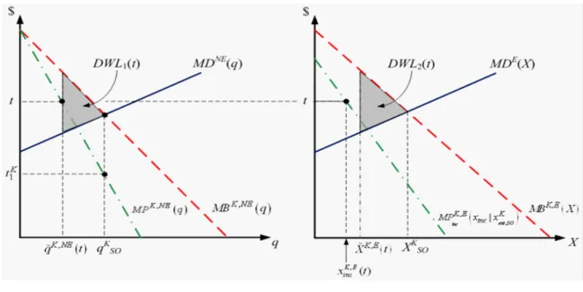
M BK;N E(q) M DN E(q) dq, where output q~K;N E(t) solves M PincK;N E(q) =t, i.e., q~K;N E(t) is the monopoly pro…t-maximizing output for a given fee t. Figure 1a below illustrates the …rst-period welfare loss of setting a fee t that di¤ers from the socially optimal fee tK1 . In particular, …gure 1a depicts the case where t > tK1 , leading to a monopoly output q~K;N E(t) that lies below the socially optimal outputqSOK .14
1 2
Intuitively, this implies that the importance that the social planner assigns to consumer surplus and environmental damage must be relatively close. If instead, the environmental damage is extremely low (high) and the weight on consumer surplus is high (low), the regulator would choose to not reduce output levels setting a zero fee (reduce output to zero by setting a high fee, respectively).
1 3
Since we analyze social welfare across two time periods, the example assumes no discounting of future payo¤s.
1 4In order to allow for the case wheret < tK
1, expression (6) considers the absolute value of the deadweight loss of feet.
Figure 1a Figure 1b
Similarly, the deadweight loss associated with taxtin the second period is given byDW L2(t)
Z XSOK;E
e
XK;E(t)
M BK;E(X) M DE(X) dX, where XeK;E(t) = xK;Einc (t) +xK;Eent (t) and output xK;Ej (t)
solves M PjK;E xjjxK;Ek;SO = t for all …rm j, i.e., xK;Ej (t) represents …rm j’s pro…t-maximizing
output for a given feetafter entry. Deadweight lossDW L2(t)is depicted in …gure 1b. Speci…cally,
the constant fee t maps into M PincK;E( ), inducing the incumbent to produce xK;Einc (t). However, DW L2(t) is calculated from aggregate duopoly outputXeK;E(t).
Entry deterrence. In the context of an in‡exible environmental policy, the regulator can commit to a relatively high feetthat deters entry, i.e., a fee that lowers the entrant’s duopoly pro…ts below his …xed entry cost F. Let SWH;N E t denote overall social welfare when the incumbent’s costs are high, and the regulator commits to a su¢ ciently high feetthat deters entry.15 Intuitively, the welfare cost of deterring entry arises from substantially reducing the incumbent’s monopoly output across both periods, thereby decreasing consumer surplus and pro…ts, whereas its welfare bene…t emerges from the reduction in pollution and the savings in entry costs.
Example. Continuing with our example, and considering R = 1 and = 1, the optimal tax
t that the regulator chooses across both periods is tL;N E = (2d 1)xK;N ESO when the incumbent’s costs are low and therefore entry does not occur. In this case, the welfare-maximizing emission fee 1 5Note that the use of high fees can only serve to deter entry if environmental policy is in‡exible along time. If,
in contrast, fees can be modi…ed after the …rst period, entry cannot be credibly deterred. In addition, when the incumbent’s costs are low, entry does not occur, and the regulator does not need to commit to a high emission feet in order to deter entry. We hence restrict our analysis to the regulation of the high-cost incumbent.
coincides with that under a ‡exible policy,tL;N E =tL1 =tL;N E2 . The regulator has no incentive to revise the environmental policy because a monopoly is regulated at each stage. In contrast, when the incumbent’s costs are high, entry occurs and the optimal tax is a weighted average of …rst- and second-period taxes,16 tH;E = 259tH1 + 1625tH;E2 , and thus tH1 < tH;E < tH;E2 . Finally, note that the regulator can deter entry by setting a feetthat solves H;Eent (t) =F, i.e.,t= 1 cH
inc 3
p
F, which decreases as entry becomes more costly, thus facilitating entry deterrence; and it is positive for all F < F (1 cHinc)2
9 . This fee yields an overall social welfare ofSW
H;N E t = 3
p
F[4 (3+6d)pF 4cH inc]
4 ,
whereas the social welfare from setting an in‡exible feetH;E that attracts entry isSWH;E tH;E =
49 49(2 cH inc)cHinc
50(1+2d) F.
The following lemma examines the regulator’s incentives to set entry-deterring fees where the given institutional setting is in‡exible.
Lemma 1. Under an in‡exible policy regime, the social welfare from committing to an
entry-deterring fee t,SWH;N E t , exceeds that from setting a fee tH;E that attracts entry,SWH;E tH;E ,
if and only if F > FInf lex(d). In addition, cuto¤ FInf lex(d) satis…es FInf lex(d)< H;Eent tH;E .
The …gure below represents cuto¤ FInf lex(d) for the case where cHinc = 14. Intuitively, when entry costs are higher thanFInf lex(d), entry can be deterred by committing to a low feet, thereby
incurring a small welfare loss.17 In addition, as entry becomes more costly (higher F), entry-deterrence can be sustained under a larger set of environmental damages, d. For (F; d)-pairs below FInf lex(d), in contrast, entry deterrence becomes more di¢ cult since fee t is high, thereby
producing a large welfare loss, without entailing a substantial environmental bene…t given that d is small. Hence, allowing entry is socially optimal.
1 6It is straightforward to show that this fee generates strictly positive production levels for both incumbent and
entrant across periods. In addition, as the R!0, the weight ontH1 increases and that ontH;E2 decreases. Intuitively, the social planner assigns no value to the future deadweight loss and therefore selects a fee that minimizes deadweight loss in the …rst-period game.
1 7Note that the entry-deterring feetis strictly positive since cuto¤F lies above H;E ent t
H;E
2 for all parameter values; as shown in the proof of Lemma 1.
Figure 2. Cuto¤FInf lex(d)and H;Eent tH;E2 .
Blockaded entry. For comparison purposes, …gure 2 also includes the threshold under which entry costs are su¢ ciently high, making entry unpro…table under a ‡exible policytH;E2 , i.e., for all F > H;Eent tH;E2 and entry is blockaded. Importantly, note that cuto¤FInf lex(d) lies below the
threshold for which entry is blockaded, allowing the regulator to practice entry deterrence if entry costs are intermediate. In our parametric example, for instance, the threshold for which entry is blockaded isF > H;Eent tH;E2 (1 c
H inc)
2
4(1+2d)2 > FInf lex(d).
5
Welfare comparisons
We can now examine the …rst period of the game, where the regulator chooses between a ‡exible and an in‡exible policy. Furthermore, if an in‡exible policy is selected, the regulator needs to decide whether to set a su¢ ciently high feetthat deters entry. As described above, when the incumbent’s costs are low, entry does not occur, and optimal emission fees coincide in both policy regimes, yielding similar welfare. When the incumbent’s costs are high, however, emission fees not only di¤er in both policy settings, but also allow for the use of the emission fee as an entry-deterrence device.
Let us …nally introduce additional notation. Let FF lex(d) represent the entry cost that makes the regulator indi¤erent between selecting an in‡exible fee that deters entry, yieldingSWH;N E t , and setting a ‡exible policy, resulting in an overall welfare of SWH;E tH1 ; tH;E2 . In our above parametric example, cuto¤FF lex(d) lies above cuto¤FInf lex(d) under all feasible values of d; as depicted in …gure 3.18 Intuitively, a regulator is less willing to bear the welfare loss of deterring entry
1 8
when he chooses a ‡exible policy than when he is already committed to a constant environmental policy. The following proposition summarizes the regulator’s policy choice in the subgame-perfect equilibrium of the game. For presentation purposes, let region I represent entry costs where F < FInf lex(d) (see …gure 3), region II the case in which FInf lex(d)< F < FF lex(d), region III denote the case whereFF lex(d)< F < H;E
ent t H;E
2 , and in region IV entry costs satisfyF >
H;E ent t
H;E
2 .
Figure 3. Cuto¤sFF lex(d),FInf lex(d)and H;Eent tH;E2 :
Proposition 1. In equilibrium, the regulator selects:
1. A ‡exible policy that attracts entry both in region I and II, since social welfare satis…es
SWH;E tH1 ; tH;E2 > SWH;E tH;E > SWH;N E t and SWH;E tH1 ; tH;E2 > SWH;N E t >
SWH;E tH;E , respectively;
2. An in‡exible policy tthat deters entry in region III, since social welfare satis…esSWH;N E t >
SWH;E tH1 ; tH;E2 > SWH;E tH;E ; and
3. A ‡exible policy that blockades entry in region IV.
The regulator’s decision can therefore be divided into four regions. When entry costs are su¢ -ciently low, F < FInf lex(d), he prefers to set a ‡exible policy, since it yields a larger social welfare than an in‡exible policy. This case is graphically represented in region I of …gure 3. Intuitively,
entry can only be deterred by committing to a relatively stringent fee t, which reduces the incum-bent’s monopoly output during both periods, thus signi…cantly decreasing consumer and producer surplus. Furthermore, deterring entry entails a small bene…t since the environmental damage from pollution, d, is relatively small in this region. As a consequence, the welfare loss from setting t o¤sets its associated environmental bene…ts, and a ‡exible environmental policy is welfare supe-rior. A similar argument holds when entry costs are moderately low,FInf lex(d)< F < FF lex(d)in region II, where ‡exible policies also yield a larger welfare.19 When entry costs are relatively high, however, social welfare can be maximized by deterring entry. In region III, entry can be deterred by imposing a relatively lowt, thereby incurring small welfare losses from reducing the incumbent’s monopoly output. In addition, such output reduction entails signi…cant environmental bene…ts, provided thatdis relatively high, which ultimately increases overall welfare. Our results hence sug-gest that governments maintain ‡exible environmental policies in industries with low entry costs and small environmental damages — which facilitates entry— but commit to relatively high fees otherwise, thus hindering entry.
Finally, the region under which entry deterrence becomes socially optimal (region III) shrinks in the entrant’s costs. In particular, an increase in cent produces a downward shift in the entrant’s
duopoly pro…ts, H;Eent tH;E2 , reducing the distance H;Eent tH;E2 FF lex(d). Intuitively, when the
entrant is more ine¢ cient, its pro…ts upon entry decrease, making him less attracted to the market, and hence the regulator’s task of deterring entry becomes less necessary.
Incumbent pro…ts. From a policy perspective, the setting of stringent environmental policies is commonly regarded as a tool governments may use to deter entry and promote the pro…ts of domestic monopolies. The next corollary shows that this is not necessarily true in our model.
Corollary 1. The pro…ts of the high-cost incumbent are larger when the regulator sets an
entry-deterring fee t than under any other policy if and only if F > FP rof its(d), where FP rof its(d)
1274(1 cHinc)2 5625(1+2d)2 .
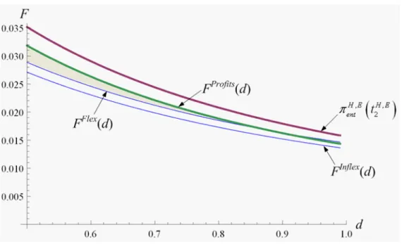
In particular, feethelps the incumbent maintain her monopoly power, but signi…cantly reduces her output and pro…ts during both periods. As a consequence, the high-cost incumbent prefers that the regulator deters entry only when feet, and thus the pro…t loss that she must bear, is relatively small. This speci…cally occurs when entry is easy to deter, i.e., entry costs are relatively high. In particular, …gure 4 superimposes cuto¤FP rof its(d) on …gure 3, identifying the region where the incumbent prefers to bear a stringent fee t in order to deter entry, when F > FP rof its(d), or she prefers entry otherwise (shaded area).
1 9
The di¤erence with region I arises o¤-the-equilibrium path since, if the regulator commits to a constant environ-mental policy, social welfare is now larger by setting an entry-deterrence feetthan by commiting to feetH;E.
Figure 4. Pro…ts in the entry-deterring equilibrium.
From Proposition 1, the regulator selects an entry-deterring fee t when FF lex(d) < F <
H;E ent t
H;E
2 . Therefore, the regulator and incumbent’s preferences are aligned when entry costs
lie in the region above cuto¤FP rof its(d)and below H;Eent tH;E2 in …gure 4. The shaded area rep-resents, in contrast, parameter combinations under which deterring entry is sequentially rational for the regulator, i.e., F > FF lex(d), but such practice imposes a signi…cant pro…t loss on the incumbent, thereby diminishing her overall pro…ts. In summary, when entry costs are su¢ ciently high, F > FP rof its(d), both the regulator and the high-cost incumbent are willing to bear the cost of a stringent environmental policy in order to deter entry. In contrast, when entry costs are relatively low (in the shaded area), entry-deterrence becomes costly, implying that the incumbent prefers entry rather than bearing the large cost of the strict fee t that avoids entry, whereas the regulator still …nds entry-deterrence socially optimal.
6
Conclusions
Our paper examines under which conditions governments strategically commit to relatively strin-gent environmental policies in order to maximize social welfare. We show that entry deterrence becomes socially optimal when its associated welfare loss, due to committing to a stringent fee across time, is smaller than its welfare gain, which arises from an improved environmental quality. Otherwise, the regulator optimally chooses a ‡exible environmental policy which cannot credibly deter entry. In addition, we demonstrate that the incentives of the social planner and incumbent are not necessarily aligned regarding entry deterrence. In particular, under certain conditions the
regulator …nds socially optimal to commit to an in‡exible policy that deters entry whereas the incumbent would actually prefer a ‡exible policy that attracts entry.
The paper assumes that the entrant observes the incumbent’s costs. In di¤erent settings, how-ever, the entrant might not have access to this information, thereby inferring the incumbent’s type after observing not only the incumbent’s production decision but also the regulator’s environmental policy. In such context, environmental regulation can facilitate or hinder the incumbent’s informa-tion transmission. In addiinforma-tion, we consider a single incumbent, which could be modi…ed to allow for multiple incumbents; as in Gilbert and Vives (1986). Unlike their work, however, free-riding incentives are absent in our model since the incumbents’output choices do not condition entry de-cisions. Finally, our paper can be extended to the analysis of non-polluting goods. In this case, the regulator would not impose taxes but rather provide subsidies in order to induce …rms to produce the socially optimal output.
7
Appendix
7.1 Appendix 1
Let us analyze the existence of socially optimal output and emission fees under complete informa-tion.
Second period, No entry. The socially optimal output under monopoly xK;N ESO solves M BK;N E(x) =M DN E(x), where M BK;N E(x) @[ CS+ K;N E inc ] @x = (1 )p 0(x)x+p(x) cK inc
and M DN E(x) d0(x). Socially optimal output under monopoly xK;N ESO exists if M BK;N E(0)> M DN E(0), which holds since p(0) cKinc> d0(0). The emission fee that induces the monopolist to produce xK;N ESO is tK;N E2 = M PincK;N E xK;N ESO , where M PincK;N E(xinc) @
K;N E inc (xinc)
@xinc . Note that
tK;N E2 is decreasing in costs. In particular, an increase in costs shifts the M PincK;N E(xinc) function
downwards, decreasing the value of xK;N ESO that solves M BK;N E(x) = M DN E(x). Given that M DN E(x) is una¤ected by the change in costs and it is increasing inx, the optimal value oftK;N E
2
decreases.
Second period, Entry. The socially optimal aggregate output under duopoly XSOK;E solves M BK;E(X) =M DE(X), where
M BK;E(X) (1 )p0(X)X+p(X) cKinc
and M DE(X) d0(X) whereX =xinc+xent. In addition, M BK;E(X) is decreasing in X since
its slope is (2 )p0(X) given linear demand, which is negative since 1, and M DE(X) is increasing inXsince its slope isd00(X)>0. Optimal aggregate output under duopolyXK;E
ifM BK;E(0)> M DE(0), which holds sincep(0) cKinc> d0(0). The emission feetK;E2 that induces the aggregate output XSOK;E is tK;E2 = M PjK;E xK;Ej;SOjxK;Ek;SO for all j = finc; entg and k 6= j, where M PjK;E xjjxK;Ek;SO
@ K;Ej (xjjxK;Ek;SO)
@xj for all …rm j 6=k. Note thatt
K;E
2 is decreasing in the
incumbent’s costs, i.e., tL;E2 > tH;E2 . In particular, an increase in the incumbent’s costs decreases XSOK;E since both …rms’best response functions have a slope larger than 1. That is,
@xent(xinc) @xinc = @2 K;d ent @xent@xinc @2 K;d ent @x2 ent = p 0+p00xent 2p0+p00xent > 1
wherep p(X) andp00= 0 given that demand is linear. Given thatM DE(X)is una¤ected by the change in costs and it is increasing in X, the optimal value oftK;E2 decreases.
First period.The socially optimal output under …rst-period monopolyqKSOsolvesM BK;N E(q) =
M DN E(q), where
M BK;N E(q) (1 )p0(q)q+p(q) cKinc
and M DN E(q) d0(q). By a similar argument as fortK;E2 emission feetK1 exists and is decreasing in costs.
7.2 Proof of Lemma 1
Under an in‡exible policy regime, the social welfare from setting a constant entry-deterring fee t= 1 cH inc 3 p F is SWH;N E(t) = 3pFh4 (3 + 6d)pF 4cHinci 4
where the high-cost incumbent produces according to the monopoly output functionqH(t) = 1 cHinc
2
during both periods. If, in contrast, the regulator selects a constant feetH;E, entry ensues, yielding an overall social welfare of
SWH;E(tH;E) = 49 49(2 c
H inc)cHinc
50(1 + 2d) F
Hence, the regulator prefers to deter entry, i.e., SWH;N E(t) > SWH;E(tH;E), if F > FInf lex(d), where
FInf lex(d) 1310 + 8d(557 + 459d) 60
p
2(1 cHinc)2G 2(1 + 2d)(655 + 918d)(2 cHinc)cHinc
25(5 + 28d+ 36d2)
and G (1 + 2d)3(205 + 18d) 1
2. First, note that cuto¤FInf lex(d)is decreasing in dfor all costs
cHinc2(0;1). Second, cuto¤FInf lex(d) lies below F (1 c
H inc)
2
d2 12;1 . In particular, the highest point of cuto¤FInf lex(d),FInf lex 12 , is
557 30(1 cHinc)2p214 557(2 cHinc)cHinc
2450
which is lower than F (1 c
H inc)
2
9 , which is constant in d, for all costs c
H
inc 2(0;1). Third, cuto¤
FInf lex(d) also lies below the entrant’s duopoly pro…ts under the ‡exible fee tH;E2 , H;Eent (tH;E2 ). Speci…cally, H;Eent (tH;E2 ) = (1 c
H inc)
2
4(1+2d)2 is decreasing ind, reaching its highest value atd= 12, (1 cH
inc)
2 16 ,
which lies above FInf lex 12 ; and reaches its lowest value at d = 1, (1 c
H inc)
2
36 , which also lies
above FInf lex(1). Fourth, note that the entrant’s duopoly pro…ts under the in‡exible fee tH;E,
H;E ent (tH;E) = 196(1 cH inc) 625(1+2d) , satisfy H;E ent (tH;E) > H;E ent (t H;E 2 ) since tH;E < t H;E
2 , i.e., tH;E is less
stringent than tH;E2 . Therefore, ifFInf lex(d) satis…esFInf lex(d)< H;E ent (t
H;E
2 ), then FInf lex(d)< H;Eent (tH;E2 )< H;Eent (tH;E).
Finally, note that pro…ts H;Eent (tH;E)lie below cuto¤F . Indeed, H;Eent (tH;E)reaches its highest point at d = 12, 49(1 c
H inc)
2
625 , which is lower than cuto¤F . SinceF is constant in d, then F >
H;E
ent (tH;E) under all parameter values.
7.3 Proof of Proposition 1
Second period. Under no entry, the K-type incumbent solves
max
xinc
(1 xinc)xinc cKinc+t xinc
which is maximized at xK;N Einc (t) = 1 (c
K inc+t)
2 for any fee t set by the regulator (notice that this
allows for ‡exible and in‡exible policies). Similarly, under entry, the incumbent solves
max
xinc
(1 xinc xent)xinc cKinc+t xinc.
whereas the entrant solves a similar problem, where his marginal production costs are high. In this subgame, the K-type incumbent selects a duopoly output of xK;Einc (t) = 1 2(c
K
inc+t)+(cent+t)
3
and the entrant chooses xK;Eent (t) = 1 2(cent+t)+(c
K inc+t)
3 . In this context, the socially optimal output XSOK that solves M BK;N E(x) = M DN E(x), which implies (1 )x+ (1 x) cKinc = 2dx, is XSOK = 1 cKinc 2+2d , which is positive ifd2 h 2; 1+ 2 i
. Under no entry, the regulator can induceXSOK by setting a second-period fee that satis…estK;N E2 =M PincK;N E(XSOK;N E), that istK;N E2 = (2d )XSOK . Similarly, under entry, the social planner seeks to induce the same socially optimal output XSOK . This implies that, in order to …nd fee tK;E2 and individual output levelsxK;Ej;SO and xK;Ek;SO, the social planner must simultaneously solve xK;Ej;SO +xK;Ek;SO = XSOK;E and tK;E2 = M PjK;E xK;Ej;SOjxK;Ek;SO for both …rms j =finc; entg. In the context of our example, this implies tH;E2 = (1 + 4d 2 )X
H;E SO
when the incumbent’s costs are high. Note that this yields pro…ts of H;Eent tH;E2 (1 c
H inc)
2 4(1+2d)2 for
the entrant, implying that entry is blockaded when the …xed entry costs, F, are su¢ ciently high, i.e., F > (1 c
H inc)
2
4(1+2d)2 . When the incumbent’s costs are low, the regulator sets a second-period fee
tL;E2 = A(1 cHinc) B(1 cLinc)
2A , where A 2 + 2d and B 1 2d+ . This fee and the resulting
duopoly output are positive as long the di¤erence between the incumbent’s and entrant’s cost is not too large, i.e.,cLinc< cHinc< 1+DcLinc
A , where D 1 + 2d .
First period. Since the incumbent operates as a monopolist in the …rst-period game, she chooses output function qK(t) = 1 (c
K inc+t)
2 for any fee t. Given this output function, under a
‡exible environmental policy the regulator sets a …rst-period fee tK1 that solves tK1 =M PincK(qKSO)
where qSOK denotes the socially optimal output qKSO = 1 cKinc
2+2d , i.e., fee tK1 = (2d )qSOK . Under
an in‡exible policy, the regulator sets a feetL;N E when the incumbent’s costs are low (and thus he anticipates no entry to ensue in the second period) where tL;N E coincides with …rst- and second-period fees under no entry, i.e., tL;N E =tL1 =tL;N E2 . In contrast, when the incumbent’s costs are high, the regulator anticipates entry in the following period, thus setting a feetH;E that minimizes the deadweight loss as described in expression (6) in the text, i.e., tH;E = 259 tH1 + 1625tH;E2 where tH
1 < tH;E < t
H;E
2 . In this setting, however, the regulator can choose to commit to an entry-deterring
feet such that H;Eent (t)< F for all t > t. In particular, given that entH;E(t) = 19(1 cent t)2, the
fee tthat solves H;Eent t = F is t = 1 cHinc 3pF. This fee t is positive for all F < F , where F (1 c
H inc)
2 9 .
Finally, the regulator chooses whether to maintain a ‡exible policy across periods or to commit to a given emission fee and, if so, whether to allow or deter entry. When the incumbent’s costs are low, entry does not occur, and thus the regulator maximizes social welfare by selecting a ‡exible policy. When the incumbent’s costs are high, however, entry ensues as long as the constant fee t does not exceedt. The overall social welfare that the regulator obtains from setting ‡exible emission fees tH 1 and t H;E 2 is SWH;E tH1 ; t H;E 2 = 1 (2 cH inc)cHinc
1+2d F, that of committing to a constant fee
tH;E that allows entry is SWH;E tH;E = 49 49(2 cHinc)cHinc
50(1+2d) F, and that of committing to an
entry-deterring fee t is SWH;N E t = 3 p
F[4 (3+6d)pF 4cHinc]
4 . It is straightforward to show that SWH;E tH
1 ; t
H;E
2 > SWH;E t when F < FF lex(d), where FF lex(d) 48(1 c
H
inc)2(1 + 2d)3=2 R
(5 + 28d+ 36d2)2
and 52 + 16d(11 + 9d) and R 4(1 + 2d)(13 + 18d)(2 cHinc)cHinc. In addition,SWH;N E t > SWH;E tH;E when F > FInf lex(d), as described in Lemma 1, and FInf lex(d) < FF lex(d). This implies that when F < FInf lex(d), social welfare satis…es SWH;E tH1 ; tH;E2 > SWH;E tH;E > SWH;N E t , and the regulator sets a ‡exible policy; when FInf lex(d) < F < FF lex(d), social welfare satis…es SWH;E tH1 ; tH;E2 > SWH;N E t > SWH;E tH;E , and the regulator also sets a ‡exible policy; when FF lex(d) < F < entH;E tH;E2 , social welfare satis…es SWH;N E t >
SWH;E tH1 ; tH;E2 > SWH;E tH;E , and the regulator commits to an in‡exible fee t that de-ters entry; and when F > H;Eent tH;E2 , entry is blockaded and the regulator selects a ‡exible environmental policy.
7.4 Proof of Corollary 1
The pro…ts of the high-cost incumbent when the regulator sets an entry-deterring feet= 1 cHinc
3pF are 94F during both the …rst and second period, where the high-cost incumbent produces according to the monopoly output functionqH(t) = 1 cHinc
2 during both periods, yielding an overall
pro…t of 184F.
If the regulator chooses a ‡exible policy regime, with equilibrium fees tH1 and tH;E2 for the …rst and second-period, respectively, the high-cost incumbent’s pro…ts become (1 cHinc)2
(1+2d)2 in the …rst
period and (1 cHinc)2
4(1+2d)2 in the second period (after entry ensues). Hence, overall pro…ts are 5(1 cH
inc)2
4(1+2d)2 .
Therefore, pro…ts under the entry-deterring fee tare larger than under the ‡exible fees tH1 ; tH;E2 for all F > FP rof its;F lex(d) whereFP rof its;F lex(d) 5(1 cHinc)2
18(1+2d)2.
If the regulator selects an in‡exible policy regime, with equilibrium fee tH;E, the high-cost incumbent’s pro…ts become 441(1 cHinc)2
625(1+2d)2 in the …rst period and
196(1 cH inc)2
625(1+2d)2 in the second period
(after entry ensues). Hence, overall pro…ts are (9+4 )(3+4 )2(1 cHinc)2
(9+16 )2(2+2d )2 , or
637(1 cH inc)2
625(1+2d)2 when = = 1.
Therefore, pro…ts under the entry-deterring fee t are larger than under the in‡exible fee tH;E for all F > FP rof its;Inf lex(d) whereFP rof its;Inf lex(d) 1274(1 cHinc)
2 5625(1+2d)2 .
In addition, note that cuto¤FP rof its;Inf lex(d)> FP rof its;F lex(d), since the di¤erence FP rof its;Inf lex(d) FP rof its;F lex(d) = 98(1 c
H inc)2
625(1 + 2d)2
is positive under all parameter values. Furthermore, H;Eent (tH;E) > FP rof its;Inf lex(d) since the di¤erence
H;E
ent (tH;E) FP rof its;Inf lex(d) =
98(1 cHinc)2 1125(1 + 2d)2
is positive under all parameter values. Therefore, H;Eent (tH;E)> FP rof its;Inf lex(d)> FP rof its;F lex(d). Hence, the region of parameter values under which the regulator prefers to practice entry deterrence but the high-cost incumbent does not occurs whenF < FP rof its;Inf lex(d). Otherwise, both agents prefer the entry-deterring feet. Therefore, only cuto¤FP rof its;Inf lex(d)is binding, and we denote FP rof its;Inf lex(d) asFP rof its(d).
References
[1] Alvarez, F., P.J. Kehoe and P.A. Neumeyer. (2004). “The time consistency of optimal
[2] Bain, J.(1956) Barriers to New Competition, Cambridge, Harvard University Press.
[3] Barro, R. and D. Gordon(1983). “A positive theory of monetary policy in a natural rate model.” Journal of Political Economy 91, pp. 589-610.
[4] Benhabib, J.,A. Rustichini, and A. Velasco(2001). “Public spending and optimal taxes
without commitment.” Review of Economic Design 6, pp. 371-396.
[5] Brock, W. and D. Evans (1985) “The Economics of Regulatory Tiering.” RAND Journal
of Economics, 16(3), pp. 398-409.
[6] Chamley, C.(1986). “Optimal taxation of capital income in general equilibrium with in…nite lives.” Econometrica 54, pp. 607-22.
[7] Chang, R. (1998). “Credible monetary policy in an in…nite horizon model: Recursive ap-proach.” Journal of Economic Theory 81, pp. 431-461.
[8] Dean, T. and R. Brown(1995) “Pollution regulation as a barrier to new …rm entry: Initial evidence and implications for further research.” Academy of Management Journal, 38(1), pp. 288–303.
[9] Dean, T., R. Brown and V. Stango(2000) “Environmental Regulation as a Barrier to the
Formation of Small Manufacturing Establishments: A Longitudinal Examination.” Journal of Environmental Economics and Management, 40(1), pp. 56-75.
[10] Dixit, A. (1980) “The role of investment in entry-deterrence.” Economic Journal 90, pp. 95-106.
[11] Dixit, A. and L. Lambertini(2003) “Interactions of Commitment and Discretion in
Mon-etary and Fiscal Policies.” American Economic Review 93(5), pp. 1522-42.
[12] Fudenberg, D. and J. Tirole(1984) “The fat-cat e¤ect, the puppy-dog ploy, and the lean and hungry look.” American Economic Review, 74(2), pp. 361–66.
[13] Gilbert, R. and X. Vives(1986) “Entry deterrence and the free-rider problem.”Review of Economic Studies 172, pp. 71-83.
[14] Helland, E. and M. Matsuno(2003) “Pollution Abatement as a Barrier to Entry.”Journal
of Regulatory Economics, 24(2), pp. 243-259.
[15] Ko, I., H.E. Lapan, and T. Sandler (1992) “Controlling stock externalities: Flexible
versus in‡exible pigouvian corrections.” European Economic Review 36. pp. 1263-1276. [16] Kydland, F. and E. Prescott(1977) “Rules rather than discretion: The inconsistency of
[17] Kovenoch, D. and S. Roy (2005) “Free-riding in non-cooperative entry deterrence with di¤erentiated products.” Southern Economic Journal 72, pp. 119-137.
[18] Monty, R. L.(1991) “Beyond environmental compliance: Business strategies for competitive advantage.” Environmental Finance, 11(1), pp. 3–11.
[19] OECD (2006) “Environmental Regulation and Competition.” OECD Competition Policy Rountables. Directorate for Financial and Enterprise A¤airs, Competition Committee. [20] Ryan, S. (2011) “The Costs of Environmental Regulation in a Concentrated
Industry.”forth-coming in Econometrica.
[21] Spence, M. (1977) “Entry, capacity, investment and oligopolistic pricing.” Bell Journal of Economics 10, pp. 1-19.
[22] Stavins, R. (2005) “The E¤ects of Vintage-Di¤erentiation Environmental Regulation.” Dis-cussion paper, Resources for the Future, Washington, D.C.
[23] Sylos-Labini, P. (1962) Oligopoly and Technical Progress, Cambridge, Harvard University Press.
[24] Ungson, G., C. James and B. Spicer (1985) “The E¤ects of Government Regulatory
Agencies on Organizations in High Technology and Woods Products Industries.”Academy of Management Journal, 28 (2), pp. 426-445.
[25] Waldman, M.(1987) “Noncooperative entry deterrence, uncertainty and the free-rider prob-lem.” Review of Economic Studies 54, pp. 301-10.
[26] Ware, R.(1984) “Sunk Costs and Strategic Commitment: A Proposed Three-Stage