Learning to Detect Drowsiness in Drivers
Antti Takalahti
Master’s Thesis
UNIVERSITY OF HELSINKI Department of Computer Science
Faculty of Science Department of Computer Science
Antti Takalahti
Learning to Detect Drowsiness in Drivers
Computer Science
Master’s Thesis April 19, 2016 61
Drowsiness, Machine learning, Driving
Supervised machine learning consists of inferring a function from labelled examples. The examples used in this study are twenty second stretches of driving data and the labels are binary values of visually scored drowsiness.The ultimate goal is to predict future driving performance by looking only at the steering wheel angle and the position of the accelerator pedal over time.
Chapter two explains what drowsiness is, how tools such as electroencephalogram and electrooculogram reveal drowsiness, and what other tools have been used to study drowsiness.
Chapter three shows how a driver’s drowsiness can be detected, and what the psychological aspects relevant to driving performance are. Some currently used methods are also described.
Chapter four shows how the Karolinska drowsiness score is derived from electroencephalo-gram and electrooculoelectroencephalo-gram, and how this score is used to train the nearest neighbour classifier to detect drowsiness from individual segments of driving data and further to predict driving performance.
Tiedekunta — Fakultet — Faculty Laitos — Institution — Department
Tekijä — Författare — Author
Työn nimi — Arbetets titel — Title
Oppiaine — Läroämne — Subject
Työn laji — Arbetets art — Level Aika — Datum — Month and year Sivumäärä — Sidoantal — Number of pages
Tiivistelmä — Referat — Abstract
Avainsanat — Nyckelord — Keywords
Contents
1 Introduction 1
2 Using Biomarkers to Measure Drowsiness 2
2.1 Drowsiness, Sleepiness, Tiredness, and Fatigue . . . 2
2.2 Biomarkers for Human Drowsiness . . . 7
2.3 Statistical Methods in Drowsiness Detection . . . 10
3 Evaluating the Driving Performance of the Driver 16 3.1 Psychological Issues Related to Driving Performance . . . 16
3.2 Biomarkers for Driver Drowsiness . . . 21
3.3 Existing Solutions for Detecting Drowsiness in Drivers . . . . 25
4 Learning to Predict Sleepiness on the Basis of Car Data 30 4.1 Data Source and Measurements . . . 31
4.2 Summary Statistics Used to Train a Classifier . . . 35
4.3 Training the classifier . . . 38
4.4 Results . . . 41 5 Conclusions 49 5.1 Discussion . . . 50 5.2 Summary of Contributions . . . 52 5.3 Future Research . . . 53 References 54
1
Introduction
There are more than a billion cars on the roads worldwide, and falling asleep while driving is common [65]. In a study conducted in the United States by the Centers for Disease Control and Prevention, one in every twenty-five adult respondents reported having fallen asleep while driving during the last thirty days [27]. In another study, done in Finland by the Finnish Road Safety Council Liikenneturva, it was shown that a quarter of the population had at least once fallen asleep while driving [49].
The aim of my study is to show how a driver´s drowsiness can be detected using common machine learning methods. I will do this by applying three frequently used methods to a data set collected in a study made in Sweden. In that study, drowsiness was measured in eighteen drivers as they drove for approximately ninety minutes first during daytime and then during the night. The drivers’ level of drowsiness was measured with the use of an eye camera, by measuring the electrical activity of the brain and by recording the eye movement.
Machine learning has been previously used to detect sleep from the electrical activity of the brain and in how drivers drive in a simulator by recording how they negotiated curves and then using machine learning to learn the difference in alert and drowsy driving. Being tired changes the behaviour of the driver. While the exact effects of drowsiness are difficult to define, one can use machine learning as long as one has some form of biomarker for the level of drowsiness.
Machine learning has huge potential as the race to develop autonomously driving cars rages on, producing vast amounts of data each day. Soon we will have similar data at our use as airline accident investigators, with cars carefully recording the moments leading up to the accident. Driving performance goals like lane position, distance to other cars and flow of traffic are perfectly suited for machine learning algorithms and learning is a perfect tool for creating solutions to these problems.
I will first look at how drowsiness affects people in general and how it can be measured. I will then take a look at how drowsiness can be detected in drivers and show how machine learning can be used as a tool for drowsiness detection. Finally, I will present my own study, where I try to predict which drivers fail to complete their night time drive by learning from a human
scored measure of drowsiness and applying that knowledge to the steering wheel angle, vehicle speed, and accelerator pedal position.
2
Using Biomarkers to Measure Drowsiness
2.1 Drowsiness, Sleepiness, Tiredness, and Fatigue
In this study, the terms drowsiness, sleepiness, tiredness, and fatigue are used as synonyms. This is of course a gross generalisation, but serves the purposes of this study. The main aim of the study is not to distinguish between these different phenomena, but rather on studying their common effects and to show how they can be measured.
Sleepiness research is usually about problems related to sleep – the effects of drugs and illnesses. A condition where person feels compelled to nap even after a normal night’s sleep. Tiredness refers to a condition that causes continuous feeling to tiredness or fatigue. This is generally more about the lack of energy and not about feeling the need to sleep. Fatigue research studies how physical exercise, emotional stress and boredom cause a feeling of tiredness. Drowsiness research is in general terms about boredom and monotonous tasks and their effects of person.
Currently the best way to measure the level of drowsiness of a human being is the multiple sleep latency test [16]. The multiple sleep latency test combines the use of sleep diaries, polysomnography done during one night, and a test where the testee goes into a dark, quiet, and temperature-controlled room to lie down for twenty minutes at a time several times during one day. The aim of the multiple sleep latency test is to measure the sleep latency, or the time it takes for the person to fall asleep. The tests are started 90–180 minutes after the testee has woken up, and they are done with two hour intervals. A minimum of four tests is required for a full analysis.
Various signals are recorded during this test. The most interesting ones are the electroencephalogram (EEG), electrooculogram, and electromyogram. This is the trio that is most often used to measure drowsiness in all kinds of experiments. EEG measures the electrical activity of the brain using electrodes placed on the testee’s scalp. Electrooculogram records the move-ment of the eyes and is used to study the deeper stages of sleep [14]. The electromyogram records the electrical activity of skeletal muscles.
Rhythm Frequency (Hz) Delta below 3.5 Theta 4-7.5 Alpha 8-13 Beta 14-30 Gamma above 30
Table 1: EEG rhytms EEG measures the electrical activity of the
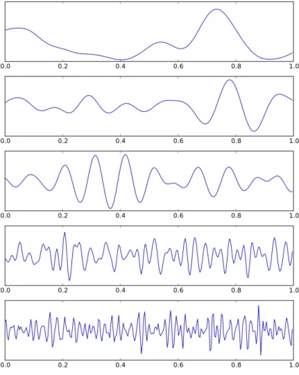
brain. Multiple electrodes are placed on the testee’s scalp to detect neural oscillations. Hans Berger discovered the alpha rhythm in 1929 [10] and since then many more rhythms have been found [56]. The main ones are shown in Table 1 and in Fig. 1. The typical amplitude of these waves ranges from 0 to 200 µV.
The alpha rhythm is the classical pattern
that emerges when a subject is awake, relaxed, and has their eyes closed. Any kind of movement or visual stimulus as well as concentrating hard distorts the alpha rhythm. There are individual differences, and it is important to start off with a controlled period of relaxation with eyes closed. Niedermayer and da Silva report that the voltage range for alpha rhythm is usually between 0 and 50µV, and that values of above 100µV are uncommon in adults.
A subject’s level of alertness fluctuates in the process of falling asleep. The criterion for ’being asleep’ in the multiple sleep latency test [16] is that more than a half of a thirty second time-frame should consist of sleep, which in turn is defined as either the presence of delta and theta waves, or as an activity in higher frequency with a lower amplitude than what is measured from delta and theta waves [61]. Niedermeyer calls this the alpha dropout [56] and considers it a first sign of drowsiness.
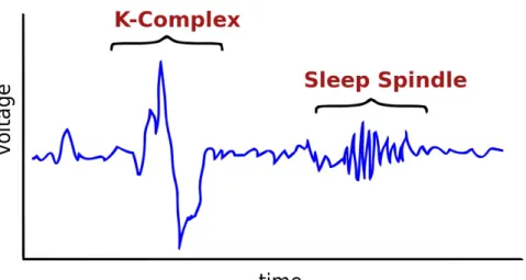
Another sign of early sleep is the presence of slow rolling eye movements [9]. Typically, the frequency of these movements will vary in the range of 0.25Hz to 0.5Hz, and they are usually detected simultaneously with alpha dropout. They show up in EEG as well as in the electrooculogram. Multiple signals help in detecting the source for various artefacts seen in EEG data. Electromyogram detects chewing, swallowing, and the movement of the tongue. In some cases, heartbeat can also show up in the EEG. This rhythm can be filtered out by combining the data with the electrocardiogram data. The next sign of sleep is the Vertex wave. It is a sharp transient in amplitude similar to the K-Complex, as shown in Fig. 2, but shorter, and with a smaller amplitude change. This is a sign of deep drowsiness [56]. As for the K-Complex, on a four level scale of sleep, it is a sign of stage two. These four levels form the non-rapid eye movement phases of sleep preceding the rapid eye movement stage that is regarded as the deepest sleep. This
Figure 1: Filtered EEG rhythms. From top to bottom: delta, theta, alpha, beta, and gamma. Copyright © Wikipedia user Hugo Gamboa.
Figure 2: K-Complex and Sleep Spindle are signs of stage two sleep. Copyright © Wikipedia users Ijustam and Neocadre
deepest level of sleep is usually not seen in clinical EEG recordings because it occurs after 100 minutes of sleep [9] and typical trials last for twenty to thirty minutes. In the multiple sleep latency test, each separate test takes twenty minutes.
In addition to vertex waves, the researches look for an oscillatory activity on the range of twelve-to-fourteen Hz lasting at least 0.5 seconds. This phenomena are called the sleep spindle [61] and an example of such is shown in the Fig. 2.
Another sign of sleep is the relaxation of skeletal muscles that is usually seen in stage two. A drop in the amplitude recorded by an electromyogram is a strong indication of sleep resulting in almost total inactivity and paralysis in the rapid eye-movement phase of the sleep. This relaxation effect is shown in Fig. 3 [58]. While the recording in Fig. 3 is from a rodent, the researchers insist that this effect is visible in all mammals [51].
This has been a gross oversimplification of the EEG. For example, the location of the electrodes has been completely overlooked so far. Different signals are measured best at different locations and this allows for vast variations in the number of electrodes used in task specific EEG recordings. The International Federation of Clinical Neurophysiology insists that at least twenty-four channels should be recorded and preferably thirty-two
Figure 3: EMG recording of a rodent from Scholarpedia. Copyright © Christo-pher M Sinton [51]
[57]. Alpha rhythm is posterior dominant and beta more varied, but more frontocentral, so one might not need as many channels to detect the alpha dropout for example.
To recap, this thesis is about detecting drowsiness resulting mainly from lack of sleep. Tiredness falls into this category, while fatigue is somewhat different. The point in this study, however, is not to compare what causes what, but to learn how to detect signs of drowsiness that may be the result of both fatigue as well as of lack of sleep. Many drugs and sleep disorders can also cause drowsiness, but they are not the main focus here [4].
One source of drowsiness is the circadian rhythm. In 1729 Jean de Mairan noticed that plants that were taken to a dark, temperature-controlled room opened and closed just as they do when they are outside and try to gather as much sun as possible [20]. Humans have an endogenously created rhythm that makes us drowsy from two a.m. to five a.m., and from two p.m. to four p.m. This effect persists even when the sleeping pattern is changed to a thirty-six hour day [31].
2.2 Biomarkers for Human Drowsiness
Biomarkers are measurable features that can be used to gain knowledge of an underlying physical state. Measuring blood pressure is easier than doing a full electrocardiogram and can be done at home by patients themselves [6]. This allows for faster study and larger sample size when researching problems related to human heart. In addition to electrical activity of the brain and muscles, there are many other ways that have been used to measure drowsiness in a person.
While the focus in the previous chapter was on sleep, here I introduce biomarkers for drowsiness detection. Microsleeps are short unexpected intrusions of sleep [4]. Previously sleep latency was defined as the first thirty second period with more than half of sleep. However, this definition is based on a clinical study of sleep loss. Many studies have focused on finding these short sleep patterns in all kinds of settings.
Where an electrooculogram measures the eye movement, much effort has been made on detecting blinking by using an electromyogram and a video recordings, and even an infrared sensor [15]. Stern, Walrath and Goldstein reported that in a two-hour vigilance task, the number of blinks per minute increased by 43% from the first half an hour to the last [66]. They noted that the rate of blinks depends on the task at hand and reported of a study comparing the rate of blinking in tasks involving mental arithmetic, reading and conversation. In that study, it was found that doing mental arithmetic produced the highest rate of blinks and reading the fewest. Stern, Walrath and Goldstein considered the eye blink a suitable indicator for detecting drowsiness.
Caffier, Erdmann and Ullsperger studied drowsiness from the eyes in a sixty people study where testee’s took part in two sessions where they stared at a picture of their choosing for twenty minutes at a time[15]. One session was done before the beginning of the testee’s ordinary working day and another after their working day had ended. The assumption was that the testees would be more tired after work. All but three subjects confirmed feeling this way. The mean duration of the testees’ eye blinks rose from 202 milliseconds in the morning to 259 milliseconds in the evening. As for the the frequency of blinks, it decreased slightly from 16.33 to 15.84 blinks per minute.
percent closed. This measure detects the increase in frequency or duration of blinks and is particularly interesting for detecting drowsiness in drivers, since a driver’s position remains fairly stable for a long time and the camera is able to locate the eyes easily. The problems related to this measuring method concern the lighting conditions and glasses.
A reliable way to detect drowsiness is the psychomotor vigilance task that measures the time it takes for a subject to react to a visual stimulus [22]. Often the stimulus used in tests is just a dot that appears on a screen, and the testee should react to it as quickly as possible by pressing a button. Two metrics are then derived from this. One is the delay between the appearance of the dot and the pressing of the button. Another is the number of lapses. If the person fails to press the button within 500 ms of the stimulus, then it is considered a miss.
The test takes ten minutes. Shorter versions have also been created, but they are not as reliable. Astronauts on board the International Space Station use a three-minute version to get an estimate of their drowsiness [7]. However, Loh, Lamond, Dorrian, Roach and Dawson studied two and five minute versions of the test and found that they are less sensitive than the full ten-minute test. They consider nevertheless, that the five-minute test can be used if the full test can not be conducted [46].
Graw, Kräuchi, Knoblauch, Wirz-Justice and Cajochen did a study of how staying awake affects reaction times with sixteen people, where one group stayed awake for forty hours straight, and another group alternated between a 150-minute period of scheduled wakefulness and a 75-minute period of sleep and repeated this for ten times [32]. The study showed that psychomotor vigilance task performance follows the circadian rhythm and is not dependent on light or on how long the subjects had been awake.
Another method that is often used for measuring drowsiness is self-reporting.
Murray Johns developed a questionnaire for measuring daytime sleepiness [37]. In the questionnaire, the respondents are asked to rate how likely it is that they would doze off or fall asleep in eight different scenarios. The scenarios described to the respondents are: (1) sitting down and reading; (2) watching television; (3) sitting in a public place like at work or in theatre; (4) as a passenger in a car for an hour; (5) lying down in afternoon; (6) sitting and talking to someone; (7) sitting quietly after lunch; and finally (8)
sitting in a car that is stopped in traffic for few minutes. The scale used in the questionnaire, the so-called Epworth sleepiness scale, reaches from zero, ‘would never doze’, to three, ‘high chance of dozing’.
Another scale used for measuring sleepiness by self-reporting is the visual analog scale devised by Timothy Monk [54]. It consists of a straight line on which the testee is to place a mark showing their mood or level of alertness. This is in contrast to a Likert like scale, such as the Epworth sleepiness scale, where the answers are labelled and predetermined. The visual analog scale is divided into a hundred steps with no cues. This allows for greater sensitivity in repeated tests, where the respondent might wish to indicate for example that the level of pain has gone up slightly or that they feel a little bit less alert than before, but not quite enough to move to the next level of the predetermined scale.
The Stanford Sleepiness Scale divides the respondent’s sleepiness into seven levels ranging from one for ‘wide awake’ all the way to seven for ‘feeling like falling asleep immediately and having dream like thoughts’ [34]. Levels two and three correspond to ‘awake’ and ‘responsive’, four to ‘somewhat foggy’ and five for ‘foggy’. Six corresponds to feeling sleepy, but still fighting the sleep. This type of a scale allows for the subjects to be tested almost continuously. In original study the subjects were indeed asked to rate their alertness every fifteen minutes.
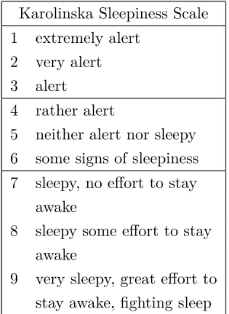
The Karolinska sleepiness scale is similar to the Stanford sleepiness scale, but divided into nine levels instead of seven [2]. The meanings of these levels are given in Table 2. In the original study, levels 2, 4, 6 and 8 had only ticks, but no labels. The answers given by the responents were validated against spectral analysis of EEG and visual analysis of electrooculogram in search of slow rolling eye movements.
Another interesting study searching for biomarkers of sleep is the one done by Seugnet, Boero, Gottschalk, Duntley and Shaw [64], where the amylase found in saliva was used to detect increasing levels of sleep debt. In the original study, the levels of amylase were studied on flies which were kept awake with caffeine and methamphetamine. After identifying amylase as a candidate for a biomarker indicating sleep debt, the research group measured the amylase levels of human subjects who were kept awake for twenty-eight hours during a two-weekend test period. Clearly this needs further studying. It is obvious, however, that there is a keen interest for finding a biomarker
that could indicate the level of drowsiness in people in a convincing manner.
2.3 Statistical Methods in Drowsiness Detection
Karolinska Sleepiness Scale 1 extremely alert
2 very alert 3 alert 4 rather alert
5 neither alert nor sleepy 6 some signs of sleepiness 7 sleepy, no effort to stay
awake
8 sleepy some effort to stay awake
9 very sleepy, great effort to stay awake, fighting sleep
Table 2: Karolinska Sleepiness Scale
In this chapter, I will show four different studies that apply statistical methods to measured EEG signals in order to detect signs of drowsiness. After these, I will focus in more depth on a study where a group is analysing speech using support vector machines, a machine learning tech-nique and finally a study where a balance board is used to measure the postural bal-ance and this data is then used to measure drowsiness.
Vuckovic, Radivojevic, Chen and Popovic [71] used an artificial neural net-work to recognise alert and and drowsy sequences. They used forty-two features from a cross-spectral density analysis to train an artificial neural network to de-tect drowsiness from an EEG signal. First
they used two neurologists to find sixty alert and sixty drowsy one-second epochs for each seventeen subjects. Only epochs that were selected by both neurologists were used as a sample. The subjects were allowed to proceed to stage one of sleep, but woken up before advancing to further stages.
Short periods of sleep were excluded from the material and only sam-ples without signs of sleep were used. The research group performed four experiments with sixty clear samples of alert and drowsy EEG, and finally a five-minute recording of raw EEG signal selected from the thirty-minute recording per each subject. In the first four experiments they used twenty of the selected sixty samples as a training set and forty alert and drowsy as validation set. In a final experiment the artificial neural network was measured against the two experienced neurologists.
Table 1 lists typical Alpha activity in alert subjects as activity in the range of 8-13 Hz. A cross-spectral density analysis [26] groups the activity of each spectrum and thus reveals if there is activity below or above the Alpha
range. The forty-two derived features were then fed into the neural network in order to produce a classifier that would identify if given a one-second epoch shows sign of drowsiness or not.
Three different neural networks were used. Linear network trained by Widrow-Hoff rule, feed-forward network trained with the Levenberg–Marquardt learning rule, and a learning vector quantisation rule were used. In these networks the data flows only to one direction and the difference is how the weights of the connections are updated.
The Widrow-Hoff rule [72] uses a least mean squares approach by starting with zero weights and updating them with the use of the mean square gradient. The Levenberg–Marquardt algorithm solves the problem of minimising a nonlinear function and this helps in finding the optimal nonlinear activation function for each neuron. Learning vector quantisation is a prototype-based supervised classification algorithm that was invented by Teuvo Kohonen [39]. First a self-organising map is used to find prototypes which are then learned by using the learning vector quantisation.
This method requires that the used epochs are selected in such a way that the groups of drowsy and alert are clearly separable. Mardi, Miri Ashtiani and Mikaili [50] has however developed a method that doesn’t have this limitation. The researchers calculated fractal dimension of the EEG signal using Higuchi’s algorithm [33] and the Petrosian’s algorithm [59]. A third feature used was the sum of squared logarithms of energy. These three features were used to train a feed-forward artificial neural network.
The research group recorded three or four forty-five-minute simulated driving sessions with ten drivers, who had been awake for at least twenty hours before the test. The drivers drove in a simulator, trying to avoid obstacles placed along their way. If the driver managed to pass the appearing barriers, they were considered to be in a state of alertness. If crashes happened, the driver was considered drowsy.
The four seconds leading up to a crash were always labelled ‘drowsy’ and the two following seconds as ‘alert’, since the simulator played a loud alarm for each crash, thus dispelling the driver’s drowsiness. Each crash event was reviewed, and if the subject said that they had been vigilant or if the video showed signs of drowsiness even though the person passed the barrier, then the event was not used as a ’drowsy’ example.
the EEG and extracted two-second epochs that were synchronised to show either a passing or a crash. Each drive was then split into two-second epochs. Finally, altogether 1686 observations were used. 80% of the data was used to train the classifier and the remaining 20% to test the performance of the classifier. This classifier was then used to achieve a two-class classification with an accuracy of 83.3%.
Independent component analysis [38] seems promising tool for finding a signal from a noisy source. The classical example used is the so-called cocktail party problem [17]: being in a noisy room with many people and wanting to hear the voice of the person you are talking with. Similarly, an EEG signal is recorded from many points of the scalp, and independent component analysis can be used to separate the different signals.
Everything shows up in EEG recordings: blinking, movements of the tongue, heartbeat. . . While driving can seem like a monotonous task, there are all kinds of things that happen inside a person who’s driving. This is where the independent component analysis brings out its best qualities. It helps to distinguish local fluctuations, caused by various sources, from the underlining base rhythm.
Lin, Wu, Liang, Chao, Chen and Jung developed an estimator for drowsi-ness using independent component analysis to filter out noise from measured EEG signals and by linking the brain activity to actual driving performance with the use of a power-spectrum analysis and a linear regression model [44]. They measured EEG from sixteen drivers driving a car for forty-five minutes. The measurements were made in the early afternoon hours, when the circadian rhythm has its second peak.
The researchers created their own metric for estimating driving perfor-mance. The driver was instructed to keep the vehicle as close to the centre line as possible, while the simulator was made to cause seemingly random events of sudden changes in steering wheel angle in order to simulate driving on a bad road. These deviations were used to measure the corrective actions that the driver undertook in order to keep the vehicle on course. Five of the sixteen drivers were selected for further study because of the microsleep intrusions detected in their first driving session.
The research group found that drowsiness fluctuates with cycle lengths of more than four minutes and used a moving average filter advancing two seconds at a time to eliminate variance at shorter cycle lengths. After
filtering out the EEG artefacts using independent component analysis the power-spectrum of the EEG was analysed. From the data thus produced, a correlation coefficient was computed using the Pearson product-moment correlation coefficient. The group found out that the log power spectra of two components in the range of 9–25 Hz had a strongly positive correlation with the performance of the driver.
Overall, the group had a success rate of 86.2% for the training session and of 88.2% for the test session when two dominant independent component analysis components were used as input features to a linear regression model for the selected five subjects. The researchers noted that the relationship between the brain activity shown in the EEG data and actual driving performance remained stable from session to session for each driver, but varied somewhat between different drivers.
The biggest obstacle for using EEG for drowsiness detection is the dif-ficulty in getting a signal from the driver. EEG requires twenty-four to thirty-two electrodes and it’s not feasible to do a large scale study with the current equipment. All kinds of devices have been proposed, and currently there are more than ten projects on the crowdfunding website Kickstarter seeking funding for an EEG recording device.
Another possible use for EEG signals is the brain-computer interface. Lin, Chang, Lin, Hung, Chao and Wang have proposed a lightweight headband [43] that uses EEG signals to detect drowsiness. The aim of the group was to develop a brain-computer interface that would have the same benefits as devices that focus on the physiological signs of drowsiness, such as eye cameras and grip strength. The main benefit of these is that they don’t require contact and are thus easier to accept.
The group also wanted to obtain the qualities of another group of devices that measure the physiological signs of drowsiness, like the electric potential of skin and EEG activities. These devices are less dependent on things such as lighting conditions, vehicle type or driving conditions.
A signal reading module consists of the following components: three EEG electrodes that read brain waves in the occipital midline, a signal amplifier, a band-pass filter, an analogue-to-digital converter and finally, a bluetooth module that sends the processed data to a microprocessor that can then alert the driver in real-time if dangerous drowsiness is detected.
Batliner and Golz studied how speech changes when a person gets more tired and applied machine learning to detect these signs of drowsiness [41]. The group used a support vector machine that was trained to classify speech into alert and drowsy with good accuracy.
The researchers hypothesised a number of changes that they thought would be caused by drowsiness. Their first assumption was that cognitive speech planning would become impaired as a person grows tired, thus affecting the speed of speech as well as slurring the articulation and increasing errors. A second assumption was that the decreased muscle tension that causes flat and slow respiration would cause observable changes in phonation and articulation. Thirdly, the relaxed open mouth display caused by drowsiness would have an effect in the first and second formant position.
Krajewski, Batliner and Golz recorded twelve student volunteers, who participated in an all-night study with an hourly routine consisting of forty minutes of driving, fifteen minutes of vigilance tests, responding to the Karolinska sleepiness scale questionnaire, two minutes of recording speech and a break. For each student, seven sessions in total were conducted between one a.m. to eight a.m. The voice recordings made during the night were split into alert and drowsy samples by combining them with the information provided by the Karolinska sleepiness scale questionnaire, with a threshold of 7.5. This threshold was validated by the presence of microsleeps, which did not occur during alert phases.
Speech data has usually a high number of features because often data is split into ten millisecond frames and smoothed. Data was then analysed frame by frame using signal processing, speaker-recognition and speech-recognition-based acoustic features. The final dataset had over forty-five-thousand dimensions, which were reduced to two-hundred-and-thirty features by using a simple correlation-filter-based feature subset selection.
Finally, the group compared thirteen different classifiers, and the support vector machine managed to correctly classify 86.1% of the samples into alert or drowsy. Class-wise, the average classification performance was 82.8%. Logistic regression [48] was a close second, while the two nearest neighbours classifier [18] and the random forest classifier [13] had the worst performance with overall performance of 62.8% and 68.1% and class-wise averaged performance of 69.5% and 62.9%, respectively. These results required the speaker to be known.
Another promising idea for detecting drowsiness is to use the Nintendo® Wii Fit balance board to measure a person’s postural steadiness [68]. This has been tried out in one study, where the balance board was used to measure the postural steadiness of fifteen test subjects every hour during a twenty-four-hour test period. The tested subjects were offered a snack or a light meal every two hours.
The score derived from measuring the subjects’ postural steadiness was tested against a ‘drowsiness baseline’ that the group created by using the Stan-ford sleepiness scale and an estimation of alertness based on a three-process model that combines homeostatic, circadian and sleep inertia components. The three-process model predicts that alertness peaks seven-and-a-half hours after waking up and at half-past-three in the afternoon, and that drowsiness peaks after staying awake for twenty-two-and-a-half hours and at half-past-six in the evening [1].
The group used multiscale fuzzy sample entropy [76] to extract features from the signal originating from the balance board. The result was a complexity index, which measures the predictability of the signal. Each test consisted of four thirty-second tries during which the person stood on the board and tried to maintain their balance.
For the times considered as alertness peaks by the three-process model, the complexity index group average was 8.9±1.3. For the drowsiness peaks, it was 7.9±1.4. The values given by the Stanford sleepiness scale were 2.0±0.7 (from one to three) for the alert peaks, and 4.8±1.1 (three to six) for the drowsy peaks. Overall, the correlation between the complexity index and predicted alertness wasp= 0.94.
The most promising thing about using the balance scale for measuring drowsiness is that it is very practical in field use, similarly to the breathalyser used for measuring drunkenness. Law enforcement personnel could carry the board with them, and driving sleepy could become as easily penalised as driving drunk.
Next I will show how the results and methods presented here are used as a baseline in order to study drowsiness in drivers. Many studies take place in a laboratory settings where quick drowsiness detection methods like psychomotor vigilance task and questionnaires precede and succeed periods of driving. EEG and self-reported drowsiness can be recorded when studying real driving.
3
Evaluating the Driving Performance of the Driver
Here I will show how metrics for driving performance have been developed using biomarkers from previous chapter as a baseline. I will first take a look at how drowsiness affects driving performance. I will then describe ways how drowsiness can be detected with measurements made in the car that is being driven. Finally, I will take a look at current research and modern solutions for detecting drivers’ drowsiness.3.1 Psychological Issues Related to Driving Performance Driving is a complex task that requires situational awareness [25]. A car moving 100.8 km/h travels 28 metres per second. Drowsiness in such speeds can pose a real danger. A project led by the European Commission identified a number of psychological symptoms related to fatigue [63]. They listed such symptoms as decrease in vigilance, slower reaction time, poor memory, worse psychomotor coordination, slower information processing, and poor decision making.
Studies have shown that driving in a monotonous environment causes large steering wheel movements to become more frequent [67]. This is consistent with what the SafetyNet project has also reported. Drivers tend to notice when they get tired and try to compensate this in two ways: either by driving faster to increase the demandingness of the task, or by slowing down and keeping a bigger distance to other vehicles in order to compensate for longer reaction times [63].
The circadian rhythm also affects the driver [42]. Due to this evolution-based rhythm, a human’s desire to sleep is strongest from 2 a.m. to 4 a.m. and again between 2 p.m. and 3 p.m. Alertness is highest at 10 a.m., eye-hand coordination at its best at 2:30 p.m. and reaction times shortest at 3:30. These aspects are further discussed below.
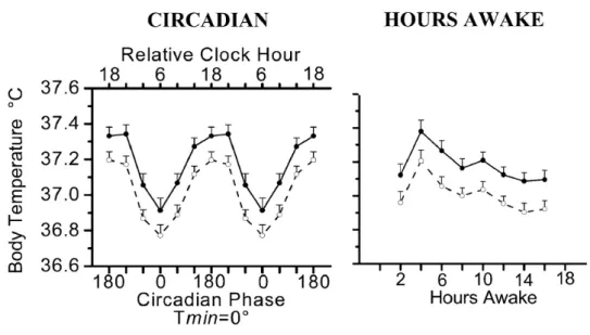
Wright, Hull and Czeisler studied the relationship between alertness, performance, and body temperature [75]. In their study, the testees’ day was stretched to a twenty-eight-hour cycle consisting of eighteen hours and forty minutes of scheduled wakefulness and nine hours and twenty minutes of scheduled sleep. The fourteen participants were made to live by this rhythm for twelve cycles in total, corresponding to fourteen normal days. The subjects were asked to do a thirty-minute battery of tests every two
Figure 4: Average high and low body temperature of 14 subjects across 24 h circadian phase (left) and hours awake (right). Solid line for High and double dotted for low. Error bars represent ± standard error. Copyright © 2002 the American Physiological Society
hours, starting two hours after the beginning of the scheduled wakefulness. The researchers knew that the human body cannot maintain a eight-hour day under selected conditions, and that it will continue its twenty-four-hour cycle thus enabling the researchers to study the circadian rhythm with different waking times. The participants body temperature, which was measured once a minute, varied roughly by one degree celcius, while the temperature and lighting conditions of their surroundings were kept unchanged. Sixty degrees is four hours in this twenty-four-hour clock face.
Dijk, Duffy and Czeisler studied alertness with two groups of participants. One group was kept awake by a constant routine for a total of thirty-six to sixty hours after an initial synchronisation phase. This group showed fairly consistent mental performance for the first sixteen hours. After that, their mental performance correlated with the circadian rhythm and with the low point of the temperature cycle [21].
The other group had a twenty-eight-hour routine similar to the one described above. The self-reported minimum level of alertness for this group coincided with the body temperature minimum, and mental performance minimum followed shortly after. The testees’ did not show the expected
Figure 5: Circadian phase-dependent (left; data double plotted) and hours awake-dependent variation (right) of addition performance. Neurobehavioral data are expressed in deviation from individual subject’s mean. Scores in the upward direction represent better performance. The group mean (n = 14) is added to the high-low deviation scores to indicate the amount of change in performance. Error bars represent ±standard error. Dotted line represents the group mean. Copyright © 2002 the American Physiological Society
mid-afternoon drop in either alertness or mental performance. The testees’ mental performance was assessed by having them perform an hourly test that consisted of adding pairs of two-digit numbers.
Wright, Hull and Czeisler had their participants do this same task as well, and Fig. 5 shows how the performance of their testees varied according to different phases of the circadian cycle and to hours of staying awake [75].
Being able to react fast in surprising situations is vital for drivers. The fact that reaction times vary according to the time of the day is also essential to keep in mind while searching for ways to improve driving safety. Reinberg, Bicakova-Rocher, Nouguier, Gorceix, Mechkouri, Touitou and Ashkenazi [62] studied the daily variation of reaction times by comparing those of the driver’s dominant and non-dominant hand. Their hypothesis was that there is a difference in the rhythm of the daily variation of reaction times between these two hands, and their research showed that this is indeed the case.
The group tested eleven testees with a simple reaction test: a yellow light was shown to the testee, and the time it took for the testee to press a button after seeing the light was measured. A three-colour setup was also used, where the subject was required to press the button with their left hand at the appearance of one colour, to press it with their right hand at the
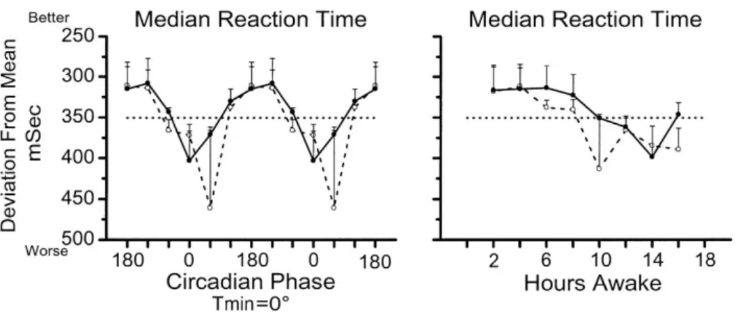
Figure 6: Circadian phase-dependent (left; data double plotted) and hours awake-dependent variation (right) of median reaction time in Psychomotor Vigilance Task performance associated with high vs. low body temperature. Copyright © 2002 the American Physiological Society
appearance of a second colour, and to ignore the third colour. The test, in which ninety-six signals altogether were given, was done from four to eleven times a day for each testee, during twelve to fifteen days. The testees’ reaction times were noted to vary by around 20% depending on the phase of their circadian rhythm.
Wright, Hull and Czeisler et al. used the psychomotor vigilance task as a part of their assessment for drowsiness and for the effects of the circadian rhythm [75]. Figure 6 shows how the median reaction time was noted to vary across the circadian phase and how this was further influenced by how long the testee had been staying awake. The median reaction time varies from 300 to 400 milliseconds. During this difference of 100 milliseconds, a car driving a hundred kilometres per hour advances three metres.
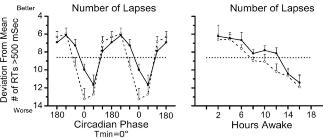
Figure 7 shows how the number of lapses, or responses that took more than 500 milliseconds to react to a stimulus, increases first, dips during the afternoon hours, then rises again and finally decreases quite rapidly after having been awake for twelve hours.
Edwards, Waterhouse and Reilly studied the effects of the circadian rhythm on alertness with a game of eye-hand coordination. In the game that they devised, a small disc is flicked in order to hit a target at the distance of thirty or fifty centimetres [23].
Figure 7: Circadian phase-dependent (left; data double plotted) and hours awake-dependent variation (right) of number of lapses in Psychomotor Vig-ilance Task performance associated with high vs. low body temperature. Copyright © 2002 the American Physiological Society
attempts at the shorter distance target first, and then another round of twenty tries at the longer distance target. In total, the test took less than ten minutes to complete, and it was performed six times with each student, with 28-hour intervals. Each throw was scored on a scale of zero to six, and the first three and final three throws were excluded to eliminate the effects of a possible anxiety related to starting and finishing the task.
The accuracy of performance for both the short- and the long-distance shot motor task showed a correspondence between the circadian rhythm and the subjects’ measured core temperature and self-reported alertness and fatigue scores, which were measured using a visual analogue scale. Performance was at its best at 4:00 p.m., when the range of mean scores reached from seventeen to twenty-four in the short-distance task and from fourteen to twenty in the long-distance task.
The study was repeated to see if there was a difference between the dominant and non-dominant hand in the effect of the circadian rhythm, as suggested by Reinberg et al. A similar pattern was found in this second study, where seventy-eight students were made to perform the same task as described above [24].
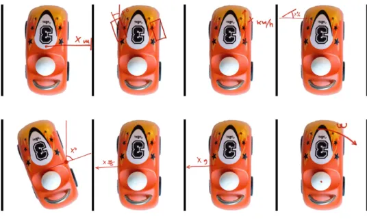
Figure 8: Eight sources of data: (from top left) lateral lane position, steering wheel angle, speed, accelerator pedal position, yaw angle, lateral velocity, lateral acceleration, and angular velocity.
3.2 Biomarkers for Driver Drowsiness
Forsman, Vila, Short, Mott and Van Dongen evaluated eighty-seven different metrics for detecting a driver’s drowsiness on the basis of data provided by measurements done on the car that is being driven. The group identified eight different sources for such data [28]: the car’s (1) lateral lane position, (2) lateral velocity, (3) lateral acceleration and (4) angular velocity, the car’s (5) speed and (6) yaw angle, (7) the position of the accelerator pedal and (8)
the angle of the steering wheel.
The lateral lane position is typically measured with a camera that records a view of the road on video. The distance of the car to the lane markings is calculated from this video. The study group listed twelve variables for using lateral lane position to detect drowsiness. The (1) mean value can reveal if the driver starts to compensate for drowsiness by driving closer to the centre line or nearer to the other side. Standard deviation (2) and (3) variance will show how the values are spread around the mean value.
Root-mean-square (4) of the lateral lane position can also be used, as well as the (5) signal-to-noise ratio, which here is the reciprocal coefficient of
variation of signal variability. These five variables are calculated from all sources of data, with the exception of the yaw angle.
The rest of the variables that can be calculated from the lateral lane position include the three variables that are used to measure signal deviations: (6) the total signal deviation from windowed signal average, (7) the average signal deviation from windowed signal average and (8) the variance of signal deviations from windowed signal average. These three use a twenty second window to detect anomalies in the signal.
Signs of drowsiness can also be observed from (9) the most common signal frequency, as well as from (10) the energy or power of the signal. Finally, there are two variables that estimate how long it would take for the car to cross the lane boundary if no steering corrections are made. These are (11) time to lane crossing within six seconds and (12) time to lane crossing within sixty seconds. The standard deviation of the lane position was stated by the group as the most important indicator for a driver’s drowsiness measured from the vehicle, along with steering wheel movements [45].
Among the eight sources of data identified by Forsman et al., the steering wheel angle is the one with the greatest number of variables. All the variables that have been used to detect drowsiness by measuring the lateral lane position have also been used in relation to the steering wheel angle. In addition to these, there are twenty-six variables more that Forsman et al. identified in their review.
Fifteen of these twenty-six variables are related to signal amplitude. Five of these fifteen calculate a percentage of samples with signal amplitude exceeding levels of 0.3, 3, and 30 degrees and 1, and 2 standard deviations. There are variables for maximum signal amplitude to the right and left, cumulative signal amplitudes to right and left, and percentages for samples with signal amplitude to right/left.
Finally there are variables with most common signal amplitude to right and to left and corresponding variables for percentage of samples with those amplitudes. Eleven remaining variables for steering wheel angle are: degree of interaction between steering wheel angle and yaw/lateral acceleration, number of steering wheel direction reversals, average radius in phase-plot, arc length of phase-plot, area of phase-plot, entropy of central/right/left steering movements, fractal dimension of signal, and reaction time from signal auto-/cross-correlation with yaw of the car.
Vehicle speed can also reveal drowsiness. The SafetyNet project discovered that drivers tend to compensate their tiredness by either driving faster to increase the demandingness of the task or by slowing down and keeping a bigger distance to other vehicles in order to compensate for longer reaction times [63]. Mean value, variance and standard deviation have been used to study drowsiness on the basis of vehicle speed, as well as root-mean-square and signal-to-noise ratio.
The time to lane crossing is calculated from vehicle speed for both six and sixty seconds. Fractal dimension shows the complexity of the curve drawn from the values. Basically, this shows if the driver suddenly changes from making many small corrections to making fewer but larger corrections. The hypothesis is that this tends to happen when the driver starts to lose their focus and coordination.
The variables unique to this biomarker are the three measures of devia-tions from 55 mph. These are (1) an average of signal deviadevia-tions, (2) standard deviation of signal deviations, and (3) reciprocal coefficient of variation, or signal-to-noise ratio of signal deviations from 55 mph.
The accelerator pedal position is closely related to the speed of the vehicle, but it can show the effects of growing tiredness faster. Mean value, variance and standard deviation have been used to detect drowsiness on the basis of accelerator pedal position, as well as the root-mean-square and signal-to-noise ratio. These five variables have also been used with lateral velocity and lateral acceleration. The latter of these has also been used in connection with the steering wheel angle to calculate the degree of interaction between different types of signals. This degree of interaction is the distance of normalised variables, and it measures how well the driver and the car interact [47].
Angular velocity is a measurement for how fast the car is changing its direction. In addition to mean value, variance, standard deviation, root-mean-square and signal-to-noise ratio, maximum amplitude to right and to left have been used as a possible biomarker for drowsiness. The most common amplitude to both directions, as well as the percentage of values matching that value, have been used in research as indicators for drowsiness.
The phase-plot or phase portrait of the angular velocity values is a source of data used in relation with the remaining three variables identified by Forsman et al. Average radius, arc length and area of the plot can provide
insight and reveal, for example, how steady the velocity of the vehicle is. If the arc length grows, but the mean stays the same, this indicates that there are a lot of changes in the signal value.
The yaw angle, or the direction where the car is heading, measures the orientation of the car in relation to the road. Six variables have been used in previous research to detect drowsy driving on the basis of the yaw angle. The most common signal frequency of the yaw angle can offer better sensitivity compared to the lateral lane position by telling which way the car is headed. The energy of the signal is the root-mean-square to the second power. Much like with variance and standard deviation, the reason for using a multitude of variables has to do with the scale of the values.
The time to lane crossing can be calculated from the yaw angle and vehicle speed as well. This measurement has been used with values of six and sixty seconds. Reaction time can be estimated by cross-correlating it with the steering wheel angle. Finally, the degree of interaction with the steering wheel angle tells how well the driver and the car are in sync. Large corrections that result in lots of smaller corrections for the initial correction can reveal drowsiness.
The aim of the research done by Forsman et al. was to compare different proposed metrics for detecting a driver’s drowsiness on the basis of data provided by measurements made on the car, and to develop a method for detecting moderate levels of drowsiness instead of a grave and imminent problem like having fallen asleep at the wheel. In Forsman’s study, forty-one tested participants lived inside the laboratory for fourteen days with either a night-shift or a day-shift work.
Participants were tested four times each day. During each testing period, they were first tested with a ten-minute psychomotor vigilance test, were then made to drive for thirty minutes, and another psychomotor vigilance test after the drive. The test was completed by a short neurobehavioral test battery that included a self-reported drowsiness score and a visual analogue scale for the mood along with many different tests that measure for instance reaction times and the ability to substitute digits with symbols in order to detect their fatigue.
Principal component analysis was used to reduce the dimensionality of the data across all participants to include only measures concerning steering wheel variability and lateral lane position. Lateral lane position also correlated the
most with the participants’ performance in the psychomotor vigilance test which is an oft-used method for measuring drowsiness. Eight curved road segments were used to validate these findings in each driving session.
They also showed that the lateral lane position could be derived from steering wheel angle measurements using transfer functions. This was an important step because the lateral lane position requires the lane markings to be visible to the camera. The visibility of the markings could become a problem for example on roads covered with snow. Forsman’s research suggests that the steering wheel could be used alone to develop a biomarker for driver drowsiness.
3.3 Existing Solutions for Detecting Drowsiness in Drivers Morris, Pilcher and Switzer proposed a model for detecting drowsy driving with the use of retrospective analysis around curves [55]. According to their research, the yaw angle (vehicle heading difference) performed best in detecting drowsiness that was measured using psychomotor vigilance test and fitness impairment tester. Fitness impairment test measures the eye saccade velocity in a thirty second test. Researchers were able to detect significant differences in driving performance in eight of the ten test sessions.
In Morris’ group’s study, twenty college students were kept awake for twenty-six hours and made to drive five twenty-minute test sessions in a simulator during one day, starting at eight p.m. and finishing at ten a.m. The testees were woken up at a pre-determined time between eight a.m. and ten a.m., and waking up was confirmed with a phone call. A total of thirty-seven different variables were recorded from the car during the test sessions at a rate of one Hz.
A psychomotor vigilance test was administered on the testees once during each test session, and a fitness impairment test was completed twice before and twice after each session, with a five-minute break in between. Measured reaction times and numbers of lapses were noted to increase in each mea-surement, as was to be expected on the basis of current understanding on how staying awake affects humans. Saccadic movement of the eye is normal, jerky, motion of the eyes. The speed of the movement slows down as the person gets more tired. The speed of this movement decreased in the testees, as was expected.
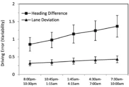
Figure 9: Driving variability over the night for lane deviation and heading difference (mean ± stan-dard error). (Image from Morris, Pilcher, and Switzer [55] © 2015 Elsevier Ltd.)
Figure 10: Number of lapses (re-sponse time >500 ms) from psy-chomotor vigilance task (mean± standard error). (Image from Morris, Pilcher, and Switzer [55] © 2015 Elsevier Ltd.)
difference was noted to be a better indicator than lane deviation (see Fig. 9 above). The research indicated that once people grow more tired they start to make fever but bigger corrections as they drive through turns. The method that was noted to be most reliable was able to detect a significant difference in the means of eight of the ten compared test sessions.
The research group tried both root-mean-square error from the absolute difference and the standard deviation formula for both measurements and the results varied from six of ten with root-mean-square and lane position to the eight of ten with root-mean-square of heading difference. Both got seven of ten with standard deviation formula.
The mean of heading difference seems to grow, but the error is pretty high compared to lane deviation. Figure 10 shows how the number of lapses in a ten-minute test grows from roughly two to more than seventeen on average. Heading difference, measured in degrees, shows the relation of the yaw of the car and the tangential direction of the lane.
In another study, lane departures in a simulator were used as biomarkers and McDonald, Lee, Schwarz, and Brown [53] wanted to learn to classify the last sixty seconds of driving before the event and a matched sample of alert driving on the same road segment. Researchers used supervised machine learning and trained the classifier with carefully chosen samples of driving. Their goal was to develop a method to alert the driver before a lane departure.
Seventy-two participants took part in the study. They drove three thirty-minute rides in a simulator. The faces of the testees were filmed as they were driving, and each lane departure was manually scored by using an observer rating of drowsiness [73]. The threshold for a departure to be considered drowsy was thirty-seven, corresponding to ‘at least a moderate level of drowsiness’. Each drowsy departure was matched with data from the same road segment, and if possible, from the same driver. The final six seconds leading up to the lane departure were removed because the researchers’ aim was to create a system that could alert the driver beforehand.
The drivers’ level of alertness was confirmed using a modified psychomotor vigilance task, the Stanford sleepiness scale and a retrospective sleepiness scale. Only drivers who passed as alert in all three measures were qualified as alert samples. The final evaluation data set included eighty alert samples of a same driver and another 336 samples of other drivers on a same road segment as the 162 drowsy sample.
The study group used seven different classifiers and measured the success of each classifier using a receiver operating characteristic, which is a curve of true positive rate in the y-axis against the false positive rate in the x-axis. Two such plots were compared by calculating the area under the curve. Figure 11 shows the random Forest classifier compared against other six classifiers.
Decision tree [35] is used to classify new unseen data based on training data set that is labeled. From the training set a binary tree is constructed by creating splits like ’steering wheel angle is greater than five degrees’ or ’distance from the centre point is greater than one metre’. Each split-line is a binary choice and each new data point is then taken to the right leaf where a majority vote decides the label for this data. In this study the depth of the tree was limited to six.
Random forest [13] is a collection of decision trees that have been trained on a different parts of the training set in order to reduce variance. Bootstrap aggregating, or bagging [11], generates new training sets by sampling from the original training set uniformly with replacement. This is called bootstrapping and it’s a useful way to estimate the accuracy of an estimator. Here McDonald, Lee, Schwarz, and Brown used five-hundred trees with forty-one features for each iteration.
Figure 11: Receiver operating characteristic comparison plots for the random forest (RF) model and the six other models. From left to right, top to bottom, the figure shows the following models: decision tree (DT), neural network (NN), support vector machine (SVM), naive Bayesian (BN), k-nearest neighbour (kNN), and boosted tree (BT). Copyright © 2013, Human Factors and Ergonomics Society
decision tree is trained with training data, but all of the misclassified data is taken away and used to train another tree. This is repeated until all of the training data has a tree that classifies it. For classification, a weighted vote is used to give the new data point a label. Earlier trees are given larger weights, and each subsequent tree gets a lower share of the vote. In this study, the researchers used 0.1 as the decay value.
A fourth classifier tested was a neural network [52]. It is made of interconnected layers of nodes, and each connection has a weight. A node can be thought as a representation of a sigmoid function to the sum of the output of previous nodes. Weights are updated in a process called backward propagation of errors, or backpropagation. McDonald, Lee, Schwarz and Brown used two hidden layers and 0.1 as the training weight decay.
The k-nearest neighbours classifier [18] memorises the training data. For new data, it just takes k closest matches and assigns the label for the data by taking a majority vote on those matches. The search group used nine as the value of neighbours to classify unseen data into alert and drowsy drives.
Naive Bayes’ classifier builds upon Bayes’ theorem [8] for events A and B. If we detect B and want to know what the probability for A given B is then we can use the Bayes’ theorem:
P(A|B) = P(B|A)P(A)
P(B)
to come up with conditional probabilities. The classifier gives the label from the event associated with the highest conditional probability as its answer. Finally, a support vector machine [69] was used to try and fit a hyperplane between the alert and drowsy samples. This was done in order to produce a classifier that could be used to predict new data by looking at its features. Original data is often not separable, but it can be made separable by adding dimensions which help to classify the data.
In the end, the random forest performed best with an area under curve of 0.7. The other classifiers were in the range of 0.63 to 0.66 with the exception of Naive Bayes’, which performed worst. The Naive Bayes’ classifier was the only one that was beaten by the random forest with statistical significance. The random forest classifier was then compared to an algorithm that measured when the eyes of the driver were closed. It had a three-minute window and a threshold of seventy percent for eye closure. It calculated how
much of the three-minutes the eyelids covered more than seventy percent of the eyes. This setup gave the best area under curve of 0.63. Mean accuracy was 0.55 and 0.79 for the eye closure algorithm and random forest classifier, respectively.
A lot of research has focused on detecting drowsiness from EEG data. Yeo. Li, Shen and Wilder-Smith presented an EEG-based drowsiness detector [77] that reached 99.3% classification accuracy for unseen data, with human scored drowsiness used as a benchmark. In Yeo’s study, twenty students from the National University of Singapore drove in a simulator and had their EEG recorded with the use of a thirty-two-channel system with 256 Hz sampling frequency. The one-hour drive was done during the afternoon sleepiness peak at three p.m.
The research group used support vector machines to learn how to detect drowsiness from EEG data after carefully selecting the training data by looking at eye blinks and EEG frequency. They then extracted four variables: dominant frequency, average power of dominant peak, centre of gravity frequency, and variability. Finally, they used two different raters and only included epochs where both of these agreed on the alertness or drowsiness of the epochs.
4
Learning to Predict Sleepiness on the Basis of
Car Data
In 2013, there were 197 motor vehicle accidents in Finland that resulted in loss of life. Thirty-nine passengers and 173 drivers were killed in these accidents [40]. The Finnish Motor Insurers’ Centre publishes statistics on the causes of motor vehicle accidents, and according to them, seventeen of the accidents that happened in 2013 were caused by loss of alertness or because the driver had fallen asleep [40]. According to the estimates of the World Health Organization, there are 1.25 million deaths worldwide each year that are caused by traffic accidents [74].
In Finland, it is illegal to drive if you are too tired. However 92.5% of the drivers punished under Article 63 of the Road traffic act in 2004 and 2005 were involved in an accident [60]. Radun, Radun and Ohisalo found no cases where the driver would have received a penalty in a random stop. There appears to be no way to detect dangerous drowsiness before the driver
actually falls asleep.
Professional drivers transporting commercial goods or passengers use tachographs to record their driving hours, which are limited by European Union regulation. This is currently the best available tool to prevent drowsy driving. People continue driving even when they know they are too tired to drive. In a 1520-person study, conducted by TNS Gallup in the spring of 2013 for the Finnish Road Safety Council Liikenneturva, 26% of the drivers reported having fallen asleep at least once and 95% having driven even when they knew they were tired [49].
Earlier on in this work, I described the research led by Pia Forsman [28] in which eighty-seven sleepiness indicators were identified that had already been observed in various studies over the years. I will now show how supervised machine learning can help in detecting drivers’ drowsiness.
Previous research has mainly focused on detecting dangerous drowsiness just before an accident. As seen in previous chapters, all kinds of data has been used for this purpose, produced by measurements performed both on the driver as well as on the car. Here my aim is to use data recorded on a daytime drive to predict which drivers will fail to continue their driving because of dangerous drowsiness. Data about the driver will only be used to train the classifier, while for the actual prediction, the classifier will be shown data concerning the car, or more specifically, the car’s steering wheel, speedometer and accelerator pedal.
4.1 Data Source and Measurements
The data used in this study is from a study done by Torbjörn Åkerstedt, David Hallvig, Anna Anund, Carina Fors, Johanna Schwarz and Göran Kecklund, who used the same data in their study on driving at night and dangerous sleepiness [3]. They studied the development of indicators for dangerous drowsiness that led to the termination of a night-time drive by either the drivers themselves or by the accompanying test leader .
The group did their study with eighteen individuals who were randomly chosen among the vehicle owners registered in Sweden and living in the region of Linköping. These testees were first made to drive during the afternoon for roughly eighty kilometres towards Nyköping, and then back along the E4 motorway. After seven hours of resting in a controlled environment, they were made to drive the same route again. In the original study, EEG and
electrooculogram were identified as the best sources of information about drowsiness.
Each driver had a test leader alongside them when they drove. The setting was fairly strict: any request for a break resulted in the termination of the drive, and the driver was instructed not to speak to the test leader. The only moment when the driver was allowed to talk was when the test leader asked them to evaluate their feelings of drowsiness with a number from one to nine, which was done every five minutes.
Eight of the eighteen night-time drives were terminated prematurely – two by drivers themselves and six by the test leader. Three of these eight reported having fallen asleep and, alarmingly, one of the ten drivers who finished the drive also reported as having fallen asleep during the drive even though the test leader had had a view of the driver’s face. There was no sudden increase in any of the indicators immediately before the critical event, but rather a steady increase in several indicators.
The daytime drive was done between 15:30 and 19:15 and the night-time drive on the following night, between 00:15 and 04:15. The wide window for the sessions to take place was caused by the fact that two drivers were tested each day. All of the drivers were also asked to keep a sleep diary during the three days preceding the day of the driving sessions.
Figure 12: Experiment set up showing eighteen drivers driving for ninety minutes at a time first during the day and then during the following night.
The aim of the study was to detect moderate levels of drowsiness instead of the extreme dangerous ones. The drivers were not allowed to drink caffeine or to listen to the radio, and if they wanted to take a break, the drive was terminated. The test leader travelled along during all of the rides, and the car was equipped with two sets of controls in order to allow the test leader to take over should the driver fall asleep. After the first drive, the testees were served dinner and then taken to a controlled environment where they could watch the television, read and interact socially with the research group.
Two sets of measurements were made during the drives. First, a number of measurements were made directly on the driver. These included EEG, electrooculography, electromyography and electrocardiography. The sampling frequency was 512 Hz for EOG and 256 Hz for others. Another set of measurements were made on the car that was being driven. Ten variables were produced by recording data from the GPS signal, while twenty other measurements related to the direction of the car and its position on the road, such as the distance travelled or the direction of the yaw of the car. The sampling frequency for measurements done on the car was 10 Hz. Table 3 lists all the variables produced with these measurements.
The researchers derived two additional variables from the measurements made on the driver. They calculated the Karolinska Drowsiness Score (KDS) [30] and used an algorithm developed by Jammes, Sharabty and Esteve [36] to calculate blink durations. Each twenty second epoch of driving was manually scored for signs of drowsiness in either the driver’s brainwaves or in the electrooculogram. Slow, rolling eye movements of at least 100µV and lasting for more than one second were marked as signs of drowsiness in the electrooculogram.
Each epoch was split into ten units of two seconds, after which the scorer searched each two-second segment for signs of drowsiness. The KDS for the whole twenty-second epoch is the number of these smaller segments that show physical signs of drowsiness so that an epoch with two segments containing drowsiness events gets a KDS of 20%.
Figure 13: Each twenty seconds is labelled with how much sleepiness the EEG and the electrooculogram show.
Table 3: Controller area network variables based on measure-ments made on the Car
variable name description precision
mAccelPedalPos How much the accelerator is pressed 0.1%
mAmbientLightCond ambient light on boolean
mAmbientTemp ambient temperature 0.01◦C
mDirInd direction indication
with oscillations removed {0,1,2}
mDistanceTraveled distance traveled 1m
mEngineSpeed engine speed 0.0001rpm
mGearSelected selected gear {0,1,2,3}
mInCarTemp in-car temperature 0.1◦C
mLateralAcc values from (-3.324 to 3.551) 0.0001m/s2
mLateralJerk lateral jerk 0.01 m/s3
mLeftLaneOffset left lane offset 0.01m
mLeftLaneQuality left lane quality boolean
mLongAccBackUp longitudinal acceleration 0.001m/s2 mLongAccSensor longitudinal acceleration sensor value 0.0001m/s2 mNumFixSatellites_GPS number of GPS satellite connections count
Table 3 – continued from previous page
variable name description precision
mOdometer odometer of the car 1km
mRightLaneOffset right lane offset 0.01m
mRightLaneQuality right lane quality boolean mSteeringAngle steering wheel angle 0.01◦
mVehicleSpeed vehicle speed 0.01km/h
mVideo0Indices frame index of video 0 count mVideo1Indices frame index of video 1 count mVideo2Indices frame index of video 2 count mVideo3Indices frame index of video 3 count mWiperFront front windshield wiper in use boolean
mYawRate yaw rate ◦/s
timeindex time index with a step of 100 0.001s timeSync time synchronisation index with a step of 100 0.001s timeNTP network time protocol time 0.00001s sleepinessExperiment marker to when the experiment is on boolean speedLimit90 speed limit is 90 km/h boolean dmLeftLineCrossings left line is crossed boolean dmRightLineCrossings right lane is crossed boolean dmLane 1 = right lane, 2 = left lane, {1,2,12,21}
12 = switching from left to right, 21 = switching from right to left
Table 3: Controller area network variables based on measure-ments made on the Car
4.2 Summary Statistics Used to Train a Classifier
Measured data is split into twenty second epochs and thirteen summary statistics is calculated from these epochs. From the fifty-two available measurements, I chose three as a basis for creating summary statistics. The selected measurements were the angle of the steering wheel, the position of the accelerator pedal and the speed of the vehicle. These were all measured at a frequency of ten Hz, so each twenty second epoch contains 200 values
![Figure 3: EMG recording of a rodent from Scholarpedia. Copyright © Christo- Christo-pher M Sinton [51]](https://thumb-us.123doks.com/thumbv2/123dok_us/1308314.2675044/9.892.176.713.161.498/figure-recording-rodent-scholarpedia-copyright-christo-christo-sinton.webp)