Czech Technical University in Prague
Faculty of Electrical Engineering
Department of Cybernetics
DIPLOMA THESIS
Visual Path Detection for Mobile Robot
Navigation
Author: Bc. Dina Sushkova
Advisor: Ing. Karel Košnar, Ph.D.
Czech Technical University in Prague Faculty of Electrical Engineering
Department of Cybernetics
DIPLOMA THESIS ASSIGNMENT
Student: Bc. Dina S u s h k o v a Study programme: Cybernetics and Robotics Specialisation: Robotics
Title of Diploma Thesis: Visual Path Detection for Mobile Robot Navigation
Guidelines: 1. Study methods for shadow removal from image. 2. Study methods for visual path detection.
3. Design algoritms for real-time path detection and robot control for path following. 4. Verify methods on public datasets.
5. Perform experiments with real robot.
6. Evaluate preformance of designed algorithms. Bibliography/Sources:
[1] Tomáš Krajník, Jan Blažíček, Joao M. Santos, "Visual Road Following Using Intrinsic Images", Mobile Robots (ECMR), 2015 European Conference on, vol., no., pp. 1-6, 2-4 Sept. 2015
[2] José M. Álvarez and Antonio M. López, "Road Detection Based on Illuminant Invariance", IEEE Transactions on Intelligent Transportation Systems, Vol. 2, No.1, March 2011
[3] G. Finlayson, M. Drew, and C. Lu, "Entropy minimization for shadow removal", International Journal of Computer Vision, 2009
[4] Hailing Zhou, Hui Kong, Lei Wei, Douglas Creighton, Saeid Nahavandi, "Efficient Road Detection and Tracking for Unmanned Aerial Vehicle", IEEE Transactions on Intelligent Transportation Systems, Vol. 16, No. 1, February 2015
[5] Huan Wang, Yan Gong, Yangyang Hou, and Ting Cao, "Road Detection Based on Image Boundary Prior", Springer International Publishing Switzerland, 2015
Diploma Thesis Supervisor: Ing. Karel Košnar, Ph.D.
Valid until: the end of the summer semester of academic year 2016/2017
L.S.
prof. Dr. Ing. Jan Kybic Head of Department
prof. Ing. Pavel Ripka, CSc. Dean
Acknowledgement
I would love to thank my thesis advisor Ing. Karel Košnar, Ph.D. for his help and guidance during my work.
I express my thanks to my parents for their support during my studies and to my brother for being a great inspiration.
I would also like to thank my course mates, professors, teachers and other CTU FEE staff for making my masters studies enlightening and interesting, and for making CTU FEE an alma mater to be proud of.
Prohlášení autora práce
Prohlašuji, že jsem předloženou práci vypracovala samostatně a že jsem uvedla veškeré použité informační zdroje v souladu s Metodickým pokynem o dodržování etických principů při přípravě vysokoškolských závěrečných prací.
Author statement for undergraduate thesis:
I declare that the presented work was developed independently and that I have listed all sources of information used within it in accordance with the methodical instructions for observing the ethical principles in the preparation of university theses.
Prague, date. . . . signature
Anotace
Schopnost najít sjízdnou cestu a zůstat na ní během pohybu je pro mobilního robota nezbytné. V této práci se zaměřuji na vizuální detekci cesty z jednoho obrázku. Naim-plementovala jsem metodu založenou na vnitřní vlastnosti RGB obrázku—nezávislosti na zdroji osvětlení. Tato metoda dovolí převést barevný obrázek do odstínů šedé, ve které nejsou stíny. Detekce cesty je udělaná na šedém obrázku, kde cesta má jednotnou barvu nezávislou na osvětlení v původním obrázku. Druhá naimplementovaná metoda je řez grafem založeném na směsi Gaussovských vícerozměrných rozdělení (GMM). Tato metoda využívá barevné modely a informaci o struktuře, aby vytvořila z obrázku ohod-nocený graf. Detekce cesty je pak řešena nalezením minimálního řezu. Kombinace obou metod je řešena úpravou váhy hran v závislosti na výsledcích detekce cesty na obrázku bez stínu. Implementované algoritmy byly vyzkoušeny na veřejně dostupném datasetu a během experimentů s robotem. Metoda založená na nezávislosti na osvětlení a kom-binace obou metod obstály dobře v testech. Metoda řezu grafem neměla tak dobré výsledky, přesto se prokazala jako nadějná.
Klíčová slova
Nezávislost na zdroji světla, výpočet minimální entropie, obraz bez stínů, detekce ob-lohy, chromatický prostor, směs Gaussovských vícerozměrných rozdělení, detekce cesty, sledování cesty
Annotation
The ability to find the drivable area and stay in it during the movement is essential for mobile robot. In this thesis I focus on visual road detection in a single image. I implement a method based on the intrinsic illuminant invariant feature of the RGB image. This method allows to transform color images into the grayscale shadow free images. The road detection is performed on the grayscale image where the road area have a uniform gray level independent on the light conditions in the original image. The other implemented algorithm is a Gaussian Mixture Models (GMM) based graph cut. This method uses color models and structure information to compose a graph from the image. The road detection is based on finding the minimum cut in the graph. The combination of illuminant invariant and GMM based methods is performed by altering edge weights according to results of illuminant invariant road detection. Implemented algorithms were tested on the publicly available dataset and in experiments with real robot. The illuminant invariant and combined method performed well in tests. The graph cut method didn’t have such good results, nevertheless it still looks as a promising method.
Keywords
Illuminant invariance, entropy minimization, shadow free image, sky detection, chro-maticity space, Gaussian Mixture models, road detection, path following
Contents
List of Figures xiv
List of Tables xvii
List of Algorithms xviii
1 Introduction 1
1.1 Thesis outline . . . 1
1.2 State of the Art in Visual Road Detection . . . 2
2 Illuminant invariant images 5 2.1 RGB image formation . . . 5
2.2 Chromaticity space . . . 7
2.3 Obtaining the grayscale shadow invariant image . . . 9
2.4 Obtaining the illuminant-invariant angle . . . 11
2.4.1 Entropy Minimization . . . 12
2.4.2 Outlier detection . . . 13
2.5 Sky detection . . . 15
2.5.1 Otsu’s threshold method . . . 16
2.5.2 Horizon detection algorithm . . . 19
2.6 Road detection on illuminant invariant image . . . 20
2.7 Discussion . . . 22
3 Gaussian Mixture Models 25 3.1 The creation of a GMM . . . 25
3.2 Road detection . . . 27
3.3 Combination of illuminant invariance theory and GMMs . . . 28
4 Experimental results 31 4.1 Parameter estimation . . . 32
4.1.1 Entropy minimization 𝑝1 and 𝑝2 . . . 32
Invariant angle 𝜃 . . . 34
4.1.2 Illuminant invariance road detection 𝜆1 and𝜆2 . . . 34
4.2 Experiments with robot . . . 36
4.2.1 Invariant angle estimation . . . 37
4.3 Road Following Algorithm . . . 38
4.3.1 Experiments with robot and evaluation . . . 39
5 Conclusion 43
Appendices
A CD content 45
Bibliography 46
List of Figures
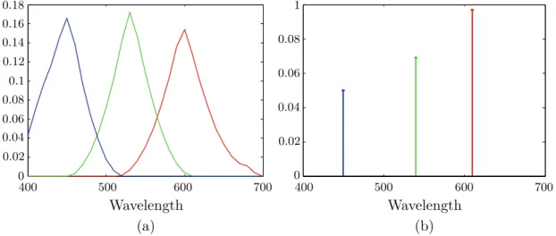
1 (a): Typical RGB camera sensors—Sony DXC930 camera. (b):
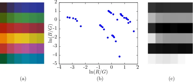
Theo-retical narrowband RGB camera sensors. . . 6 2 (a) The set of 6 patches under different Planckian lights. (b)
Log-chromaticity plot of image (a). (c) The resulting illuminant invariant
image. . . 8 3 Obtaining the 1D shadow invariant image from the band-ratio
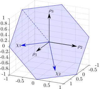
log-chromaticity space. . . 10 4 The plane on which components 𝜌 of geometric mean log chromaticity
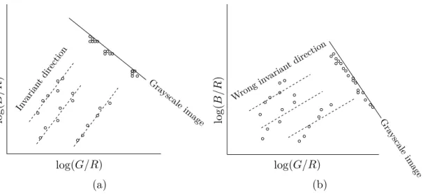
space are placed. . . 10 5 Intuition for finding best direction via minimizing the entropy. (a):
Log-ratio feature space values for paint patches fall along parallel lines, as lighting is changed. Each patch corresponds to a single probability peak when projected in the direction orthogonal to the direction of lighting change. (b): Projecting in the wrong direction leads to a 1D pdf which
is less peaked, and hence of larger entropy. . . 12 6 (a)The difference between entropy plot calculated from image with sky
and from image with sky removed. (b),(c) The grayscale images
cor-responding to minimal entropy if sky wasn’t removed (b) and if sky was removed (c). . . 15 7 The principle of Rayleigh scattering (a)at daylight and(b)at sunset. . 16
8 (a)An example of the image with road. (b)An example of the shadow
free image. . . 20 9 (a)An example of the classification rule result performed on figure 8(b).
(b) An example of the combination of morphological operations used
on (a). . . 21 10 An example of the image with road. . . 26 11 Probability maps of figure 10. (a) Probability of 𝑥 matching a road
model 𝒫𝐺𝑀 𝑀0. (b) Negative log-likelihood of (a) 𝑤𝑝,0,norm. (c) The
illustration of a structural term. (d) Probability of 𝑥 matching a
non-road model 𝒫𝐺𝑀 𝑀1. (e)Negative log-likelihood of (d) 𝑤𝑝,1,norm. . . 28
12 Road detection (based on the illuminant invariance) quality depending on parameters𝑝1 and 𝑝2 in entropy minimization algorithm 1. . . 32
13 Continuous road detection (based on the illuminant invariance) quality depending on parameters𝑝1 and𝑝2 in entropy minimization algorithm 1. 32
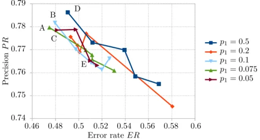
14 The precision and the error rate of road classification rule in illuminant invariance method, depending on the parameter𝑘. . . 35
15 The precision and the error rate of continuous road found using illumi-nant invariance method, depending on the parameter𝑘. . . 35
16 The mobile robot used in my experiments. . . 36 17 A photo of a white sheet of paper made by HD-3000 web camera. . . 37 xv
18 The illustration of the invariant angle estimation on web camera c920.
First row: original images. Second row: entropy plots. Third row:
grayscale images corresponding to the minimal entropy. Fourth row:
grayscale images corresponding to alngle𝜃= 152. . . 38
19 Vectors used to calculate the error value for PID controller. . . 39 20 The results of the illuminant invariance based road detection in
exper-iments with robot. Figure contains 10 evenly distributed images from DS3 and corresponding found paths. . . 39 21 The results of the combined method of road detection in experiments
with robot. Figure contains 10 evenly distributed images from DS3 and corresponding found paths. . . 40 22 The results of the GMM based road detection in experiments with robot.
Figure contains 5 evenly distributed images from DS3 and corresponding found paths. . . 41
List of Tables
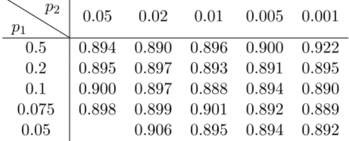
1 Precision of road classification rule based on illuminant invariance, de-pending on parameters𝑝1 and 𝑝2. . . 33
2 Error rate of road classification rule based on illuminant invariance, de-pending on parameters𝑝1 and 𝑝2. . . 33
3 Precision of road detection (continuous) based on illuminant invariance, depending on parameters𝑝1 and𝑝2. . . 33
4 Error rate of road detection (continuous) based on illuminant invariance, depending on parameters𝑝1 and𝑝2. . . 33
5 The precision and the error rate of road classification rule in illuminant invariance method, depending on the parameter𝑘. . . 34
6 The precision and the error rate of continuous road found using illumi-nant invariance method, depending on the parameter𝑘. . . 36
7 The calculated invariant angle𝜃𝐷𝑆2 found in different images. . . 38
8 The content of the attached CD. . . 45
List of algorithms
1 The main principle of the entropy minimization . . . 13 2 The algorithm finding Otsu’s threshold . . . 18 3 The creation of a GMM from the set of pixels . . . 26
Chapter 1
Introduction
One of the most essential robot skills in the field of mobile robotics is to be able to identify driveable area and to be able to stay in it during the movement. To perform this task, robots are equipped with variety of sensors allowing to gain information about the surroundings. Sensors which can be used for road detection include mostly cameras and laser rangefinders. Many researchers focus on visual road detection because cameras are cheap and are able to provide the robot with a lot of useful information. From a single image it’s possible to extract region and boundary features [1]. Region-based features include color, texture and illuminant invariance, while the boundary is defined mostly by road borders and vanishing point. By combining two cameras it’s even possible to use stereo vision to recover depth information [2]. Some studies rely only on one image feature in road detection, while other combine different approaches or utilize information from other sensors [3].
This thesis is focused on the visual path detection in a single image from a single camera. The main approach I’ve taken is to use the illuminant invariance intrinsic property of the image. This method is based on a physical theory of a color image formation. According to the theory, RGB images from narrow-band cameras have a property allowing to construct an illuminant invariant, e.g. shadow free, image. In such image, road area would have a uniform color independent of the light conditions in the original image.
The other approach I implement is a road detection based on the road color. It utilizes Gaussian Mixture Models (GMMs) in order to represent road and non-road color models. The method combines color information with edge detector to compose a graph. The road detection task is therefore transformed into finding this graph’s minimum cut. Furthermore, I implement a combination of both methods in attempt to improve the results.
1.1 Thesis outline
The thesis is composed of 5 chapters. In chapter 1—Introduction—I describe the thesis structure and present state of the art methods of road detection in section 1.2.
In chapter 2 I introduce the theory of the illuminant invariance. I describe how the shadow free image is formed and how the invariant angle parameter is computed. I also describe the sky detection method. Afterwards, I present the methods of road detection in the illuminant invariant image.
In chapter 3 I describe the usage of Gaussian Mixture Models in road detection task, present the road detection technique and propose a combination of GMM method with illuminant invariance algorithms.
In chapter 4 I present performed experiments, explain the parameter estimation and evaluate the results.
Chapter 1 Introduction
1.2 State of the Art in Visual Road Detection
The field of visual road detection is based on the usage of the characteristic road prop-erties presented in images. The most approaches found in science literature are focused on the color or/and structure properties of roads. Various combinations of both ap-proaches are often used to increase robustness of the results.
One of the color-based approaches is to use Gaussian Mixture Models (GMMs), as described in [3]. Authors use GMMs to create the road model and use it co classify pixels in the input image. The update of road model is performed to adapt the model to the changing environment, the approach though uses laser range finder to select pixels for update.
Other example of GMM implementation can be found in [4], where road detection for aerial vehicle is considered. Authors propose an interesting approach of combining road and non-road models created using GMMs with edge detection to find the road using min-cut/max-flow algorithm. Road detection is then combined with homography based road tracking to speed up the overall algorithm.
Another approach was used in [5], where authors use algorithm composed of two modules. First uses intensity image to find candidates to the road boundary. The second module is based on the assumption, that road region color can be described by the multivariate Gaussian distribution. Here, the color information is used to find the road region and reinforce the best matching boundary.
A big area of visual road detection is composed of algorithms based on the illuminant invariance theory. This theory as described in [6] allows to create shadow free grayscale images and even reconstruct colorful shadow free images. In road detection though the grayscale image is sufficient to find road regions and color reconstruction based on given approach is rarely (if ever) used. In [7] authors create grayscale shadow free image using the mentioned approach and find the road areas according to the likelihood-based classifier. In [8] authors also create illuminant invariant image. The road classification is performed by equalization of the grayscale image and subsequent thresholding.
Authors of [2] propose to improve the results of the illuminant invariant image for-mation by ignoring the sky area of the image. Authors also propose another approach to road-nonroad classification based on the use of confidence intervals. To further improve results, algorithm utilizes the stereo-vision allowing to reconstruct the depth information.
Authors of [9] proposed to use image boundary prior to overcome the problems as-sociated with usage of seeds. The assumption was made in many studies that the center-lower part of an image is a road region. In some cases this isn’t necessary true, therefore authors proposed to use another assumption, that the road region has the large common boundary with the bottom part of an image. The color information is used to over-segment the image into several patches. The segmented parts are then classified as road or non-road based on the mentioned assumption. Moreover, the illu-minant invariant grayscale image is embedded into the algorithm to eliminate the effect of shadows.
The approach presented in [10] proposes the method to detect unstructured roads. Authors use texture information at every pixel to detect the vanishing point of the main part of the road. The found vanishing point is then used to estimate two most dominant edges and segment the road.
Different approach is described in [11]. Authors implemented the combination of scene and pixel-based classifiers. The scene classifier uses learned road geometry mod-els to estimate the type of the input image and create a road probability map. The 2
1.2 State of the Art in Visual Road Detection
computed map is then combined with the probability map of the pixel-based classifier to improve the result.
The survey comparing some of the mentioned approaches and more is presented in [1].
Chapter 2
Illuminant invariant images
One of the challenges of an autonomous robotics in the outdoor environment is the detection of the free road space. This task is complicated by various factors, including the variations in the road and background colors and textures, presence of obstacles, illumination conditions. The last is responsible for the appearance of shadows, which create the undesirable color variance on the road surface. Particularly challenging cases are when the road contains both illuminated and shaded regions, as they tend to be classified as different classes. One of the possible approaches to overcome this obstacle is to create an illuminant invariant image and use it to detect the road regions. In this chapter the method to create an illuminant invariant image using the intrinsic features of an RGB image is described.
2.1 RGB image formation
The RGB color is defined as a triple R= (𝑅1, 𝑅2, 𝑅3) = (𝑅, 𝐺, 𝐵). The value of each
component depends not only on actual color of an object, but is also affected by various factors such as shape and reflectance of objects, properties and location of the illuminant and observer [12]. Description of the pixel formation, accounting all these parameters is a complex task. Therefore to make problem simpler, researches use simplified models. The theory of the shadow removal considers, that the world consists of Lambertian surfaces, i.e. surfaces which reflect the light in all directions. This assumption can be used in practice, as many real surfaces are close to Lambertian, as stated in [13]. Under this simplification the pixel formation can be described [6] by the following formula:
𝑅𝑘=𝜎 ∫︁
𝐸(𝜆)𝑆(𝜆)𝑄𝑘(𝜆)d𝜆, 𝑘= 1, 2, 3, (1)
where𝜆is wavelength,𝜎is Lambertian shading. 𝐸(𝜆) is the spectral power distribution
of the illuminant, denoting the amount of power emitted at each wavelength from the interval of the visible spectrum. 𝑆(𝜆) is the surface spectral reflectance function,
defining the amount of the incident light which was reflected from the surface at each wavelength. 𝑄𝑘(𝜆) is the camera sensor sensitivity function, describing the proportion
of the incident light absorbed by the sensor 𝑘 at each wavelength [12, 14].
If the camera sensor sensitivity function is equal to Dirac delta function 𝑄𝑘(𝜆) = 𝑞𝑘𝛿(𝜆−𝜆𝑘), then equation (1) is simplified to:
𝑅𝑘 =𝜎𝐸(𝜆𝑘)𝑆(𝜆𝑘)𝑞𝑘. (2)
In practice, camera sensors aren’t manufactured to be sensitive to one specific wave-length. Typical camera sensor is sensitive to a range of wavelengths with one maximum. The example sensor response is shown in figure 1 (a), where the three sensors, Red, Green and Blue, of Sony DXC930 camera are depicted. Authors of [6] claim, that al-though real sensors aren’t described precisely by Dirac delta function, as in figure 1 (b), 5
Chapter 2 Illuminant invariant images 0 0.18 Wavelength Wavelength 0.16 0.14 0.12 0.1 0.08 0.06 0.04 0.02 0 0.08 0.06 0.04 0.02 1 400 500 600 700 400 500 600 700 (a) (b)
Figure 1 (a): Typical RGB camera sensors—Sony DXC930 camera. (b): Theoretical
narrow-band RGB camera sensors.
From International Journal of Computer Vision, "Entropy Minimization for Shadow Re-moval", Volume 85, Issue 1, p 41, by Graham D. Finlayson, Mark S. Drew, Cheng Lu. ©Springer Science+Business Media, LLC 2009. Reprinted with permission of Springer.
the theory can still be used if sensors are sufficiently narrow-band. Even in case, when sensors are broad-band and described theory doesn’t apply, good results may still be obtained if sensors are appropriately transformed. The possible approach may be spec-tral sharpening proposed in [15]. The goal of this approach is to create new sensor sensitivities by finding a linear combination of the given set of sensors, for which the result is the most narrow-band. Other possible technique is to use sensor transforms deliberately to enhance the resulting invariant image, as proposed in [16].
The next assumption is that the illumination can be described by Planck’s law in Wien’s approximation as in [17]: 𝐸(𝜆, 𝑇)≈ 𝑎1 𝑛2𝜆5𝑒 − 𝑎2 𝑛𝑇 𝜆 = 2𝜋ℎ𝑐 2 0 𝑛2𝜆5 𝑒 −−ℎ𝑐0 𝑛𝑘𝑇 𝜆 W/m2, (3)
where 𝑎1 ≈3.742×10⁻¹⁶ Wm2 and 𝑎2 ≈1.439×10⁻² mK are constants, ℎ is Planck
constant,𝑘is Boltzmann constant,𝑐0 is the speed of light in vacuum. 𝑛is the refractive
index,𝑇 is the temperature of a black-body radiator in Kelvins. Since𝑛= 1.0001 in air,
it can be omitted. The Wien’s approximation can be used if𝑒(𝑎2/(𝑛𝜆𝑇))≫1. According
to [18], temperatures up to𝑇 = 10000𝐾 can be expected in real applications, and the
visible spectrum consists of wavelengths in range from 400 to 700 nm. Therefore, the minimum expected value is 𝑒(𝑎2/(𝑛𝜆𝑇)) ≈7.810 and the Wien’s approximation can be
used. The authors have also compared Planck’s equation and the Wien’s approximation of several black-body radiants expected in real-life applications, claiming the results are similar.
Equation (3) describes shapes of the power distribution, but doesn’t take into ac-count illuminant power. Therefore the light intensity constant 𝐼 is added to Wien’s
approximation to model varying power:
𝐸(𝜆, 𝑇)≈𝐼𝑎1𝜆−5𝑒−
𝑎2
𝑇 𝜆. (4)
After substituting equation (4) into equation (1), components of the RGB color R
are given as:
𝑅𝑘 =𝜎𝐼𝑎1𝜆−𝑘5𝑒 (︁ − 𝑎2 𝑇 𝜆𝑘 )︁ 𝑆(𝜆𝑘)𝑞𝑘, 𝑘= 1, 2, 3, (5) 6
2.2 Chromaticity space
2.2 Chromaticity space
The chromaticity is a color specification, that isn’t dependent on its luminance [6], i.e. "quotient of the luminous intensity and the projected area of the source in a given direction" as defined in [14]. According to the same source, this quantity "correlates with perceived brightness". In chromaticity specification individual pixels lose infor-mation about their luminance. But that doesn’t mean, that such image is shadow free, because luminance isn’t the only parameter, which affects shadow formation. As stated in [6], the difference between non-shadowed and shadowed regions isn’t that ones are illuminated and others aren’t. In most cases they both are illuminated, but by different sources. For example, at daylight shadow is illuminated by sky only, while non-shadowed areas by both sky and sun. These two illuminants have different temper-atures, which also affect pixel formation, according to equation (5). Since temperature information can still be present in chromaticity space, shadows don’t disappear.
The chromaticity is defined in such a way, that many different descriptors can comply with it. In this section three of them are described, namely, L1 norm, Band-ratio log
chromaticity and Geometric mean log chromaticity.
L1 norm
One of the most known chromaticity spaces is defined using the L1 norm. Components
r of this space are created by normalizing components of a RGB pixelR according to
the formula: r= (𝑟1, 𝑟2, 𝑟3) = (𝑟, 𝑔, 𝑏) = (︂ 𝑅 1 𝑅1+𝑅2+𝑅3 , 𝑅2 𝑅1+𝑅2+𝑅3 , 𝑅3 𝑅1+𝑅2+𝑅3 )︂ . (6)
As emerged from the equation (5), the light intensity𝐼 and the Lambertian shading 𝜎 are canceled out in each component ofr:
𝑟𝑘= 𝜎𝐼𝑎1𝜆−𝑘5𝑒 (︁ − 𝑎2 𝑇 𝜆𝑘 )︁ 𝑆(𝜆𝑘)𝑞𝑘 𝜎𝐼𝑎1∑︀3𝑖=1 (︃ 𝜆−𝑖 5𝑒 (︁ − 𝑎2 𝑇 𝜆𝑖 )︁ 𝑆(𝜆𝑖)𝑞𝑖 )︃, 𝑘= 1,2,3. (7)
The image formed by ris thus intensity free. Unfortunately, shadows are not removed
by this simple operation, as luminant-dependent parameter (temperature 𝑇) is present
in equation (7). L1 norm removes luminance, but due to its properties, it’s not
use-ful in illuminant invariance image formation, although it’s still used in color recovery algorithms.
Band-ratio log chromaticity
Contrarily, band-ratio and geometric mean log chromaticity are defined in such a way, that they can be used in shadow removal task. The band-ratio chromaticity space is defined by obtaining band-ratios 𝑐= (𝑐1, 𝑐2) as:
𝑐𝑘= 𝑅𝑘 𝑅𝑝
, (8)
where 𝑝 is one of the channels 𝑝 ∈ {1,2,3} and 𝑘 = 1,2 indexes the remaining two
channels .
Chapter 2 Illuminant invariant images -5 -4 -3 -2 -1 0 1 2 -4 -3 -2 -1 0 1 2 ln ( 𝐵 /𝐺 ) ln(𝑅/𝐺) (a) (b) (c)
Figure 2 (a)The set of 6 patches under different Planckian lights. (b)Log-chromaticity plot
of image (a). (c)The resulting illuminant invariant image.
The created chromaticity space is free of intensity and Lambertian shading infor-mation, since according to the equations (8) and (5), corresponding components are canceled out: 𝑐𝑘= 𝑅𝑘 𝑅𝑝 = 𝑎1𝜆−𝑘5𝑆(𝜆𝑘)𝑞𝑘𝑒 (︁ − 𝑎2 𝑇 𝜆𝑘 )︁ 𝑎1𝜆−𝑝5𝑆(𝜆𝑝)𝑞𝑝𝑒 (︁ − 𝑎2 𝑇 𝜆𝑝 )︁. (9)
The band-ratio log chromaticity space𝜌= (𝜌1, 𝜌2) is obtained by taking the logarithm
of 𝑐. The components of this chromaticity space have a form 𝜌𝑘= log (𝑐𝑘) = log (︃ 𝑠𝑘 𝑠𝑝 )︃ + log (︃ 𝑒(𝑒𝑘/𝑇) 𝑒(𝑒𝑝/𝑇) )︃ = log (︃ 𝑠𝑘 𝑠𝑝 )︃ +𝑒𝑘−𝑒𝑝 𝑇 , (10)
where 𝑠𝑘,𝑝 = 𝑎1𝜆−𝑘,𝑝5𝑆(𝜆𝑘,𝑝)𝑞𝑘,𝑝 and 𝑒𝑘,𝑝 = −𝑎2/𝜆𝑘,𝑝. Evidently, this space is still
luminance-free.
The illuminant invariant space can be obtained by extracting the last luminant-dependent parameter 𝑇 from definition (10) of 𝜌1 and substituting it to the 𝜌2, giving
𝜌2= log (︃ 𝑠2 𝑠𝑝 )︃ −𝑒2−𝑒𝑝 𝑒1−𝑒𝑝log (︃ 𝑠1 𝑠𝑝 )︃ +𝑒2−𝑒𝑝 𝑒1−𝑒𝑝 𝜌1. (11)
This equation shows, that projections of pixels to the band-ratio log-chromaticity space form parallel lines with the same slope. The offsets are dependent on surfaces. The individual points on the same line represent the difference in the illumination and shading, according to [7].
The example of how the log-chromaticity plot is formed is shown in figure 2. In figure (a) the set of 6 patches from the Macbeth color checker is shown under 6 different Planckian lights in a range from 2500 K to 10000 K. Figure (b) shows where these patches are projected in the log-chromaticity plot. Here, the straight lines formed due to the change of the illuminant can be seen. In figure (c) the resulting illuminant invariant image is shown.
The illuminant invariant image can be obtained by projecting points of the band-ratio log-chomaticity space onto the direction v⊥ perpendicular to the vector v =
(𝑒2−𝑒𝑝, 𝑒1−𝑒𝑝)𝑇. From the resulting set of scalars the grayscale shadow invariant
image can be produced. 8
2.3 Obtaining the grayscale shadow invariant image
Geometric mean log chromaticity
The band-ratio log chromaticity can be used to create shadow invariant images. But it’s necessary to choose, which channel should be used as a divisor. If an image happens to have all pixels with small red values and the red channel is chosen as a divisor, then outliers may occur. Various light conditions such as bright sun, clouds or shadows may result in different colors to be more or less intense. Additionally if the camera’s color balance isn’t properly set, then it may happen that some of the channels lack intensity. In the changing environment it’s hard to predict what light conditions can be expected and how would they affect the color balance. The possible method to overcome these limitations is to divide by the geometric mean of all channels, instead of preferring one of them. Such divisor increases the robustness to noise [19], as the small value in one of the channels can be compensated by the remaining channels, effectively reducing the number of the outliers.
The geometric mean chromaticity space is created using vectors𝑐= (𝑐1, 𝑐2, 𝑐3), where
the components are
𝑐𝑘= 𝑅𝑘 3 √ 𝑅1𝑅2𝑅3 , (12)
and 𝑘= 1,2,3. Such definition ofc is the chromaticity, since the intensity and shading
information are canceled out:
𝑐𝑘= 𝜎𝐼𝑎1𝜆−𝑘5exp (︁ − 𝑎2 𝑇 𝜆𝑘 )︁ 𝑆(𝜆𝑘)𝑞𝑘 𝜎𝐼𝑎1 3 ⎯ ⎸ ⎸ ⎷∏︀3𝑖 =1 (︃ 𝜆−𝑖 5𝑒 (︁ −𝑎2 𝑇 𝜆𝑖 )︁ 𝑆(𝜆𝑖)𝑞𝑖 )︃ , (13) where 𝑘= 1,2,3.
The geometric mean log chromaticity space is derived from 𝑐 by taking the natural
logarithm of individual components
𝜌𝑘 = ln (𝑐𝑘) = ln ⎛ ⎝ 𝑠𝑘 3 √︁ ∏︀3 𝑖=1𝑠𝑖 ⎞ ⎠+ 1 𝑇 (︃ 𝑒𝑘−13 3 ∑︁ 𝑖=1 𝑒𝑖 )︃ = ln(︂𝑠𝑘 𝑠𝑚 )︂ +𝑒𝑘−𝑒𝑚 𝑇 , (14)
where 𝑠𝑘,𝑖 = 𝑎1𝜆−𝑘,𝑖5𝑆(𝜆𝑘,𝑖)𝑞𝑘,𝑖 and 𝑒𝑘,𝑖 = −𝑎2/𝜆𝑘,𝑖. This equation looks similar to
the equation (10). However, the pixel from geometric mean log chromaticity space is composed from three components, not two. To obtain the illuminant invariant image from this space, additional computations presented in the next section are necessary.
2.3 Obtaining the grayscale shadow invariant image
Due to the property of the band-ratio log-chromaticity space to form straight lines from the RGB pixels formed on the same surface, it can be used to create shadow free images. As will be shown below, the geometric mean log chromaticity space can be transformed to have similar properties.
Band-ratio log chromaticity space
The situation described by the equation (11) is depicted in the figure 3. The individual points in the log-log plot form parallel lines. The slope is dependent only on the camera parameters and is defined by vector v = (𝑒2−𝑒𝑝, 𝑒1−𝑒𝑝)𝑇. The offset is dependent
Chapter 2 Illuminant invariant images log(𝑅/𝐺) log(𝐵/𝐺) 𝜃 ⃗ 𝑣 0 ℐ𝜌 ⃗𝑣⊥ 𝜌1 𝜌2
Figure 3 Obtaining the 1D shadow invariant image from the band-ratio log-chromaticity space.
-1 -0.5 0 0.5 1 1 0.5 0 -0.5 -1 -0.4 -0.20 0.2 0.4 0.6 0.81 -0.6 -1 -0.8 𝜌1 𝜌2 𝜌3 𝜒1 𝜒2
Figure 4 The plane on which components 𝜌 of geometric mean log chromaticity space are
placed.
on the surface, but not on the shading, illumination nor temperature. Thus projecting points on the linev⊥perpendicular to the vectorvloses the shading information, while
still distinguish individual surfaces. The slope of the line v⊥ is given by the camera
dependent parameter called illuminant-invariant angle𝜃 [7]. With such definition of𝜃,
the projection of the point 𝜌 = (𝜌1, 𝜌2) onto the line v⊥ can be calculated using the
formula
ℐ𝜌=𝜌1cos (𝜃) +𝜌2sin (𝜃). (15)
The angle 𝜃 isn’t known and has to be correctly estimated, so that the resulting
grayscale image is shadow free. The methods to find the illuminant-invariant angle are described in section 2.4.
Geometric mean log chromaticity space
Unlike the previous case, the geometric mean log chromaticity pixels are composed of three components. In this case the grayscale image is obtained by firstly projecting from the 3D space onto a 2D and then to 1D.
The points𝜌= (𝜌1, 𝜌2, 𝜌3) aren’t independent [6]. In fact, for each pixel, the
calcu-lated geometric mean log chromaticity is placed on the plane 𝑢⊥ depicted in figure 4.
2.4 Obtaining the illuminant-invariant angle
This plane is constrained by equation
𝜌1+𝜌2+𝜌3 = ln (︂ 𝑅 1 3 √ 𝑅1𝑅2𝑅3 )︂ + ln(︂ 𝑅2 3 √ 𝑅1𝑅2𝑅3 )︂ + ln(︂ 𝑅3 3 √ 𝑅1𝑅2𝑅3 )︂ = ln(︂𝑅1𝑅2𝑅3 𝑅1𝑅2𝑅3 )︂ = ln (1) = 0, (16)
and is perpendicular to the vector 𝑢= √1
3(1,1,1)
𝑇, since𝜌·𝑢= 0.
To characterize the 2D space, the projector𝑃𝑢⊥onto this plane is considered [6]. The
projection of 𝜌 onto a vector 𝑢 is defined by a projection matrix 𝑃𝑢 = 𝑢𝑢
𝑇
𝑢𝑇𝑢 = 𝑢𝑢𝑇, according to [20]. The projection of 𝜌 onto a space orthogonal to 𝑢is 𝑃𝑢⊥=𝐼−𝑃𝑢 = 𝐼−𝑢𝑢𝑇, where𝐼 is the identity matrix. On the other hand, the projection matrix can
be decomposed as 𝑃𝑢⊥ = 𝑈𝑇𝑈, where 𝑈 is the 2×3 matrix with orthonormal rows.
Defined this way, matrix 𝑈 is used to transform points𝜌 into the coordinate system𝜒
on the plane 𝑢⊥:
𝜒= (𝜒1, 𝜒2)𝑇 =𝑈𝜌. (17)
The matrix𝑈 can be composed in any way so that𝑈𝑇𝑈 =𝐼−𝑢𝑢𝑇 and the conditions
above hold true. The value proposed in [6] is used in this thesis:
𝑈 = [︃√1 2 − 1 √ 2 0 1 √ 6 1 √ 6 − 2 √ 6 ]︃ . (18)
Deriving from the equations (14) and (17), individual points in the discussed 2D space 𝜒have coordinates
𝜒1= √1 2 (︂ ln(︂𝑠1 𝑠𝑚 )︂ +𝑒1−𝑒𝑚 𝑇 )︂ −√1 2 (︂ ln(︂𝑠2 𝑠𝑚 )︂ +𝑒2−𝑒𝑚 𝑇 )︂ = √1 2ln (︂𝑠 1 𝑠2 )︂ +√1 2 𝑒1−𝑒2 𝑇 𝜒2= √1 6ln (︂𝑠 1𝑠2 𝑠2 3 )︂ +√1 6 𝑒1+𝑒2−2𝑒3 𝑇 . (19)
The equations above have similar properties to the equation (10). Similarly to the equation (11) points 𝜒= (𝜒1, 𝜒2) form parallel lines with slope dependent only on the
camera parameters and offsets dependent on the surfaces:
𝜒2 = √1 2ln (︂𝑠 1𝑠2 𝑠3 )︂ −√1 6 𝑒1+𝑒2−2𝑒3 𝑒1−𝑒2 (︂𝑠 1 𝑠2 )︂ +√1 3 𝑒1+𝑒2−2𝑒3 𝑒1−𝑒2 𝜒1. (20)
Obtaining of the grayscale image is similar to the situation in the band-ratio log chro-maticity space, shown in the figure 3. The projection of points (𝜒1, 𝜒2) onto the 1D
space is calculated using the equation (15), where 𝜌=𝜒.
2.4 Obtaining the illuminant-invariant angle
Knowing the correct illuminant-invariant angle 𝜃 is essential to the creation of the
shadow free image. If 𝜃 isn’t correct, then the situation depicted in figure 5 can
oc-cur. In figure 5(a) 𝜃 is correctly estimated. Here, shading, illumination and luminant
temperature are removed, since the points forming one line have similar value in the 1D space. In figure 5(b) the illuminant-invariant direction isn’t correctly found, which 11
Chapter 2 Illuminant invariant images Gra yscale image Gra ysc ale image Invarian tdirection Wrong invarian t direction log(𝐺/𝑅) log(𝐺/𝑅) log ( 𝐵 /𝑅 ) log ( 𝐵 /𝑅 ) (a) (b)
Figure 5 Intuition for finding best direction via minimizing the entropy. (a): Log-ratio feature
space values for paint patches fall along parallel lines, as lighting is changed. Each patch corresponds to a single probability peak when projected in the direction orthogonal to the direction of lighting change. (b): Projecting in the wrong direction leads to a 1D pdf which
is less peaked, and hence of larger entropy.
From International Journal of Computer Vision, "Entropy Minimization for Shadow Re-moval", Volume 85, Issue 1, p 37, by Graham D. Finlayson, Mark S. Drew, Cheng Lu. ©Springer Science+Business Media, LLC 2009. Reprinted with permission of Springer.
causes, that points with different illumination are projected onto different values in 1D space, causing shadows to appear in the grayscale image.
Several methods to estimate𝜃 are used in the literature. These methods are mostly
based on the two approaches—camera calibration and entropy minimization.
The camera calibration method is described in [6]. It’s based on the idea, that since the illuminant-invariant angle is dependent only on the camera parameters, it can be estimated off-line. This method requires to perform a calibration using the camera, can’t be used on the single image made by unknown camera and isn’t robust to changes. Therefore methods based on the entropy minimization were proposed. These meth-ods’ main idea is that the grayscale image calculated with the correct value 𝜃 will
have smaller entropy, than images calculated with wrong value of 𝜃. The best
esti-mation of 𝜃 is found by comparing grayscale images generated with different angles.
In [6] two methods—entropy minimization and information potential maximization— were described. The authors of [8] use entropy minimization, but differ in the detection of outliers. Authors of [21] also use entropy minimization, but adopt different to [6] and [8] rule for histogram bin width calculation. Authors of [7] use entropy minimiza-tion, but propose another way to determine outliers and claim to find more stable results of 𝜃 by minimizing the average entropy distribution of a set of input images
instead of using the single image. 2.4.1 Entropy Minimization
The main principle of entropy minimization is described in algorithm 1. The illuminant invariant direction is found by comparing entropies of grayscale images corresponding to all possible angles. Firstly, the 2D log-chromaticity space is computed for the given image. Then, for each angle 𝜃= {1, . . . ,180}, the 1D illuminant invariant image ℐ is
computed. After careful outlier detection the entropy is calculated. The angle corre-sponding to the minimal entropy is chosen as the correct illuminant-invariant angle. 12
2.4 Obtaining the illuminant-invariant angle
Algorithm 1:The main principle of the entropy minimization Input : RGB image
Output: Grayscale image corresponding to𝜃 with minimal entropy
1 Create 2D log-chromaticity image 𝜒 2 𝑚𝑖𝑛𝐸𝑛𝑡𝑟𝑜𝑝𝑦=∞
3 𝑚𝑖𝑛𝑇 ℎ𝑒𝑡𝑎= 0 4 for𝜃= 1. . .180do
5 Compute illuminant invariant image ℐ from 𝜒with angle𝜃 6 Choose inliers from ℐ
7 Calculate the appropriate histogram bin width 8 Create histogram from inliers
9 Calculate entropy𝑒𝑛𝑡𝑟𝑜𝑝𝑦 from histogram 10 if 𝑒𝑛𝑡𝑟𝑜𝑝𝑦 < 𝑚𝑖𝑛𝐸𝑛𝑡𝑟𝑜𝑝𝑦then
11 𝑚𝑖𝑛𝐸𝑛𝑡𝑟𝑜𝑝𝑦 =𝑒𝑛𝑡𝑟𝑜𝑝𝑦 12 𝑚𝑖𝑛𝑇 ℎ𝑒𝑡𝑎 =𝜃
13 Compute illuminant invariant image ℐ from 𝜒with angle𝑚𝑖𝑛𝑇 ℎ𝑒𝑡𝑎
In entropy minimization algorithm the comparison of different grayscale images is done with Shannon entropy
𝜂= 𝑛 ∑︁ 𝑖=1
−𝑝𝑖lb𝑝𝑖, (21)
where𝑛is the number of histogram bins,𝑝𝑖is the probability of the bin and lb denotes
the binary logarithm. However, such definition of entropy is sensitive to the choice of the histogram bin width. If the bin width is too small, then algorithm is prune to noise. On the contrary, if the bin width is too big, then the precision is lost. The bad choice can lead images with different values and standard deviations to not being treated equally and the wrong imageℐ𝜃to be favored. Therefore, methods, which adapt
bin width to the individual image, are used in many studies.
In the illuminant invariance theory the most used formula to compute the appropriate bin width ℎ is Scott’s normal reference rule for normally distributed data:
ℎ= 3.5𝜎
𝑁1/3, (22)
where 𝑁 is the number of inliers and 𝜎 is their standard deviation. Implementation of
this rule needs careful detection of outliers. I implement this rule in my algorithm. The other possibility is to use Freedman and Diaconis’ bin width, as proposed in [21]:
ℎ= 2 IQR
𝑁1/3 , (23)
where 𝑁 is the number of samples and IQR is the interquartile range. The above
equation can be more robust, than Scott’s reference rule, as IQR is less sensitive to the outliers.
2.4.2 Outlier detection
Scott’s normal reference rule for bin width calculation assumes normally distributed data, which makes it sensitive to outliers. Often outliers are pixels with very small or large value of 𝑅, 𝐺 and/or 𝐵. Such pixels correspond to infinite or very big numbers
Chapter 2 Illuminant invariant images
in log chromaticity spaces. If not deleted from computations these pixels contribute to calculations of mean and standard deviation. The resulting mean may shift from the position dictated by inliers. The standard deviation may be bigger, making histogram bin width to lose precision.
In literature different methods of outlier detection are presented. Finlayson, Drew and Lu in [6] implement a simple rule to differentiate between inliers and outliers. They propose to use only middle 90% of all pixels to create a histogram. This method assumes that outliers are presented only in 5% of the lowest and 5% of the biggest values. The problem with this method is that if the number of actual outliers is much bigger than 10% it can still be prone to errors.
Another approach is used by Krajník, Blažíček and Santos in [8]. Authors also use a simple rule: values 𝑖 which are lower than one threshold 𝑖𝑚𝑖𝑛 or bigger than the
other 𝑖𝑚𝑎𝑥 are called outliers. Authors use values 𝑖𝑚𝑖𝑛 = 0.05 and 𝑖𝑚𝑎𝑥 = 0.95 for
normalized image. Note, that unlike the previous method the number of inliers is variable between different histograms. This method solves the issue of the big number of outliers. Although, it may have troubles adapting to histograms, where inliers are shifted to one of the sides. It may not be the problem, if the shift is expected to be the same in all of the images. Unfortunately, in my application it’s not the case—inliers change their values from dark to light depending on the invariant angle.
Alternatively, in [7] Álvarez and López proposed a method, which addresses both of the issues. They utilize the algorithm capable of adapting to the unique range of values of each image. The algorithm is presented in detail in [22]. It’s based on the Chebyshev’s inequality in a form:
𝑃(|𝑋−𝜇| ≥𝑘𝜎)≤ (︂ 1
𝑘2
)︂
, (24)
where 𝑋 represents the random variable, 𝜇 is the expected or mean value, 𝜎 is the
standard deviation and 𝑘 is the number of standard deviations from the mean. The
equation shows that less than 1
𝑘2 of data lies further than 𝑘 standard deviations from
the mean 𝜇. Chebyshev’s inequality assumes that data distribution isn’t known, so
authors propose two methods—to work with unknown distribution and an extension of the algorithm to work with unimodal data. In my algorithm I don’t use the unimodal assumption, since pixel of grayscale image may gain various values depending on the original color R and where this color is projected onto the 1D space by invariant angle
𝜃. In outdoors applications colors R presented in the image are unpredictable. If the
distribution happens to be unimodal, algorithm will still work, but the results wouldn’t be as precise as if dedicated algorithm was used.
The goal of the algorithm is to find an Outlier Detection Value𝑂𝐷𝑉. It distinguishes
between the upper value 𝑂𝐷𝑉𝑈 and lover value 𝑂𝐷𝑉𝐿, bounding the distribution.
Every value 𝑖within the boundaries𝑂𝐷𝑉𝐿≤𝑖≤𝑂𝐷𝑉𝑈 is an inlier, everything else is
an outlier.
The calculation of𝑂𝐷𝑉 is divided into two stages. The first stage roughly estimates 𝑂𝐷𝑉 and determines which values aren’t outliers and should be used in calculations in
next step. In the second stage these values are used to more accurately calculate final
𝑂𝐷𝑉.
The first stage is divided into several steps:
1. Decide the probability𝑝1of pixel being a potential outlier. It is a rough estimation
and authors recommend it to be bigger than the expected probability of pixel being an outlier. Authors propose values similar to 𝑝1 ={0.1,0.05,0.01}in this stage.
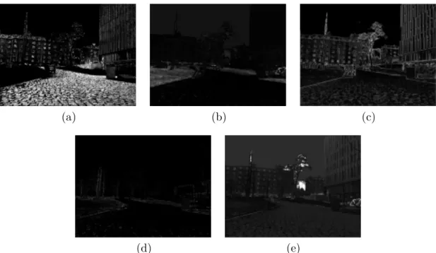
2.5 Sky detection 5 5.1 5.2 5.3 5.4 5.5 5.6 5.7 5.8 5.9 0 20 40 60 80 100 120 140 160 180 En trop y 𝜃
Sky not removed Sky removed
(a) (b) (c)
Figure 6 (a) The difference between entropy plot calculated from image with sky and from
image with sky removed. (b),(c)The grayscale images corresponding to minimal entropy if
sky wasn’t removed (b) and if sky was removed (c).
2. Calculate 𝑘from equation (24):
𝑘= √1
𝑝1 (25)
3. Use the histogramℋ𝜃 to calculate𝜇and 𝜎.
4. Calculate 𝑂𝐷𝑉 from equation (24):
𝑂𝐷𝑉1𝑈 = 𝜇+𝑘𝜎 𝑂𝐷𝑉1𝐿= 𝜇−𝑘𝜎
(26) 5. Create ℋ𝜃2 from values inℋ𝜃 within bounds of 𝑂𝐷𝑉1𝑈 and𝑂𝐷𝑉1𝐿
The second stage is similar to the first stage. It repeats operations from the first stage, but computations are made with other values:
1. Decide the expected probability𝑝2 of pixel being an outlier. Authors recommend
values like 𝑝2 ={0.01,0.001,0.0001}in this stage.
2. Calculate 𝑘from equation (24):
𝑘= √1
𝑝2 (27)
3. Use the histogramℋ𝜃2 to calculate𝜇and 𝜎.
4. Calculate 𝑂𝐷𝑉 from equation (24):
𝑂𝐷𝑉𝑈 =𝜇+𝑘𝜎 𝑂𝐷𝑉𝐿=𝜇−𝑘𝜎
(28) Values 𝑂𝐷𝑉𝑈 and𝑂𝐷𝑉𝐿are the final result of the algorithm. They are used on the
original histogram ℋ𝜃 for distinguishing between inliers and outliers.
2.5 Sky detection
Experiments have shown, that though entropy minimization algorithms are generally good in finding the right invariant angle, they may (often) fail in images with large sky area. The example is shown in figure 6 (b), where invariant angle is incorrectly computed resulting in shadows still be visible in grayscale image. According to [2] 15
Chapter 2 Illuminant invariant images
(a) (b)
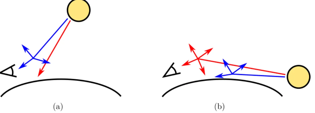
Figure 7 The principle of Rayleigh scattering(a)at daylight and(b)at sunset.
the reason for these errors can be Rayleigh scattering. This phenomenon is a scatter-ing of electromagnetic radiation by particles with dimensions smaller than radiation wavelength [23]. The light is scattered by Earth atmosphere according to formula:
𝐼(𝜆)𝑠𝑐 ∝ 𝐼(𝜆)𝑖𝑛𝑐
𝜆4 , (29)
where𝐼(𝜆)𝑠𝑐is the intensity of the scattered light,𝐼(𝜆)𝑖𝑛𝑐is the intensity of the incident
light and 𝜆is the light wavelength.
According to this formula, the scattering of the light is dependent on the wavelength. Colors with smaller wavelengths (e.g. blue) are scattered more strongly than ones with bigger wavelengths (e.g. red). Due to Rayleigh scattering individual colors in the white light traveling through the atmosphere are not diffused equally. The intuition for this phenomenon is shown in figure 7. During daylight the blue color is scattered in the atmosphere, while red color travels further, as is shown in figure 7(a). The scattered blue light reaches the observer making the sky appear blue. At sunset the distance from the sun to the observer is bigger. The blue color is (almost entirely) scattered away before light reaches the observer, as is shown in figure 7(b). The remaining red light is scattered in the atmosphere from where it reaches the observer making sky appear redder.
Rayleigh scattering also causes the color hue across the sky area, which creates the obstacle for entropy minimization algorithms. In figure 6(a) the minimal entropy cor-responds to the grayscale image (b) with the lowest sky color hue. Contrary, if the sky area was found and removed from computations, the invariant angle was found correctly, as in figure 6(c).
In this thesis an algorithm [24] based on Otsu’s thresholding method [25] is used for horizon and sky detection.
2.5.1 Otsu’s threshold method
The Otsu’s Global thresholding method for gray-level histograms is based on the com-parison of how each gray level performs as a threshold. The algorithm successively chooses each gray-level to divide the histogram into two classes: background and fore-ground. The gray-level minimizing the intra-class variance is then chosen as an optimal threshold. Since sky is generally brighter than the rest of an image, this segmentation method may be safely used to its identification.
Assume a grayscale image with N intensity levels. Otsu’s threshold method uses its normalized gray-level histogram. In such histogram each bin represents the probability 16
2.5 Sky detection
𝑝𝑖 of the corresponding gray-level, 𝑖 = {0,1, . . . , 𝑁 −1}. Each possible threshold 𝑇
divides the histogram into two classes𝐶1 ={0,1, . . . , 𝑇}and𝐶2 ={𝑇+1, 𝑇+2, . . . , 𝑁−
1}.
The class probabilities are
𝑞1(𝑇) = 𝑇 ∑︁ 𝑖=0 𝑝𝑖 and 𝑞2(𝑇) = 𝑁−1 ∑︁ 𝑖=𝑇+1 𝑝𝑖. (30)
The class means are calculated as
𝜇1(𝑇) = 𝑇 ∑︁ 𝑖=0 𝑖𝑃(𝑖|𝐶1) = 𝑇 ∑︁ 𝑖=0 𝑖 𝑝𝑖 𝑞1(𝑇) and 𝜇2(𝑇) = 𝑁−1 ∑︁ 𝑖=𝑇+1 𝑖𝑃(𝑖|𝐶2) = 𝑁−1 ∑︁ 𝑖=𝑇+1 𝑖 𝑝𝑖 𝑞2(𝑇) , (31)
where 𝑃(𝑖|𝐶𝑗) is the conditional probability of gray-level𝑖given class 𝐶𝑗.
The class variance is defined as
𝜎12(𝑇) = 𝑇 ∑︁ 𝑖=0 [𝑖−𝜇1]2𝑃(𝑖|𝐶1) = 𝑇 ∑︁ 𝑖=0 [𝑖−𝜇1]2 𝑝𝑖 𝑞1(𝑇) and 𝜎22(𝑇) = 𝑁−1 ∑︁ 𝑖=𝑇+1 [𝑖−𝜇2]2𝑃(𝑖|𝐶2) = 𝑁−1 ∑︁ 𝑖=𝑇+1 [𝑖−𝜇2]2 𝑝𝑖 𝑞2(𝑇) . (32)
The optimal threshold 𝑇𝑜 is found according to [24] by minimizing the intra-class
(within-class) variance: 𝜎𝑊2 (𝑇𝑜) = min 0≤𝑇 <𝑁𝜎 2 𝑊(𝑇), (33) where 𝜎2𝑊(𝑇) =𝑞1(𝑇)𝜎12(𝑇) +𝑞2(𝑇)𝜎22(𝑇). (34)
Performing all of these operations for every possible threshold𝑇 would be ineffective,
therefore I implemented the method using algorithm 2. Here, the number of compu-tations is minimized by taking variables out of cycle in order to get rid of inner sums. In the following calculations parameter 𝑇 is omitted even though variables are still
dependent on it. Assume, 𝑘= 1,2 stands for each class. Variables 𝑞𝑘,𝜇𝑘 and 𝜎𝑘 aren’t
calculated from the beginning in every iteration for different 𝑇. Instead, new variables 𝜇′𝑘 and𝜎′𝑘are introduced. These variables, as well as𝑞𝑘, are set to zero for𝑘= 1 and to
a maximum value for𝑘= 2. During iterations through gray-levels, variables with𝑘= 1
are increased and variables with 𝑘 = 2 are decreased according to 𝑇. The intra-class
variance 𝜎𝑊2 calculation is changed with respect to new variables.
My calculations start on equations (34) and (32). Since 𝑞𝑘(𝑇) is canceled out, new
variable 𝜎2′′=𝑞𝑘(𝑇)𝜎𝑘2(𝑇) is introduced so that 𝜎𝑊2 =𝜎′′1 +𝜎2′′. It’s equal to
𝜎′′𝑘= ∑︁ 𝑖∈𝐶𝑘 [𝑖−𝜇𝑘]2𝑝𝑖= ∑︁ 𝑖∈𝐶𝑘 [︁ 𝑖2𝑝𝑖−2𝑖𝜇𝑘𝑝𝑖+𝜇2𝑘𝑝𝑖 ]︁ . (35)
Some parameters in this equation aren’t dependent on 𝑖, therefore it can be further
modified: 𝜎′′𝑘= ∑︁ 𝑖∈𝐶𝑘 [︁ 𝑖2𝑝𝑖 ]︁ −2𝜇𝑘 ∑︁ 𝑖∈𝐶𝑘 [𝑖𝑝𝑖] +𝜇2𝑘 ∑︁ 𝑖∈𝐶𝑘 [𝑝𝑖]. (36) 17
Chapter 2 Illuminant invariant images
Algorithm 2:The algorithm finding Otsu’s threshold Input : Normalized histogramℋ𝜃 with𝑁 gray-levels
Output: Otsu’s threshold𝑇𝑜
1 𝜎𝑊2 (𝑇𝑜) =∞ 2 𝑇𝑜 = 0 3 𝑞1 = 0.0,𝑞2 = 1.0 4 𝜇′1=𝜇′2= 0.0 5 𝜎1′ =𝜎′2= 0.0 6 for𝑖= 0. . . 𝑁−1 do 7 𝜇′2=𝜇′2+𝑖·𝑝𝑖 8 𝜎2′ =𝜎′2+𝑖·𝑖·𝑝𝑖 9 for𝑖= 0. . . 𝑁−1 do 10 𝑞1 =𝑞1+𝑝𝑖 11 𝑞2 =𝑞2−𝑝𝑖 12 𝜇′1=𝜇′1+𝑖·𝑝𝑖 13 𝜇′2=𝜇′2−𝑖·𝑝𝑖 14 𝜎1′ =𝜎′1+𝑖·𝑖·𝑝𝑖 15 𝜎2′ =𝜎′2−𝑖·𝑖·𝑝𝑖 16 𝜎1′′=𝜎′1− (𝜇 ′ 1)2 𝑞1 17 𝜎2′′=𝜎′1− (𝜇 ′ 2)2 𝑞2 18 𝜎𝑊2 =𝜎1′′+𝜎′′2 19 if 𝜎2𝑊 <𝜎2𝑊(𝑇𝑜) then 20 𝜎𝑊2 (𝑇𝑜) =𝜎𝑊2 21 𝑇𝑜 =𝑖 According to equation (30), ∑︀
𝑖∈𝐶𝑘[𝑝𝑖] =𝑞𝑘. In order to get rid of the two remaining sums, I define 𝜇′𝑘= ∑︁ 𝑖∈𝐶𝑘 [𝑖𝑝𝑖] and (37) 𝜎′𝑘= ∑︁ 𝑖∈𝐶𝑘 [︁ 𝑖2𝑝𝑖 ]︁ . (38)
Equation (31) can be then rewritten as 𝜇𝑘 = 𝜇′𝑘
𝑞𝑘. Therefore, equation (36), can be further modified: 𝜎𝑘′′=𝜎𝑘′ −2𝜇 ′ 𝑘 𝑞𝑘 𝜇′𝑘+ (︂𝜇′ 𝑘 𝑞𝑘 )︂2 𝑞𝑘=𝜎𝑘′ − (𝜇′𝑘)2 𝑞𝑘 . (39)
All of the described above calculations were made to get rid of the sums inside of iteration through gray-levels. All of the variables present in equation (39) can be declared outside of the cycle and modified at the beginning of every iteration. Number of gray-levels is increasing by one in 𝐶1 and is decreasing by one in 𝐶2 in the iteration 𝑖.
Therefore, variables are changed accordingly by their increment: 𝑞1 = 𝑞1 +𝑝𝑖, 𝑞2 = 𝑞2−𝑝𝑖,𝜇′1 =𝜇′1+𝑖·𝑝𝑖,𝜇′2 =𝜇′2−𝑖·𝑝𝑖,𝜎1′ =𝜎′1+𝑖2·𝑝𝑖 and 𝜎2′ =𝜎′2−𝑖2·𝑝𝑖.
2.5 Sky detection
2.5.2 Horizon detection algorithm
Otsu’s method is one of the most used segmentation techniques in computer vision [24]. One of its advantages is its universality—it can be used in histograms with any shapes: unimodal, bimodal and multimodal. Because of this feature it is a good candidate to be the main segmentation method for sky detection. Its weaknesses are dependency on the size of an object in the image and sensitivity to noise, as was demonstrated in [26]. To overcome these obstacles and to speed up the algorithm, certain preprocessing is used.
The noise reduction in the image is often performed by smoothing. In this thesis I use Gaussian blur, which is achieved by convolving the image with a Gaussian function. It’s safe to assume, that sky area in images intended for road detection is in an upper part of the image. Therefore, only approximately upper 50% of the image were considered in the implemented algorithm.
Otsu’s threshold method was designed to work on gray-level histograms, therefore transformation is required in color images. In this thesis the grayscale image is formed by the most dominant color channel, according to formula [24]:
𝐶𝑐ℎ= arg max {𝑅,𝐺,𝐵}(
𝑁𝑅, 𝑁𝐺, 𝑁𝐵), (40)
where 𝐶𝑐ℎ is the chosen color channel and𝑁𝑖,𝑖=𝑅, 𝐺, 𝐵 means the number of pixels
in which the corresponding channel was dominant.
In the implemented algorithm I use Otsu’s global threshold method on upper half of an image to find the optimal threshold 𝑇 separating sky and non-sky areas. Pixel is
classified as sky if its value is bigger than threshold and it’s located in upper 5% of an image. Such pixels are called seeds. Alternatively, pixel is classified as sky if its value is bigger than threshold and it can be reached from seeds by continuous curve of sky pixels.
Depending on camera position and orientation sky area can have various sizes in different images. Its size can be much smaller in comparison to ground, but also much bigger, especially after cropping image to upper 50%. According to [24], Otsu’s seg-mentation algorithm works better when sizes of both background and foreground are similar. It’s stated in [26], that error rate increases rapidly if object size is smaller than approximately 30%. To address this issue authors of [24] use the modification of global Otsu’s threshold method. They divide the potential sky area into 10 parts
𝑖 = {1, . . . ,10}. The optimal threshold 𝑇𝑖 is calculated for each part using Otsu’s
method. The percentage of foreground pixels is then calculated in every image 𝑖 for
each threshold 𝑇𝑖, and the sum ∑︀𝑖 of percentages is computed for every image 𝑖. The
horizon is obtained by finding the biggest percentage difference between sums ∑︀ 𝑖−1
and ∑︀
𝑖 of two consecutive parts 𝑖−1 and 𝑖. This estimation of horizon is combined
with the Hough transform, and the final result is based on the weighted average of both algorithms.
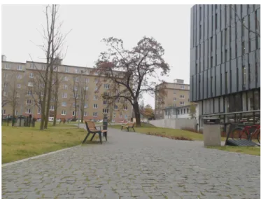
In my experiments, the Otsu’s global threshold method has shown good results in sky detection even without usage of the described modification. In rural areas with forest cover the bright sky was accurately determined even in images where it occupied only approximately 0.33% of potential sky area (at the time upper 60% of an image).
Urban environment was a greater challenge for the algorithm. Some light colored as well as glass covered buildings were occasionally classified as sky in addition to actual sky area. In my opinion, despite the fact that results aren’t entirely accurate, such behavior may be rather beneficial. Light colored buildings would have been likely 19
Chapter 2 Illuminant invariant images
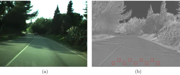
(a) (b)
Figure 8 (a)An example of the image with road. (b)An example of the shadow free image.
deleted with outliers in succeeding algorithms. Therefore the stage at which the building is deleted makes a little difference for outlier detectors with variable threshold, but can be crucial for algorithms based on fixed parameters. Glass buildings can be dangerous for entropy minimization algorithms, as these aren’t Lambertian surfaces and they mostly reflect non desirable sky. If glass buildings are detected and deleted on this stage, they won’t create an additional disruption for entropy minimization algorithms. The other problem typical but not exclusive to urban environments appears, when mobile robot is turned towards a tall object nearby, such as building or dense forest. In such composition, image visible by robot can entirely lack sky area. The proposed sky detection algorithm would still classify the most bright part of an image as sky. This issue wasn’t addressed in the thesis, since this situation isn’t very common. Moreover, in some cases it may be beneficial for above mentioned reasons. In worst case scenario, algorithm would classify as sky less than 50% of image pixels, all located in upper half. This way the most critical part of the road can never be wrongly classified as sky and road detection can still be safely performed.
2.6 Road detection on illuminant invariant image
The shadow-free image obtained using the theory of illuminant invariance is grayscale. An example of such image is shown in figure 8(b) next to the original colorful image in figure 8(a). It can be seen in figure 8(b), that thanks to the illuminant invariance the road region has pixels of the similar values in both shadowed and illuminated areas. This is the property on which this type of road detection algorithms is based.
Since the whole road is of the same color it’s expected of its values histogram to be unimodal with low dispersion and skewness [7]. Under the assumption, that the bottom part of the image is always road, it can be used to build the road model. In this thesis I use 9 regions with the size of 21×21 pixels, placed as depicted in figure 8(b). From
these pixels’ valuesℐ𝑟𝑜𝑎𝑑I create a normalized histogramℋ(ℐ𝑟𝑜𝑎𝑑) and use it to classify
the remaining pixels in the image.
Authors of [7] take the normalized histogramℋ(ℐ𝑟𝑜𝑎𝑑) as a probability distribution
p (ℐ(𝑥)|𝑟𝑜𝑎𝑑). For each unclassified pixel valueℐ(𝑥) they determine its probability of
being road and compare it to the fixed threshold 𝜆. Their classification rule looks like