Evolutionary and Swarm Algorithm Optimized Density- Based Clustering and Classification for Data Analytics

(1)

Evolutionary and Swarm

Algorithm Optimized

Density-Based Clustering and

Classification for Data Analytics

Thesis submitted in accordance with the requirements of the

University of Liverpool for the degree of Doctor in Philosophy

BY

Chun Guan

Department of Computer Science

The University of Liverpool

Liverpool, United Kingdom

(2)

Abstract

Clustering is one of the most widely used pattern recognition technologies for data analytics. Density-based clustering is a category of clustering methods which can find arbitrary shaped clusters. A well-known density-based clustering algorithm is Density-Based Spatial Clustering of Applications with Noise (DBSCAN). DBSCAN has three drawbacks: firstly, the parameters for DBSCAN are hard to set; secondly, the number of clusters cannot be controlled by the users; and thirdly, DBSCAN cannot directly be used as a classifier.

With addressing the drawbacks of DBSCAN, a novel framework, Evolutionary and Swarm Algorithm optimised Density-based Clustering and Classification (ESA-DCC), is proposed. Evolutionary and Swarm Algorithm (ESA), has been applied in various different research fields regarding optimisation problems, including data analytics. Numerous categories of ESAs have been proposed, such as, Genetic Algorithms (GAs), Particle Swarm Optimization (PSO), Differential Evaluation (DE) and Artificial Bee Colony (ABC).

In this thesis, ESA is used to search the best parameters of density-based clustering and classification in the ESA-DCC framework to address the first drawback of DBSCAN. As method to offset the second drawback, four types of fitness functions are defined to enable users to set the number of clusters as input. A supervised fitness function is defined to use the DCC as a classifier to address the third drawback. Four ESA-DCC methods, GA-ESA-DCC, PSO-ESA-DCC, DE-ESA-DCC and ABC-ESA-DCC, are developed. The performance of the ESA-DCC methods is compared with K-means and DBSCAN using ten datasets. The experimental results indicate that the proposed ESA-DCC methods can find the optimised parameters in both supervised and unsupervised contexts. The proposed methods are applied in a product recommender system and image segmentation cases.

(3)

Acknowledgments

I would first like to thank my primary supervisor, Dr. Kevin Kam Fung Yuen, for all the guidance, patience and invaluable encouragement to me. I am really fortunate and honoured to be his first PhD student. I would like to thank my second supervisor, Prof. Frans Coenen, for his support for my work, especially when I studied in the University of Liverpool during my second year. I would also like to take this opportunity to thank my examiners, Prof. Steven Guan and Prof. Jenq-Shiou Leu, for their very helpful comments and suggestions to improve my thesis.

I am very grateful to have been a PhD student of University of Liverpool based on Xi’an Jiaotong-Liverpool University. I am thankful to everyone who have helped me during my PhD study, especially for Prof. Yong Yue and the other staff at the department of Computer Science and Software Engineering, and staff at Research and Graduate Studies Office.

This research is partially supported by the PGR Scholarship of Xi’an Jiaotong-Liverpool University and the University of Jiaotong-Liverpool, the National Natural Science Foundation of China (Project Number 61503306) and the Natural Science Foundation of Jiangsu Province (Project Number BK20150377), China.

Last but not least, I would like to thank my family as well as all of my friends for their continuous supports during my life.

(4)

List of Figures

Figure 2.1 Two Datasets with Arbitrary Shaped Clusters ... 19

Figure 2.2: An Example of Clustering by Dendrogram. ... 23

Figure 2.3 The Procedure of DE [Das & Suganthanm, 2011]. ... 32

Figure 2.5 Four Different Clustering Results of the Sample Dataset ... 46

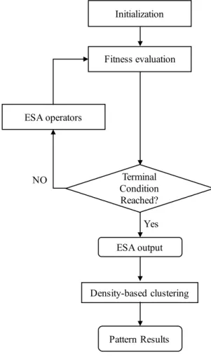
Figure 3.1 The General Procedure of Evolutionary and Swarm Algorithm optimised Density-based Clustering and Classification ... 47

Figure 3.2: Clustering Pattern Results Using ESA-DCC with f_Intor f_Noise as Fitness Function ... 50

Figure 3.3: Results by ESA-DCC with f_K_{as Fitness Function ... 50}

Figures 3.4 Example of Single Point Crossover [Van den Bergh et al., 2004] ... 56

Figures 3.5 Example of Flip Bit Mutation [Van den Bergh et al., 2004] ... 56

Figure 3.6 The Geometrical Interpretation of Two Variants of PSO [Zambrano-Bigiarini et al., 2013]. ... 59

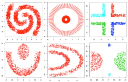
Figure 4.1 Dataset 1-6 ... 65

Figure 4.2 Dataset 7-10 ... 66

Figure 4.3 Convergence Performance of PSO-DCC (SPSO-2011) ... 68

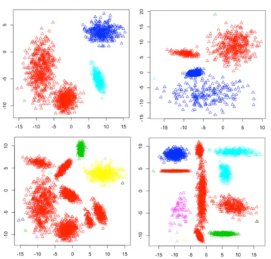
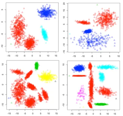
Figure 4.4 Clustering Pattern Results of Datasets 1-6 of Unsupervised PSO-DCC (FNK) ... 70

Figure 4.5 Clustering Pattern Results of Datasets 1-6 of K-means ... 70

Figure 4.6 Clustering Results of Datasets 7-10 Produced by Unsupervised PSO-DCC (FNK) ... 71

Figure 4.7 Clustering Results of Datasets 7-10 Produced by K-means ... 71

Figure 4.8 Pattern Results of Datasets 1-6 Produced by Unsupervised PSO-DCC(SIL) ... 73

Figure 4.9 Pattern Results of Datasets 7-10 Produced by Unsupervised PSO-DCC(SIL) ... 73

(7)

Figure 4.10 Clustering Results of Datasets 1-6 Produced by Unsupervised

PSO-DCC(DB) ... 75

Figure 4.11 Clustering Results of Datasets 7-10 Produced by Unsupervised PSO-DCC (DB) ... 75

Figure 4.12 Prediction Results of Datasets 1-6 Produced by Supervised PSO-DCC .. 77

Figure 4.13 Prediction Results of Datasets 1-6 Produced by SVM ... 77

Figure 4.14 Prediction Results of Datasets 7-10 Produced by Supervised PSO-DCC 78 Figure 4.15 Prediction Results of Datasets 7-10 Produced by SVM ... 78

Figure 4.16 PSO-DCC Results of Dataset 7 with Different Numbers of Clusters ... 79

Figure 4.17 PSO-DCC Results of Dataset 8 with Different Numbers of Clusters ... 80

Figure 4.18 Nomarilized Proceed Time of Four ESA-DCC for 3 Datasets of Different Sizes ... 82

Figure 4.19 The Average Convergence Performance of Four ESA-DCC Methods .... 84

Figure 4.20 Optimized Fitness Values of 4 ESA-DCCs ... 85

Figure 4.21 Rand Index Values of 4 ESA-DCCs (FNK) Clustering Results ... 85

Figure 4.22 Fitness Values of ESA-DCC (FSINK) for Datasets 7-10 and Average .... 86

Figure 4.23 Rand Values of ESA-DCC (FSINK) for Datasets 7-10 and Average ... 87

Figure 4.24. Surface of Fitness Function FNK for Dataset 3 in Range of [0,10] for Minpts and Radius (Left) and in Range of [0,10] for Minpts, [0.4,10] for Radius (Right) ... 88

Figure 4.25 Surface of Fitness Function FNK for Dataset 8 in Range of [0,10] for Minpts and Radius (Left) and in Range of [0,10] for Minpts, [0.7,10] for Radius (Right) ... 89

Figure 5.1 CPR-AHC Framework ... 92

Figure 5.2 Attribute Tree for Laptops ... 98

Figure 5.3 Orginal Images. ... 107

Figure 5.4: Segmentation Results of Kmeans-DBSCAN by Setting K as 50, DBSCAN Parameter Pairs as: (a) (0.40, 2); (b) (0.35, 3); (c) (0.31, 2); (d) (0.33, 3) ... 109

(8)

Figure 5.5: Segmentation Results of Kmeans-DBSCAN by Setting K as 100, DBSCAN Parameter Pairs as: (a) (0.25, 3); (b) (0.35, 5); (c) (0.31, 4); (d) (0.33, 5) ... 109 Figure A1. Interface for Comparison Pairwise Rating of Laptop Attributes ... 114

(9)

List of Tables

Table 2.1 Clustering Validation Indices Used as Fitness Functions ... 43

Table 2.2 Sample Dataset ... 44

Table 2.3 Clustering Results of Sample Dataset ... 45

Table 3.1 Computational Complexities of Proposed Fitness Functions ... 52

Table 4.1 Description of Datasets ... 65

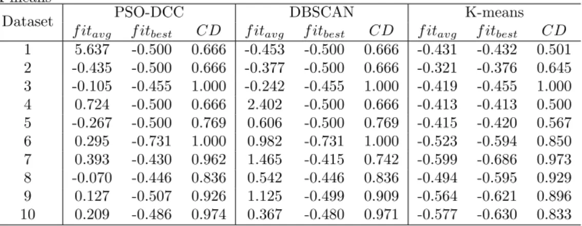
Table 4.2 Unsupervised PODCC with FNK versus DBSCAN and K-means ... 69

Table 4.3 Unsupervised PODCC with Silhouette Index versus DBSCAN and K-means ... 72

Table 4.4 Unsupervised PODCC with Davies Bouldin Index versus DBSCAN and K-means ... 74

Table 4.5 Supervised PODCC with Czekanowski-Dice Index versus SVM ... 76

Table 4.6 Parameter Settings for Four ESA-DCC methods ... 81

Table 4.7 Coverage of Four Proposed Methods ... 83

Table 4.8 Unsupervised ESA-DBCs with FNK ... 84

Table 4.9 Unsupervised ESA-DBC with FSINK ... 86

Table 4.10 Unsupervised ESA-DBC with FDBNK ... 87

Table 4.11 Unsupervised ESA-DBC with FCD ... 88

Table 5.1: Measurement Scale Schema for CPR ... 94

Table 5.2: Schema of Leaf Attributes of Laptops ... 99

Table 5.3: Comparison Matrices for Laptop 1st Level Attributes of User A ... 100

Table 5.4: Comparison Matrices of User A for Laptop Sub-attributes ... 101

Table 5.5: Comparison Matrices of User A for Nominal Attribute of L2, L6, and L7 . 101 Table 5.6: Laptop Product Values for User A ... 103

Table 5.7. The Top-10 Laptops for User A ... 104

Table 5.8. Clustering Results of Laptops. ... 104

(10)

Table A1: Computational Details of AI for Nominal Attribute of L7 ... 115

Table A2: Raw Matrix D of 27 Laptops ... 116 Table A3: Normalized Data Matrix D’ of 27 Laptops for User A ... 117

(11)

List of Algorithms

Algorithm 2.1: K-means ... 21

Algorithm 2.2: DBSCAN ... 24

Algorithm 2.3: A Simple GA ... 30

Algorithm 2.4: General PSO Procedures ... 32

Algorithm 2.5: ABC Algorithm ... 33

Algorithm 3.1. GA-DCC... 53

Algorithm 3.2: Fitness Proportionate Selection ... 55

Algorithm 3.4: DE-DCC. ... 60

Algorithm 3.5 ABC-DCC. ... 61

Algorithm 5.1: Top-N List ... 96

(12)

Chapter 1 Introduction

Data analytic has attracted significant attention in the information industry and society, due to the huge amounts of data and the increasing need for turning such data into useful information and knowledge [Han, Pei, and Kamber, 2011]. Clustering Analysis is a widely used pattern recognition technology in the field of data analytic. Clustering methods can be categorized into Partional-based methods, Hierarchical-based methods, Density-based methods, Grid-based methods, Model-based methods and so on. Density-based clustering was proposed to deal with spatial datasets such as satellite images, facial images and medical images [Ester et al., 1996]. The best-known density-based clustering algorithm is the Density-Based Spatial Clustering of Applications with Noise (DBSCAN) [Ester et al., 1996]. DBSCAN uses two parameters, the radius of hyper-spheres (!) and the minimum number of points in each hyper-sphere (minpts). The main advantage of DBSCAN is its ability to find arbitrary shaped clusters through detecting the high-density hyper-spheres and merging the close hyper-spheres into clusters. In contrast, the centroid-based clustering method cannot be used to find arbitrary shaped clusters in spatial datasets. Conversely, Hierarchical-based clustering can be applied to spatial datasets, although, the clustering results are sensitive to noise. However, DBSCAN has some limitations. Firstly, the parameters for DBSCAN are hard to set, the two parameters, radius (!) and the minimum number of points (minpts), are often set by manual testing. Although, some parameter-tuning methods require one pre-defined parameter to calculate another parameter, for instance, the k-distance plot method requires a pre-defined minpts to find the corresponding suitable !. Secondly, the known number of clusters cannot be used in the clustering process. For some clustering methods, the number of clusters is known beforehand which can be used to aid the clustering process. For example, the number of clusters is the only input parameter for K-means. Similarly, the known number of clusters can be used to decide

(13)

how to cut the tree structure produced by hierarchical clustering method. However, the number of clusters cannot be controlled by the users in DBSCAN. Thirdly, DBSCAN cannot be directly applied for classification purposes.

The central motivation for this research is the intuition that Evolutionary and Swarm Algorithms (ESAs) [Fogel, 2006] could be used as a parameter-tuning tool for DBSCAN. Evolutionary Computing (EC) and Swarm Intelligence (SI) can generally be described as Evolutionary and Swarm Algorithms (ESAs). Numerous categories of ESAs have been proposed, these include: Genetic Algorithms (GAs) [Golberg,1989], Particle Swarm Optimization (PSO) [Kennedy, 1995], Differential Evaluation (DE) [Storn & Price, 1997], Artificial Bee Colony (ABC) [Karaboga, 2005], etc. GA and DE are two typical types of evolutionary algorithms. PSO and ABC are two examples of ESA methods. The development of ESAs was inspired by the idea of natural selection and observations of animal behaviour. For example, GA is inspired by the mechanism of natural selection; the operators in GA algorithms and evolutionary strategies are the motivators behind DE; the social conduct of groups of animals, such as flocks of birds, schools of fish and herds of mammals, stimulated the development of PSO; and similarly, ABC is inspired by the behaviour of bees when searching for food sources The main advantage of ESA is the highly robust search performance of such algorithms. In this thesis, ESA methods are applied as parameter tuning tools to offset the first drawback of DBSCAN. ESAs have been applied as the optimisation methods for various clustering methods. Various ESA optimal clustering methods have been reviewed in Section 2 of this work.

Based on the above observations, a novel framework, Evolutionary and Swarm Algorithms Optimised Density-based Clustering and Classification (ESA-DCC), is proposed directed at optimising the performance of density-based clustering by finding the best parameter settings through a search of the entire parameter space using ESAs. In this framework, two types of fitness functions are designed on the basis of the current

(14)

clustering validation indices; and penalty functions are designed to minimise the number of noises and to control the number of clusters. In this thesis, four types of ESAs (GA, PSO, DE and ABC) are adopted in the ESA-DCC framework. The Four ESA-DCC methods are evaluated by both experimental cases and real-world problems. The main contributions of this work are the proposal of the structure of applying ESA to tune the parameters for density-based clustering methods and the proposal of fitness functions for the ESA optimised density-based clustering methods framework. With the structure and these fitness functions, any ESA could be applied to optimise a density-based clustering method. The ESA-DCC framework could be extended by adopting original and revised ESAs as well as density-based clustering methods. The proposed fitness functions are reasonable combinations of available components: the clustering index, the penalty function to minimize the number of noises and the function to control the number of clusters. The various functions of the different choices of components and clustering indices are be flexibly applied to clustering problems on a case-by-case basis.

The proposed ESA-DCC methods can be applied to find the arbitrary shaped clusters in spatial datasets. For the datasets which are not well understood, the proposed ESA-DCC method can be applied to search for possible clustering patterns by testing with different number of clusters. For the datasets with a known number of clusters, the proposed ESA-DCC method can find a set of parameters to produce the optimum clustering results.

Some limitations of the proposed ESA-DCC framework are evident. Firstly, the computational complexity of the proposed ESA optimised DBSCAN framework (ESA-DCC) is limited by the complexity of the DBSCAN method. The computational complexity of a standard DBSCAN method is as high as Ο #log # . Since ESA-DCC adopts the standard DBSCAN, and the DBSCAN runs multiple times to reach the optimal solution in ESA-DCC, the complexity of ESA-DCC is higher than that of

(15)

DBSCAN. Secondly, the clustering indices applied in the fitness functions may not be suitable for non-centroid clusters since the indices were proposed for measuring the goodness of centroid-based clusters. A proposal for a clustering index for density-based clustering results will be explored in the future work of this research. Thirdly, the weights for the components of a fitness function need to be further investigated.

Six academic papers presenting the reseach work in this thesis have been accomplished and listed below.

(1) Guan, C., & Yuen, K. K. F., Towards a hybrid approach of primitive cognitive network process and agglomerative hierarchical clustering for music recommendation. In Heterogeneous Networking for Quality, Reliability, Security and Robustness (QSHINE), 2015 11th International Conference on (pp. 206-209), IEEE, 2015.

(2) Guan, C., Yuen, K. K. F., & Coenen, F., Towards an intuitionistic fuzzy agglomerative hierarchical clustering algorithm for music recommendation in folksonomy. In Systems, Man, and Cybernetics (SMC), 2015 IEEE International Conference on (pp. 2039-2042), IEEE, 2015

(3) Guan, C., Yuen, K. K. F., & Chen, Q. (2017, June). Towards a Hybrid Approach of K-Means and Density-Based Spatial Clustering of Applications with Noise for Image Segmentation. In Internet of Things (iThings) and IEEE Green Computing and Communications (GreenCom) and IEEE Cyber, Physical and Social Computing (CPSCom) and IEEE Smart Data (SmartData), 2017 IEEE International Conference on (pp. 396-399). IEEE.

(4) Guan, C., & Yuen, K. K. F., The Cognitive Pairwise Rating Agglomerative Hierarchical Clustering for A Recommender System: An Application of Laptop Recommendation. Submitted to journal.

(16)

(5) Guan, C., Yuen, K. K. F., & Coenen, F., Particle Swarm Optimized Density-Based Clustering and Classification: Supervised and Unsupervised Learning Approaches. Submitted to journal.

(6) Guan, C., Yuen, K. K. F., & Yue, Y., Towards A Personalized Item Recommendation Approach in Social Tagging Systems Using Intuitionistic Fuzzy DBSCAN. Submitted to conference.

This thesis consists of 6 chapters and organized as below.

l Chapter 1 is the introduction, describing the context of the thesis and briefly

introducing the background and motivation of the proposed framework.

l Chapter 2 is the literature review of the research area. This chapter reviews the

details of clustering analysis and Evolutionary and Swarm Algorithms (ESAs). Three major types of clustering technologies and the corresponding representative algorithms are examined. Four mainstream ESAs, GA, PSO, DE and ABC, which will be used along this work are studied in this chapter. A number of representative hybrid methods of Clustering and ESA are also reviewed and summarized. The motivation of this work is proposed in this chapter by comparing and discussing the current methods.

l Chapter 3 proposes the framework of ESA optimised density-based clustering

methods. The four ESA methods that are reviewed in Chapter 2 are applied in the framework. The design and implementation of the proposed ESA optimised density-based clustering methods are described in detail.

l Chapter 4 presents the experimental design and results for the proposed methods.

The propositioned methods are evaluated by 10 datasets and compared with K-means and DBSCAN. By analyzing the experimental results, the strengths and limitations of the methods are highlighted.

(17)

l Chapter 5 presents two types of applications for the proposed methods for a

number of real world problems. The suggested methods are demonstrated for the applications of recommender systems and image segmentation. Furthermore, the proposed method integrated with Cognitive Pairwise Rating (CPR), an ideal alternative of AHP, is applied to the personalized recommender system.

(18)

Chapter 2 Literature Review

The literature review covers three main sections: a review of clustering algorithms, an study of Evolutionary and Swarm Algorithms (ESAs), and a appraisal of current hybrid methods of clustering and ESAs.

2.1 Clustering Analysis

Clustering is an example of unsupervised learning in the machine learning field. The process of clustering can be described as grouping a set of objects into clusters with respect to the dissimilarities between them. The data objects in one cluster are similar to each other and dissimilarfrom the objects in other clusters. Cluster analysis has many functions in numerous data analytic applications, such as market analysis, pattern recognition and image processing. Clustering methods can generally be categorized into several classifications, such as Partional-based methods, Hierarchical-based methods, Density-based methods, Model-based methods and etc. The three mainstream categories of clustering methods are reviewed in Sections 2.1.1-2.1.3. Some of the basic conceptions and terminologies for clustering methods are reviewed according to the descriptions in [Han et al., 2011].

• Data Matrix

A dataset to be clustered can be represented as a data matrix. Each row of the matrix represents an object with its attributes. The structure of a n-by-p data matrix which contains #×( objects is shown in the form below.

2 6 6 6 6 4 x11 ... x1f ... x1p ... ... ... ... ... xi1 ... xif ... xip ... ... ... ... ... xn1 ... xnf ... xnp 3 7 7 7 7 5 (2.1)

(19)

• Different Types of Attributes

The attributes of each object vary depending on the meaning of the attribute value. The typical attribute types for measuring an variable are introduced as below.

Interval-Scaled Attributes are continuous measurements of a roughly linear scale, such as weight, height, weather temperature, latitude and longitude.

Binary Attributes have only two possible values, 0 or 1. The values indicate that the variable is absent (represented by 0) or present (represented by 1). It can be regarded as an “Yes or No” answer to a question for each individual. For example, for the attribute “marital status”, 0 means single and 1 means married. The meaning of 0 or 1 can also be pre-defined, such as for the attribute “gender”, 0 can be defined as female whilst 1 would be male and vice versa.

Categorical Attributes can be regarded as the generalizations of binary variables which can take on more than two states, such as color, brand, shape and so on. Ordinal Attributes are a number of values which can be ordered in a meaningful sequence. One of the most famous example of ordinal variables is the three kinds of medals given out for a sporting competition: gold, silver and bronze.

• Dissimilarity Matrix

The proximities for all pairs of n objects can be represented by an n-by-n table shown as below, where d(i, j) is the measured by the dissimilarity between objects i and j.

2 6 6 6 6 6 4 0 d(2,1) 0 d(3,1) d(3,2) 0 .. . ... ... d(n,1) d(n,2) · · · 0 3 7 7 7 7 7 5 (2.2)

(20)

As a wildly used distance measure, Euclidean distance is suitable for measuring the dissimilarities between objects with multiple attributes. The computation of Euclidean distance is defined as below.

Note that this type of distance measure can only be applied to the interval-scaled attributes. The other types of attributes can be transferred into interval-scaled attributes in a preprocessing stage, before using the Euclidean Distance. In this research, the data preprocessing steps are mainly conducted by PCNP [Yuen, 2009; 2012; 2014(1); 2014(2)] to deal with the difference types of attributes. The preprocessing steps are introduced in Section 5.1.2 with real-world cases.

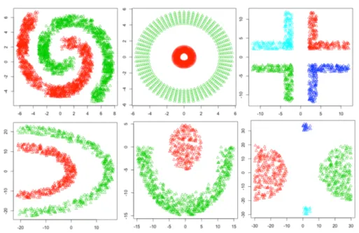
Arbitrary Shaped Clusters

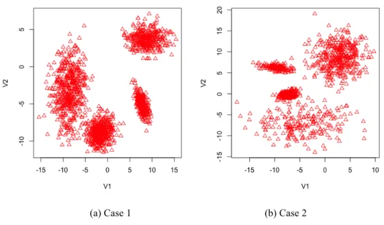
Some datasets include arbitrary shaped clusters, which means that the clusters are not centroid based, for instance, a dataset transferred from a digital facial image. Figure 2.1 presents two examples of a dataset consisting of arbitrary shaped clusters. Since most of the partitional based clustering methods are centroid based, such as means and K-centroid, the other types of clustering methods are applied to process this particular kind of dataset, such as hierarchical and density-based clustering methods.

Figure 2.1 Two Datasets with Arbitrary Shaped Clusters

(21)

• Noisy Data \ Noise

In this work, the term noise (noisy data) refers to an object which is not assigned to any cluster. The detection of noise is a topic in clustering analysis. Some clustering methods, such as K-means, do not directly deal with noise, as a consequence, the noise in the ground truth partitions may lead to poor clustering results in the pattern of results when using such a method.

2.1.1 Partitioning Clustering

A partitioning clustering algorithm can organize a data set D of n objects into k clusters, where k ≤ n. The clusters are formed to optimise an objective partitioning criterion, for example, to minimize a dissimilarity value based on distance to ensure the objects within a cluster are similar, whilst the objects of different clusters are dissimilar. The most widely used and classical partitioning clustering method is K-means.

K-means

The K-means algorithm [MacQueen, 1967; Jain, 2009] takes a parameter, k, as input, and assigns n objects into k clusters resulting in the similarity of the objects within each cluster being high but the similarity between the objects in different clusters being low. Typically, the aim of the K-means process is to minimize the total mean-square quantization error (MSE) until the criterion function converges. The function to compute MSE is defined as below.

where E is the sum of the square error for all objects in the data set; p is the point in space representing a given object; and mi is the mean of cluster Ci (both p and mi are

multi-dimensional). The mean value of the objects in a cluster is regarded as the

E = k X i=1 X p2Ci |p mi| (2.4)

(22)

cluster’s centroid. The criterion is the sum of the squared distance from the object to its cluster center. The pseudo code of classical K-means [MacQueen, 1967] is provided in Algorithm 2.1 as below.

Algorithm 2.1: K-means

Input: k: the number of clusters, D: a data set containing n objects.

Output: A set of k clusters.

1. Arbitrarily choose k objects from D as the initial cluster centers;

2. Assign each object to the cluster to which the object is the most similar, based on the mean value of the objects in the cluster;

3. Update the cluster means, i.e., calculate the mean value of the objects for each cluster;

4. Repeat steps 2-3 until no change.

2.1.2 Hierarchical Clustering

The hierarchical clustering method works by building a tree structure of the objects in a dataset. There are two major methods for Hierarchical clustering methods:agglomerative and divisive. For agglomerative methods, tree structures are built from the bottom up, and for divisive ones, the trees are built from the top down.

• Agglomerative hierarchical clustering starts by regarding each object as an atomic cluster and then merges these atomic clusters into larger clusters. This step is repeated until all of the objects are in a single cluster or until a certain termination condition is satisfied. The majority of hierarchical clustering methods belong to this category, they differ only in the computational style of the inter-cluster similarity. The details of typical AHC are introduced in this section.

• Divisive hierarchical clustering does the reverse of agglomerative hierarchical clustering by starting with putting all objects in one cluster, and then dividing the

(23)

cluster into increasingly smaller clusters, until each cluster only contains one object, or until a certain termination conditions is satisfied. There are less hierarchical clustering algorithms which follow this strategy.

Agglomerative Hierarchical Clustering

The original Agglomerative Hierarchical Clustering (AHC) [Ward, 1963] was proposed more than half a century ago. In AHC, the pairs of closest clusters are iteratively merged into larger clusters until all of the objects are in a single cluster or a termination condition is satisfied [Han et al, 2011]. The three main steps of hierarchical clustering methods are summarized below with reference to [Murtagh, 1983].

i. Initialization: each object is initialized as an atomic cluster. The dissimilarities between atomic clusters can be computed in different ways, this was introduced in Section 2.1.1.

ii. Merging: the two closest clusters, Ci and Cj,are combined to form a larger cluster.

The four mainstream measurements for choosing the closest pair of clusters for inter-cluster similarity are shown below, where p is an object, mi is the centroid of

clusters Ci, and ni is the number of objects in cluster Ci • Minimun\Single-linkage:

• Maximun\Complete-linkage:

• Centroid-linkage:

• Average-linkage

This step should be repeated until all objects are in one cluster.

dmin(Ci, Cj) = min p₂Ci,p02Cj| p p0| (2.5) dmax(Ci, Cj) = max p₂Ci,p02Cj| p p0_| (2.6) dmean(Ci, Cj) =|mi mj| (2.7) davg(Ci, Cj) = 1 ninj X p2Ci X p0₂_C_j |p p0_| (2.8)

(24)

iii. Clusters generation: a dendrogram is used to illustrate the arrangement of the merged clusters. The objects are divided into different clustering patterns by cutting the branches at an appropriate height, which is represented by the dissimilarity between clusters. For example, the dendrogram shown in Figure 2.2 can be cut by Line A and then three clusters are generated. Similarly, the dataset can be divided into five clusters if the dendrogram is cut by Line B.

Figure 2.2: An Example of Clustering by Dendrogram.

2.1.3 Density-based Clustering

Density-based clustering methods can be used to discover clusters with arbitrary shape. The dense regions of objects in the data space are recognized as clusters, and the regions of low density are marked as noisy points (or noises). Thus, the DBSCAN grows clusters according to a density-based connectivity analysis. A number of hybrid and enhanced density-based clustering methods have been developed, for example: l-DBSCAN [Viswanath & Pinkesh, 2006], ST-l-DBSCAN [Birant & Kut, 2007], Rough-DBSCAN [Viswanath & Babu, 2009], P-Rough-DBSCAN [Kisilevich, Mansmann & Keim, 2010], MR-DBSCAN [He, Tan, Luo, Mao, Ma, Feng & Fan, 2011], PDS-DBSCAN [Patwary, Palsetia, Agrawal, Liao, Manne & Choudhary, 2012], Revised DBSCAN

(25)

[Tran, Drab & Daszykowski, 2013] and G-DBSCAN [Andrade, Ramos, Madeira, Sachetto, Ferreira & Rocha, 2013]. The details of DBSCAN are reviewed in this section.

DBSCAN

Density-Based Spatial Clustering of Applications with Noise (DBSCAN) was originally proposed in 1996 [Ester et al., 1996]. DBSCAN can easily find the arbitrary shape of clusters by detecting the high-density hyper-spheres and merging the close hyper-spheres into clusters. As already noted, DBSCAN uses two critical parameters, the radius of hyper-spheres (ϵ) and the minimum number of points in each hyper-sphere (Minpts), the clustering results of DBSCAN are sensitive to the values of these two parameters. The pseudo code for the DBSCAN algorithm is given in Algorithm 2.2.

Algorithm 2.2: DBSCAN

Input: Dataset S, Radius of each hyper-sphere ϵ the minimum number of points in the hyper-sphere, MinPts.

Output: Pattern Result, (PR). 1. Initialize cid = 0;

2. For each individual in dataset, i.e. s∈S,

If s is not marked as “seen”, then Mark s as “seen” and find Nϵ(s; S), If card(Nϵ(s; S)) < MinPts, then (PR)_sid₍_s_{) =0;}

else cid = cid + 1, (PR)_sid₍_s_{) =}cid;

For s’∈Nϵ(s; S) and s’ is not marked as “seen”, Mark s’ as “seen”;

Find Nϵ(s’; S);

If card(Nϵ(s; S))≥MinPts, then (PR)_sid₍_s’_{) =}cid;

else continue next point 3. Return (PR).

The clustering Pattern Result (PR) is a list [c1,c2,...,cn] where each element ci is a cluster

(26)

dataset S, and the indexes indicate individual record numbers for each record s in S. A mark seen is used to distinguish between the records which have been processed and those which still need to be processed. ,-(s; S) is a function that returns the subset of records in S, that are present in a particular cluster (hyper-sphere) of radius ., that s in

S belongs to card(,-(s; S)) returns the cardinality of the set ,-(s; S); whilst sid(s) returns the index in PR of s in S. The drawbacks of DBSCAN are discussed in Section 2.4 as a part of the research limitations.

2.2 Evolutional and Swarm Algorithms

2.2.1 Introduction

Evolutionary and Swarm Algorithms (ESAs) are some Computational Intelligence (CI) methods were inspired by the evolution of species and the behaviors of animals in swarms. This work covers four typical and widely used ESAs, Particle Swarm Optimization (PSO) [Kennedy, 1995], Artificial Bee Colony (ABC) [Karaboga, 2005], Genetic Algorithms (GAs) [Golberg,1989] and Differential Evaluation (DE) [Storn & Price, 1997]. The common use of each ESA is to be applied in an optimisation problem which find a set of parameter values that minimize or maximize a function in a pre-defined search space.

GA is the mainstream algorithm of evolutionary algorithms. The initial conception that the evolution could be applied in the process of optimisation has been proposed since the 1960s [Holland, 1962]. The theory of GA has been further developed by the team led by John Holland in the following decades [Holland, 1975; Holland, Holyoak, Nisbett, & Thagard, 1986]. The applications of GAs were further investigated during the 1980s [Goldberg, 1989; Grefenstette, 1985, 1987; Goldberg & Holland, 1988]. In this work, the canonical genetic algorithm is applied to develop the initial approaches and compare with other methods.

(27)

PSO was inspired by the swarming behavior that was displayed by a flock of birds, a school of fish, or even human social behavior being influenced by other individuals [Kennedy, 1995]. The developments, applications and resources of PSO before the year 2001 were summarised in [Shi, 2011]. The PSO methods developed for solving constrained optimisation problems were summarized in [Parsopoulos & Vrahatis, 2002]. Some PSO variant algorithms were proposed since the initial PSO was suggested. A standard of PSO was defined in 2007 [Bratton & Kennedy, 2007] to compare and summarize three types of PSO including original PSO, Constricted GBest and Constricted LBest. The variants were implemented and summarized in a famous R package hydroPSO [Zambrano-Bigiarini & Rojas, 2013; Zambrano-Bigiarini, Clerc & Rojas, 2013]. The different PSO algorithms presented in hydroPSO are Standard PSO 2011 (spso2011) [Clerc, 2012], Standard PSO 2007 (spso2007) [Clerc, 2012], Fully Informed Particle Swarm (fips) [Mendes, 2004], Weighted Fully Informed Particle Swarm (wfips) [Mendes, 2004], Improved PSO (IPSO) [Zhao, 2006] and Canonical PSO [Clerc, 2009]. In this work, Canonical PSO and SPSO 2011 are applied in the proposed framework. An application of this package including a detailed illustration was presented in 2013 [Zambrano-Bigiarini & Rojas, 2013]. The two reviews of PSO presented in [Banks, Vincent & Anyakoha, 2007, 2008] covers the development, hybridization and application of PSO. [García-Gonzalo & Fernández-Martínez, 2012] is a recent summary of PSO methods in 2012.

As an evolution strategy, the DE algorithm was introduced by Storn and Price in the 1990s [Storn & Price, 1997; 1995]. DE is particularly compatible to find the global optimum of a real-valued function of real-valued parameters and does not require that the function to be either continuous or differentiable. In the roughly fifteen years since its invention, DE has been successfully applied in a wide variety of fields, from computational physics to operations research [Price, Storn & Lampine, 2006]. A recent review of DE was presented in [Das, Mullick & Suganthan, 2016].

(28)

ABC were firstly defined in 2005 by Karaboga [Karaboga, 2005]. The computational processes and application areas of ABC were further extended in 2007 [Karaboga & Basturk, 2007]. The performance of ABC was compared to other EC methods such as DE, PSO and GA in [Karaboga & Basturk, 2008]. The optimisation results of the five functions demostrate that ABC algorithm performed better than the aforementioned algorithms in [Karaboga & Basturk, 2008]. Due to several insufficiencies in classical ABC, some improved ABC algorithms have been proposed. To improve the exploitation of classical ABC, the Gbest-guided artificial bee colony (GABC) was developed by incorporating the information of the global best (gbest) solution into the solution search equation in 2010 [Zhu & Kwong, 2010]. A modified ABC was developed for real parameter optimisation [Akay & Karaboga, 2012]. The development and application of ABC were reviewed in [Karaboga & Akay, 2009; Karaboga, Gorkemli, Ozturk & Karaboga, 2014].

Some comparative research has been studied to discuss the superiority of one EC method over the others. For example, [Eberhart & Shi, 1998] is a comparison between GA and PSO in 1998, similarly, [Civicioglu & Besdok, 2013] reviewed and compared PSO, DE and ABC in 2011. More reviews are mentioned in Section 2.3.1 and are conducted with respect to certain applications of ESA methods, such as optimising the performance of clustering analysis.

2.2.2 Basic Concepts

The general procedures of ESAs could be summarized as a group of candidate solutions moving in a pre-defined space in particular patterns and finally the best solution among all the candidate solutions is produced as the optimised solution. The steps of all the ESAs consist of two phases: representing the solutions as a swarm or genetics and searching for the best member of a swarm or the best chromosome of a gene pool in a search space. The common or similar terminologies applied in ESAs are introduced in

(29)

this section, they include encoding, search space, fitness function, stopping criteria, etc. The details of the common terminologies are explained below.

• Solution Representation

There are three major ways of representing candidate solutions which are applied in ESAs: binary representation, integer representation and real-valued representation. All the representation forms can be applied in GA and the real-valued representation can be applied to PSO, DE and ABC.

In GA, each candidate solution can be encoded as a “chromosome” consisting of a number of “genes”, in comparison, for the binary representation, each solution is denoted as a bit-string. The integer representation is applied in GA, whilst the candidate solutions include ordinal parameters or cardinal attributes. Each solution is represented by a vector of integers which signify a particular meaning. This occurs when the values to be represent as genes come from a continuous rather than a discrete distribution. For example, if they represent physical quantities, such as the length, width, height, or weight of a component of a design, that can be specified within a tolerance smaller than integer values.

In PSO, each candidate solution is represented as a particle; and all the particles form the swarm. In DE, each agent represents one candidate solution. Similarly, food sources are the candidate solutions in ABC.

• Objective Function and Fitness Function

For an ESA, the problem to be solved is represented as an objective function. A fitness function is designed as a particular type of the objective function, to evaluate how well the candidate solutions solve the problem.

For example, GA often requires a fitness function that assigns a score (fitness) to each chromosome in the current population. The fitness of a chromosome depends on how

(30)

well that chromosome solves the problem at hand. Similarly, PSO requires a fitness for each particle; ABC needs a fitness for each food source; and DE requires a fitness for each agent.

• Search Space

All the candidate solutions are randomly generated in the search space, which means a pre-defined range of each parameter of solutions. The dimension of the search space is the number of parameters in each candidate solution and the minimum and maximum values for each dimension should be pre-defined to determine the whole scope of the search space.

• Stopping Criteria or Convergence Tolerance

According to the summarization presented in [Eiben & James, 2003], the four major types of stopping criteria shown below can be applied in all the ESAs.

1. The maximum allowed CPU time elapses.

2. The total number of fitness evaluations reaches a given limit.

3. The fitness improvement remains under a threshold value for a given period of time, which means the algorithm’s solution has been converged.

4. The population diversity drops under a given threshold.

2.2.3 Genetic Algorithm

Genetic algorithms (GAs) were created by John Holland in the 1960s and were further developed by his research group at the University of Michigan in the following decades. During the past half century, researchers have studied and developed the concept of GAs and broke the boundaries between GAs, evolution strategies, evolutionary programming, and other evolutionary approaches. Nowadays, the term “Genetic Algorithm” can be used to describe a number of various algorithms which could vary

(31)

from the original GA method. In this work, the GA method mentioned mainly follows the Genetic Algorithms defined by [Mitchell, 1989] and [Eiben & James, 2003].

Algorithm 2.3: A Simple GA

1 Start with a randomly generated population of n chromosomes. 2 Calculate the fitness of each chromosomein the population. 3 Repeat the following steps until n offspring have been created:

3.1 Select a pair of parent chromosomes from the current population.

3.2 With the crossover probability, cross over the pair at a randomly chosen point to generate two offspring. If no crossover takes place, copy the parents as the two offspring.

3.3 Mutate the two offspring at each locus with the mutation probability and place the resulting chromosomes in the new population.

4 Replace the current population with the new population. 5 Loop step 2-4 until the stop criteria is reached.

6 Output the best population with highest fitness.

A simple procedure of GA is presented in Algorithm 2.3 with respect to the context of [Mitchell, 1998]. Each iteration (Steps 2-4 in Algorithm 2.3) of this process is called a generation and a GA is typically iterated for hundreds of generations. The entire set of generations is called a run, at the end of the run, there are often one or more highly fit chromosomes in the population. As the algorithm demonstrates, the simplest form of a genetic algorithm involves three types of operators: selection, crossover, and mutation.

• Selection

Selection is the process to find the individuals with a higher fitness to produce the next generation. Typically, parent selection technologies are probabilistic in GAs. The high-quality individuals have high probabilities to be selected as parent, whilst the low-quality individuals have a chance to be selected but the chance is very small, such that the search cannot be too greedy to get stuck in a local best solution. For example, some

(32)

widely used selections are roulette-wheel selection (also named as fitness proportionate selection), tournament selection, reward-based selection, and etc. In this work, the roulette-wheel selection is applied in the proposed GA-based clustering method described in Section 3.2.

• Crossover

Crossover (or sometimes referred to as recombination) is an operator which merges two individuals (which refers to the parents selected by the selection operator) into offspring individuals. The principle aim of the crossover is to mate two individuals with different but desirable features to produce an offspring that combines both of those features. This principle is inspired by produce species that give higher yields or have other desirable features in the area of plant and livestock breeders.

In GAs, the offspring (next generation) are produced by a random recombination which is named as a crossover. A crossover is a stochastic operator, which means that the choices of what parts of each parent are combined are randomly decided with respect to a pre-defined crossover rate. A crossover is also applied probabilistically, which means the parents have a small predefined chance not to be performed crossover. The offspring of a pair of parents are the same as themselves if no crossover is performed. Various crossover methods are proposed with respect to the different genotypes (decoding style) of chromosomes. For example, the bit-string chromosomes, single-point, two-single-point, and uniform crossover. In this work, the single-point crossover is applied in the proposed GA-based clustering method described in Section 3.2.

• Mutation

Mutation is a unary variation operator in GAs. A mutation operator is stochastically preformed to one bit (genotype) of the offspring generated by the stage of crossover, a slightly changed mutant can be generated by the mutation operator.

(33)

2.2.4 Particle Swarm Optimization

PSO is a population based stochastic optimisation technique to find the best fitting solution. PSO has a number of advantages, such as flexibility, easy computational implementation, low computational requirements, low number of parameters, and efficiency [Eberhart and Shi, 1998; Shi and Eberhart, 1999; Eberhart and Shi, 2001; Poli et al., 2007]. Numerous variants of the original PSO algorithm have been proposed to further improve the performance of PSO (see Section 2.2.1 for details). The general procedures of PSO are presented as Algorithm 2.4. Two versions, the canonical PSO and the Standard PSO proposed in 2011 (SPSO-2011), are reviewed and applied in this work (see Section 3.3 for detail).

Algorithm 2.4: General PSO Procedures

1 Initialize the velocity and position of each particle.

2 Loop until the maximum iterations or minimum error criteria is reached. 2.1 Calculate fitness value

2.2 If the fitness value is better than the best fitness value (pBest) in history, then set current value as the new pBest

2.3 Choose the particle with the best fitness value of all the particles as the gBest

2.4 Calculate and update the velocity and position of each particle. 3 Output the best particles.

2.2.5 Differential Evolution

Differential Evolution (DE) was originally developed in 1995 by Storn and Price. The main procedure of DE is shown in Figure 2.3. Similar to that of GA, DE also has three operators, mutation, recombination (also can be named as crossover), and selection, but in a different order.

(34)

The advantages of DE have been summarized in [Storn et al. 1997] and are as follows:

• ability to handle non-differentiable, nonlinear and multimodal cost functions.

• parallelizability to cope with computation intensive cost functions.

• ease of use, since few control variables are required to steer the minimization.

• good convergence propertie.

The details about the DE algorithm are presented within the proposed DE-DCC method in Section 3.4.

2.2.6 Artificial Bee Colony Algorithm

ABC is proposed to model the specific intelligent behaviors of honey bee swarms and applies to solving combinatorial type problems. In the ABC algorithm, the candidate solutions of object functions are the food sources which can be selected or discarded by bees. The colony of artificial bees contains three groups of bees: employed bees, onlookers and scouts. A bee waiting in the dance area to make a decision to choose a food source, is called an onlooker, whereas, a bee going to the food source visited by itself previously is termed an employed bee. The bee that searches around randomly is called scout. In the ABC algorithm, half of the bees are employed artificial bees and the other half are the onlookers. One employee bee is in charge of one food source. In other words, the number of employed bees is equal to the number of food sources. The employed bee whose food source is exhausted by the employed and onlooker bees becomes a scout. The main steps of ABC algorithm (which revises and improves the presentation of the paper [Karaboga, 2005]) are given in Algorithm 2.5.

Algorithm 2.5: ABC Algorithm

1 Send the scouts onto the initial food sources 2 Repeat from 2 until requirements are met.

2.1 Send the employed bees onto the food sources and determine their nectar amounts

2.2 Calculate the probability value of the sources with which they are preferred by the onlooker bees

(35)

2.3 Send the onlooker bees onto the food sources and determine their nectar amounts

2.4 Stop the exploitation process of the sources exhausted by the bees 2.5 Send the scouts into the search area for discovering new food sources,

randomly

2.6 Memorize the best food source found so far 3 Output Best food source.

2.3 Hybrid Approaches of ESAs and Clustering

2.3.1 General Review

ESA algorithms have been widely applied in data mining fields such as clustering analysis. The fact that they are easy to be trapped in local best result is one of the main problems existing in classical clustering method. The main advantage of ESA is the stochastic optimisation, which can overcome the drawback of the search strategy in the classical clustering method. To improve the efficiency and accuracy of the classical clustering analysis algorithms, the clustering problems could be represented as functions to be optimised by ESA technologies. Some reviews have been made in the past two decades to summarize the various ESA optimised clustering algorithms. A more detailed review of GA-based clustering methods was accomplished by presenting the framework of GA clustering methods step by step [Naldi, Carvalho & Campell, 2008]. The fitness functions employed in the different GA clustering algorithms are summarized and explained in detail. The work presented in [Hruschka, Campello & Freitas, 2009] is a survey of GA clustering which is similar to [Naldi et al., 2008], but more methods were covered. Some more Evolutionary Algorithms (EAs) applied in data mining were reviewed in [Freitas, 2008], which summarise the applications of EAs in the field of Data Mining including Clustering. The different types of fitness evaluations in EAs clustering methods can be roughly summarized into

(36)

two types: minimize the intra-cluster (within-cluster) distance and maximize the inter-cluster (between-inter-cluster) distance.

PSO has been used to support clustering in a number of studies. In [Van der Merwe & Engelbrecht, 2003], two PSO methods were proposed: one is to find the centroids of clusters and another one is to use K-means clustering to seed the initial swarm. In [Chen & Ye, 2004], PSO was applied to search the cluster centres in the arbitrary data set automatically, although, in [Potok & Palathingal, 2005], PSO was coupled with the K-means clustering to cluster document collections. In [Niknam & Amiri, 2010], a hybrid method, FAPSO-ACO-K, was proposed which combined Fuzzy Adaptive Particle Swarm Optimization (FAPSO), Ant Colony Optimization (ACO) and K-means so as to find the best cluster partition in the nonlinear partitional clustering problem. In [Xu, Xu & Wunsch, 2012], a framework was proposed for Differential Evolution Particle Swarm Optimization (DEPSO) based clustering, which combined DE with PSO. However, to the best knowledge, no work has been directed at using PSO for the purpose of DBSCAN parameter optimisation.

A review of PSO algorithms applying to clustering problems was presented in [Rana, Jasola & Kumar, 2011]. The variants of classical PSO methods applied in clustering were covered in this paper, however, the details of algorithms are not included. One of the recent reviews of PSO clustering methods was presented in [Alam, Dobbie, Koh, Riddle & Rehman, 2014]. In [Alam et al, 2014], PSO clustering methods were classified into two types, PSO hybridized for data clustering and PSO as a data clustering method. A number of papers presenting PSO clustering algorithms were summarized. UCI machine learning datasets [Dua & Karra Taniskidou, 2017] are used for testing and validation, the experimental results indicate that almost all PSO clustering methods have a higher efficiency and accuracy than classical clustering. However, the limitation is that the details of PSO clustering algorithms, such as the choice of fitness functions, were not mentioned.

(37)

A new SI clustering method, MEPSO clustering algorithms, was proposed in [Abraham, Das & Roy, 2008]. The procedures and the Fitness Functions adopted in each method of the three kinds of SI clustering algorithms mentioned were presented in detail. An experiment was presented to compare the performance of Fuzzy C-means (FCM), Fuzzy clustering with Variable length Genetic Algorithm (FVGA) and MEPSO-clustering algorithm. The test results show the superiority of the MEPSO-MEPSO-clustering algorithm, both in terms of accuracy and efficiency. The limitation of this review is that only two types of SI clustering methods are covered. More ESA optimised clustering methods are reviewed in more detail in next section (Section 2.3.2) with the fitness functions applied in the hybrid methods.

In the context of DBSCAN, the clustering approach of interest, with respect to the work presented in this paper, is the research that has been directed at applying ESAs to optimise the performance of DBSCAN One example is that of [Jiang, Li, Yi, Wang & Hu, 2011] where a hybrid partitioning-based DBSCAN method is proposed that uses a modified ant clustering algorithm but they did not consider parameter optimisation. One example, where the nature of the parameters used in DBSCAN was considered, can be found in [Lin, Chang & Lin, 2005], where a Genetic Algorithm with a Density-Based Approach for Clustering (GADAC) was proposed to determine the nature of the parameters used by DBSCAN to provide satisfactory clustering results. GADAC determines the range of parameters in the pre-processing step before GA operations; the entire parameter space is not considered. The above methods have a number of limitations. Firstly, the encoding methods of clustering results are based on numerating all items, which are complex to search the optimal solution especially when the data size is large. Secondly, the number of identified clusters cannot be controlled.

2.3.2 Fitness Functions Applied in Current ESA-Clustering Methods

There are two approaches in applying PSO to clustering problem solving which were developed in 2003 [Van der Merwe & Engelbrecht, 2003]. Particle x_i is defined as x_i =

(38)

m_i1 , ..., mij , ..., miNc, where mij is the jth cluster centroid vector of the ith particle in

cluster Xij. The fitness function is designed as below.

where d(zp,mj) and mj are the centroid of cluster j defined as below; |Cij| is the number of data vectors belonging to cluster Cij; Nc is the number of clusters; zp is the pth data vector; nj is the number of data vectors in cluster j.

Two artificial classification problems and four data sets from the UCI depository were applied in the experiment to compare the performance of K-means, PSO and the proposed hybrid clustering method. The four UCI datasets are Iris, Wine, Breast cancer and Automotives.

The hybrid method of PSO and K-means clustering is presented in [Cui et al., 2005]. The fitness function in this hybrid method is designed with respect to the document clustering case and termed the Average Distance of Documents to the cluster Centroid (ADDC) as in the equation below.

where mij is the jth document vector of the ith cluster; Oi is the centroid of the ithcluster;

d(oi,mij) is the distance between mij and Oi; Pi is the number of documents in cluster Ci and Nc is the number of clusters. The four document datasets derived from Text REtrieval Conference (TREC) collections are used in the experiments to compare the performance of K-means and PSO clustering algorithm.

Je = PNc j=1[ P 8Zp2Cijd(zp, mj)/|Cij|] Nc (2.9) d(zp, mj) = v u u tXNd k=1 (zpk mjk)2, mj = 1 nj X 8zp2Cj zp (2.10) f = PNc i=1 Ppi j=1d(oi,mij) pi Nc (2.11)

(39)

Intra-cluster distance was used to compute the fitness in HPSO-clustering [Alam, Dobbie, Riddle & Naeem, 2010], which is the hybrid method of PSO and AHC. In the HPSO-clustering method, each cluster centroid is modelled as a particle of the PSO process. The particles are merged following the average attribute values shown as below.

where Xi is the newly formed particle after merging; Xi(nearest) is the particle which is more populated; Xi(loser) is the particle which is less populated. Five popular UCI datasets, including Iris, Breast Cancer, Wine, Vowel and Glass, are used in the comparison of HPSO clustering, PSO clustering and K-means.

DE, PSO and GA were applied in partitional clustering problems in [Paterlini & Krink, 2004]. In this hybrid method, the fitness function was defined as below.

[Paterlini & Krink, 2006] presented the further development of [Paterlini et al., 2004]. An ABC clustering was developed in 2010 [Zhang, Ouyang & Ning, 2010]. The total mean-square quantization error (MSE) [Güngör & Ünler, 2007], which can also be described as the total within-cluster variance shown below, was applied in this method as the fitness function.

where ||oi −Cl|| is the distance between object oi and center Cl; the distance could be computed by Euclidean distance.

Xi = Xi(nearest) +Xi(loser) 2 (2.12) F(Xnxp, m) = ( f(Xnxp, H) if H ⇢G={G1, G2, ..., GN(n,g)} K if H 6⇢G={G1, G2, ..., GN(n,g)} (1) P erf(O, G) = N X i=1 min{||oi Cl||2|l = 1, ..., K} (2.13)

(40)

Several EC and clustering methods such as GA, tabu search (TS) [Al-Sultan, 1995], Simulated Annealing (SA) [Selim & Alsultan, 1991], ACO, K-NM-PSO [Kao et al. 2008] were used to compare with ABC in three clustering problems (Iris, Thyroid and Wine from UCI datasets).

The famous clustering measurement function, MSE, was also employed in the hybrid method of Cooperative ABC (CABC) and K-Means clustering [Zou, Zhu, Chen & Sui, 2010].

MSE was also used as the fitness function of the Hybrid Artificial Bee Colony (HABC) and was employed in clustering problems [Yan, Zhu, Zou & Wang, 2012]. The HABC is a hybrid method of GA and ABC. ABC, PSO, GA, CABC [Yan et al., 2012], Cooperative Particle Swarm Optimization (CPSO) [Van den Bergh & Engelbrecht, 2004] and the K-means algorithm were tested on six real clustering problems selected from UCI, such as Iris, Wine, CMC, WBC, Glass and LD.

ABC was proposed as a clustering approach in 2011 [Karaboga & Ozturk, 2011], the clustering problem was stated as the process of minimizing the sum of the squared Euclidean distances between each object and the center of the cluster. The fitness function to be minimized was designed as below.

where zj, j = 1,...,K is the center of the jth clusters which can be computed as below.

where Nj is the number of objects in the jthcluster, wij is the association weight of object

xi with the jthcluster; wij is 1 if object i is allocated to cluster j, otherwise wij is 0. J(w, z) = N X i=1 K X j=1 wij_||xi zj_||2 (2.14) zj = 1 Nj N X i=1 wijxi (2.15)

(41)

A hybrid clustering method of Fuzzy adaptive PSO, ACO, and K-means was developed in 2010 [Niknam & Amiri, 2010]. The fitness function, (defined as performance function Perf(X,C) of this hybrid method, is the total within-cluster variance or the total mean-square quantization error shown as below.

where {Xi|i = 1,2,...n} is the set of points to be clustered; {Cl|l = 1,2,...K} is the set of clusters

A number of EC clustering algorithms such as PSO, ACO, GA, Simulated Annealing (SA), Tabu search (TS), honey bee mating optimization (HBMO), and several hybrid methods such as PSO-SA, ACO-SA, PSO-ACO are tested in [Niknam et al., 2010] to compare with the proposed FAPSO-ACO-K clustering method. Four artificial data sets and six real-life data sets are used in the experiment. The real-life data sets include Iris, Wine, Vowel, Contraceptive Method Choice (CMC), Wisconsin breast cancer and Ripley’s glass. The experiment results illustrates that the proposed FAPSO-ACO-C method could find a better cluster pattern than the other methods tested in the experiment.

To search the clusters in arbitrary shape, a PSO-Clustering method was developed in 2004 [Chen & Ye, 2005]. The cluster process obeys the following rules. A point xi is assign to cluster Cj where i = 1, 2, ..., N and j = 1,2,...,K if

where zp is the centre of cluster Cj. The fitness function adopted in this clustering method is given as below.

P erf(X, C) = N X i=1 M in_{||Xi Cl||2|l = 1, ..., K} (2.16) ||xi zj||<||xi zp||, p= 1,2, ..., K and j 6=z. (2.17)

(42)

where k is a positive constant, and Jo is a small-valued constant. A hybrid clustering method of DE and K-means was developed in 2008 [Das, Abraham & Konar, 2008]. The similar hybrid method of PSO and K-means was also implemented for comparison with the DE clustering method. In this hybrid method framework, two famous clustering validation indices, the DB index and the CS index, were used to build the fitness functions in the DE-clustering methods. [Das et al, 2008]. The clustering index-based fitness functions are shown as below.

where i indicates each partition yielded by the ith chromosome of DE or each particle of PSO.

The criteria Trace within criterion (TRW) and Variance ratio criterion (VRC) are applied to the fitness function of the latest hybrid clustering method of DE and K-means [Tvrdík & Křivý, 2015]. The functions for computing TRW are shown below.

J = K X j=1 N X i=1 ||xi zj||2 (2.18) f itness =k/(J +Jo) (2.19) fi = 1 CSi(K) +eps (2.20) fi = 1 DBi(K) +eps (2.21) T RW =T R(W) (2.22) W = k X l=1 Wl (2.23) Wl = nl X j=1 (z_j(l) z(l))(z_j(l) z(l))T (2.24) where z_j(l) = ( nl X j=1 zl_j)/nl, nl =|Cl| (2.25)

(43)

where is the vector of attributes for the jth object of the cluster. The functions for computing VRC are shown below.

The framework of differential-evolution-particle-swarm-optimization (DEPSO)-based clustering was proposed in 2012 [Xu et al., 2012]. This hybrid method was developed by combining DE and PSO. Some specific clustering validation indices are applied as fitness functions in DEPSO-based clustering frameworks, such as the Calin`ski-Harabasz (CH) index, the CS index, the Davies-Bouldin (DB) index, the Dunn indices (DI), the I index, and the silhouette statistic (SIL) index. Given a set of N data points,

X = (x1, .., xN ) is assigned to K clusters C = {C1, ...CK } and the set of the centroids of all clusters is {mi: i = 1, ..., K\}, the aforementioned indices are defined in Table 2.1.

z V RC = tr(B)/(k 1) tr(W)/(n k) (2.26) B= k X l=1 nl(z(l) z)(z(l) z)T (2.27) where z = ( n X i=1 zi)/n, n= k X l=1 nl (2.28)

(44)

T ab le 2. 1: C lu st er in g V al id at ion In d ic es Us ed as F it n es s F u n ct ion s C I F or m u lae D et ai ls M in or M ax CH Tr ( SB )= P K i=1 || mi m || 2 an d Tr ( SW )= P K i=1 P Ni j=1 || xj mi || 2 M ax CS CS ( K )= P K i=1 ( 1 _Ni P xi 2 Ci max xj 2 Ci D ( xl , xj )) P K i=1 (m a x j 2 K,j 6 = i D ( m i ,m j )) /M in DB DB ( K )= 1 _K P K i=1 Ri Ri = m ax j, j 6 = i ( ei + ej Dij ) Dij = || mi mj || 2 ei is th e av er age er ror s for cl u st er s Ci ei =( 1 /N i ) P x 2 Ci || x mi || 2 Min DI Du ( K )= m in i =1 ,...,K (m in j 1 ,...,K ,j 6 = i ( D ( Ci ,C j ) max l =1 ,...,K ( Cl ) )) ( Ci ) = m ax x , y 2 Ci D ( x , y ) D ( Ci ,C j )= m in x 2 Ci , y 2 Cj D ( x , y ) M ax GD 33 D3 ( Ci ,C j )= 1 Ni Nj P x 2 Ci ,y 2 Cj D ( x, y ) 3 ( Ci )=2 P _x2C i D ( x , m i ) Nij D ( Ci ,C j )= m in x 2 Ci , y 2 Cj D ( x , y ) M ax GD 53 D5 ( Ci ,C j )= 1 Ni + Nj ( P _x2C i D ( x, mj )+ P _y2C j D ( y, mi )) 3 ( Ci )=2 P _x2C i D ( x , m i ) Nij D ( Ci ,C j )= m in x 2 Ci , y 2 Cj D ( x , y ) M ax I I ( K )=( 1 K ⇥ E1 _EK ⇥ m ax i,j =1 ,...,K || mi mj || ) p p 1 an d p 2 R EK = K_P _i=1 || x mi || M ax SI L SI L = 1 N N_P _j=1 sj sj = bj aj max ( aj ,bj ) F or cl u st er Ci an d Ch , h =1 ,. .. ,K an d i 6 = h aj =( 1 /N i 1) P l =1 ,...,N i ,l 6 = j || xj xl || bj =m in h =1 ,...,K ,h 6 = i (1 /N h ) P xl 2 Ch || xj xl || M ax

(45)

2.4 Research Gap

• Limitations of Partitioning Clustering and Hierarchical Clustering

Partitioning Clustering methods were designed for centroid-based problems. The arbitrary shaped clusters cannot be detected and the complexity of hierarchical clustering is higher than most of the clustering methods. Subsequently, the results of both hierarchical and partitioning clustering are easily influenced by the noises in a dataset.

• Limitations of Density-based Clustering

DBSCAN and the density-based clustering developed on the basis of DBSCAN have three drawbacks. Firstly, it lacks a method to determine the appropriate settings of the two parameters. Thus, manual tuning appears to be the only option. Secondly, unlike K-means, the number of clusters cannot be controlled by the users since DBSCAN does not support the idea of fixing the number of clusters upon start up. Thirdly, DBSCAN cannot be used directly as a supervised learning method to perform classification. The three drawbacks of DBSCAN are illustrated by a simple problem of clustering a dataset of 10 items as shown in Table 2.2.

Example 2.1

Table 2.2: Sample Dataset

Item ID Attribute 1 Attribute 2 Cluster Label

1 -8.055 -2.913 1 2 7.111 3.188 2 3 6.953 -4.693 3 4 -3.627 -7.416 4 5 5.732 3.648 2 6 6.988 -3.216 3 7 -0.041 -9.207 4 8 -1.983 -8.748 4 9 6.827 5.266 2 10 -1.306 -8.633 4