Systematic and idiosyncratic default risk in
synthetic credit markets
∗
Peter Feldh¨
utter
London Business School
Mads Stenbo Nielsen
Department of Finance, Copenhagen Business School
∗The authors would like to thank Andreas Eckner, David Lando, Jesper Lund, Allan Mortensen, and
seminar participants at the International Financial Research Forum 2008 in Paris for helpful discussions and comments. Peter Feldh¨utter thanks the Danish Social Science Research Council for financial support. Address correspondence to Peter Feldh¨utter, London Business School, Regent’s Park, London NW1 4SA, United Kingdom (e-mail: pfeldhutter@london.edu).
This is a pre-copyedited, author-produced PDF of an article accepted for publication in Journal of Financial Econometrics following peer review. The version of record Peter Feldhütter and Mads Stenbo Nielsen "Systematic and Idiosyncratic Default Risk in Synthetic Credit Markets" Journal of Financial Econometrics (Spring 2012) 10 (2): 292-324 is available online at doi: http://dx.doi.org/10.1093/jjfinec/nbr011
Abstract
We present a new estimation approach that allows us to extract from spreads in
synthetic credit markets the contribution of systematic and idiosyncratic default risk
to total default risk. Using an extensive data set of 90,600 CDS and CDO tranche
spreads on the North American Investment Grade CDX index we conduct an empirical
analysis of an intensity-based model for correlated defaults. Our results show that
systematic default risk is an explosive process with low volatility, while idiosyncratic
default risk is more volatile but less explosive. Also, we find that the model is able to
capture both the level and time series dynamics of CDO tranche spreads.
JEL Classification: C52
Campbell and Taksler (2003) show that idiosyncratic firm-level volatility is a major driver of corporate bond yield spreads and that there has been an upward trend over time in idiosyncratic equity volatility in contrast to market-wide volatility. This suggests that in order to understand changing asset prices over time, it is important to separate out and understand the dynamics of both idiosyncratic and systematic volatility. In this paper, we present a new approach to separate out the size and time series behavior of idiosyncratic and systematic (default intensity) volatility by using information in synthetic credit markets.
Markets for credit derivatives have experienced massive growth in recent years (see Duffie (2008)) and numerous models specifying default and correlation dynamics have been pro-posed. A good model of multi-name default should ideally have the following properties (see Collin-Dufresne (2009) for a discussion). First, the model should be able to match prices consistently such that for a fixed set of model parameters, prices are matched over a period of time. This is important for pricing non-standard products in a market where prices are available for standard products. Second, the model should have parameters that are econom-ically interpretable, such that parameter values can be discussed and criteconom-ically evaluated. If a non-standard product needs to be priced and parameters cannot be inferred from existing market prices, economic interpretability provides guidance in choosing parameters. Third, credit spreads and their correlation should be modelled dynamically such that options on multi-name products can be priced. And fourth, since market makers quote spreads at any given time, pricing formulas should not be too time-consuming to evaluate.
Lando (1994) and Duffie and Singleton (1999) has proven very successful and is widely used.1 Default of a firm in an intensity-based model is determined by the first jump of a pure jump process with a stochastic default intensity. We follow Duffie and Gˆarleanu (2001) and model the default intensity of a firm as the sum of an idiosyncratic and a common component, where the latter affects the default of all firms in the economy. In this setting, credit spreads are matched, parameters are interpretable, and pricing of options is possible. While the model has many attractive properties it has not been used much because estimating the model is challenging.
We present a new approach to estimate intensity-based models from spreads observed in synthetic credit markets. The main challenge so far has been that the estimation of a model based on an index with 125 names requires simultaneous estimation of a common factor and 125 idiosyncratic factors. The solution has been to impose strong parameter restrictions on the idiosyncratic factors (see among others Mortensen (2006), Eckner (2007), and Eckner (2009)). We specify the process for systematic default risk and show how idiosyncratic risk can be left unmodelled. This reduces the problem of estimating 126 factors to estimating one factor. Subsequently, we parameterize and estimate idiosyncratic default factors one at a time. Thus, our approach reduces the problem of estimating 126 factors simultaneously to 126 single-factor estimations. Furthermore, restrictions on idiosyncratic factors are not necessary.
We apply our approach to the North American Investment Grade CDX index, and esti-mate both systematic and idiosyncratic default risk as affine jump-diffusion processes using
CDS and CDO spreads. Papers imposing strong parameter restrictions have found that intensity-based jump-diffusion models can match the levels but not the time series behavior of CDO tranche spreads (see Eckner (2007) for a discussion). We find that the models can in fact match not only the levels but also the time series behavior in tranche spreads. That is, once parameter restrictions are not imposed, the model gains the ability to match time series dynamics of systematic and unsystematic default risk. We also find that idiosyncratic default risk is a major driver of total default risk consistent with the findings in Campbell and Taksler (2003). Furthermore, we confirm the finding in Zhang, Zhou, and Zhu (2009) that both diffusion volatility and jumps are important for default risk. More importantly, our analysis allows us to separate idiosyncratic and systematic default risk into a diffusion and a jump part, and this yields new insights: compared to systematic default risk, idiosyn-cratic default risk has a higher diffusion volatility, a higher contribution from jumps, and is less explosive.
An alternative modelling approach to that of ours is to model aggregate portfolio loss and fit the model to CDO tranche spreads. This is the approach taken in for example Longstaff and Rajan (2008), Errais, Giesecke, and Goldberg (2010), and Giesecke, Goldberg, and Ding (2011). Since the default intensity of individual firms is not modelled, this approach is not useful for examining individual default risk, whether it is systematic or unsystematic.
The paper is organized as follows. Section 1 formulates the multi-name default model and derives CDO tranche pricing formulas. Section 2 explains the estimation methodology and section 3 describes the data. Section 4 examines the ability of the model to match CDO
tranche spreads and examines the properties of systematic default risk, while idiosyncratic default risks are examined in section 5 . Section 6 concludes.
1
Intensity-Based Default Risk Model
This section explains the model framework that we employ for pricing single- and multi-name credit securities. For single-name Credit Default Swaps (CDSs) we use the intensity-based framework introduced in Lando (1994) and Duffie and Singleton (1999). For multi-name Collateralized Debt Obligation (CDO) valuation we follow Duffie and Gˆarleanu (2001) and model the default intensity of each underlying issuer as the sum of an idiosyncratic and a common process. Default correlation among issuers thus arises through the joint dependence of individual default intensities on the common factor. Furthermore, we generalize the model in Duffie and Gˆarleanu (2001) by allowing for a flexible specification of the idiosyncratic pro-cesses, while maintaining semi-analytical calculation of the loss distribution as in Mortensen (2006). This extension allows us to avoid the ad hoc parameter restrictions that are common in the existing literature.
1.1
Default Modelling
We assume that the time of default of a single issuer, τ, is modelled through an intensity (λt)t≥0, which implies that the risk-neutral probability at timet of defaulting within a short
period of time ∆t is approximately
Qt(τ ≤t+ ∆t|τ > t)≈λt∆t.
Unconditional default probabilities are given by
Qt(τ ≤s) = 1−E Q t exp − Z s t λudu (1)
which shows that default probabilities in an intensity-based framework can be calculated using techniques from interest rate modelling.
In our model we consider a total of N different issuers. To model correlation between individual issuers we follow Mortensen (2006) and assume that the intensity of each issuer is given as the sum of an idiosyncratic component and a scaled common component
λi,t =aiYt+Xi,t (2)
wherea1, . . . , aN are non-negative constants andY, X1, X2, . . . , XN are independent
stochas-tic processes. The common factorY creates dependence in default occurrences among theN
issuers and may be viewed as reflecting the overall state of the economy, while Xi similarly
represents the idiosyncratic default risk for firmi. Thus,ai indicates the sensitivity of firmi
to the performance of the macroeconomy, and we allow this parameter to vary across firms, contrary to Duffie and Gˆarleanu (2001) that assume ai = 1 for all i and thereby enforce a
homogeneous impact of the macroeconomy on all issuers.
We assume that the common factor follows an affine jump diffusion under the risk-neutral measure dYt= (κ0+κ1Yt)dt+σ p YtdW Q t +dJ Q t (3)
where WQ is a Brownian motion, jump times (independent of WQ) are those of a Poisson
process with intensity l ≥ 0, and jump sizes are independent of the jump times and follow an exponential distribution with mean µ > 0. This process is well-defined for κ0 >0. As a special case, if the jump intensity is equal to zero the default intensity then follows a CIR process.
We do not impose any distributional assumptions on the evolution of the idiosyncratic factors X1, ..., XN. In particular, they are not required to be affine jump diffusions. This
generalizes the setup in Duffie and Gˆarleanu (2001), Mortensen (2006), and Eckner (2009), where the idiosyncratic factors are required to be affine jump diffusions with very restrictive assumptions on their parameters.
1.2
Risk Premium
For the basic affine process in equation (3) we assume an essentially affine risk premium for the diffusive risk and constant risk premia for the risk associated with the timing and sizes of jumps. Cheridito, Filipovic, and Kimmel (2007) propose an extended affine risk premium as an alternative to an essentially affine risk premium, which would allow the parameter
κ0 to be adjusted under P in addition to the adjustment of κ1. However, extended affine models require the Feller condition to hold and since this restriction is likely to be violated as discussed in Feldh¨utter (2006) we choose the more parsimonious essentially affine risk premium.2
This leads to the following dynamics for the common factor under the historical measure
P
dYt= (κ0+κP1Yt)dt+σ
p
YtdWtP +dJtP (4)
where WP is a Brownian motion, jump times (independent of WP) are those of a Poisson
process with intensity lP, and jump sizes are independent of the jump times and follow an
1.3
Aggregate Default Distribution
Our model allows for semi-analytic calculation of the distribution of the aggregate number of defaults among the N issuers. More specifically, we can at time t calculate in semi-closed form the distribution of the aggregate number of defaults at time s ≥t by conditioning on the common factor. If we let
Zt,s =
Z s
t Yudu
denote the integrated common factor, then it follows from (1) and (2) that conditional on
Zt,s, defaults are independent and the conditional default probabilities given as
pi,t(s|z) =Qt(τi ≤s|Zt,s =z) = 1−exp(−aiz)EtQ exp − Z s t Xi,udu . (5)
The total number of defaults at time s among the N issuers, DsN, is then found by the
recursive algorithm3
Qt(DsN =j|z) =Qt(DNs −1 =j|z)(1−pN,t(s|z)) +Qt(DsN−1 =j−1|z)pN,t(s|z)
due to Andersen, Sidenius, and Basu (2003). The unconditional default distribution is therefore given as
Qt(DNs =j) =
Z ∞
0
Qt(DNs =j|z)ft,s(z)dz (6)
whereft,s is the density function forZt,s. Finally,ft,scan be determined by Fourier inversion
of the characteristic function φZt,s for Zt,s as
ft,s(z) = 1 2π Z ∞ −∞ exp(−iuz)φZt,s(u)du (7)
where we apply the closed-form expression for φZt,s derived in Duffie and Gˆarleanu (2001).
1.4
Synthetic CDO Pricing
CDOs began to trade frequently in the mid-nineties and in the last decade issuance of CDOs has experienced massive growth, see BIS (2007). In a CDO the credit risk of a portfolio of debt securities is passed on to investors by issuing CDO tranches written on the portfolio. The tranches have varying risk profiles according to their seniority. A synthetic CDO is written on CDS contracts instead of actual debt securities. To illustrate the cash flows in a synthetic CDO an example that reflects the data used in this paper is useful.
Consider a CDO issuer, calledA, who sells credit protection with notional $0.8 million in 125 5-year CDS contracts for a total notional of $100 million. Each CDS contract is written on a specific corporate bond, and agentA receives quarterly a CDS premium until the CDS contract expires or the bond defaults. In case of default, agentAreceives the defaulted bond in exchange for face value. The loss is therefore the difference between face value and market value of the bond.5
Agent A at the same time issues a CDO tranche on the first 3% of losses in his CDS portfolio and agent B ”buys” this tranche, which has a principal of $3 million. No money is exchanged at time 0, when the tranche is sold. If the premium on the tranche is, say, 2,000 basis points, agent A pays a quarterly premium of 500 basis points to agent B on the remaining principal. If a default occurs on any of the underlying CDS contracts, the loss is covered by agent B and his principal is reduced accordingly. Agent B continues to receive the premium on the remaining principal until either the CDO contract matures or the remaining principal is exhausted. Since the first 3% of portfolio losses are covered by
this tranche it is called the 0%−3% tranche. Agent A similarly sells 3%−7%, 7%−10%, 10%−15%, 15%−30%, and 30%−100% tranches such that the total principal equals the principal in the CDS contracts. For a tranche covering losses between K1 and K2, K1 is called the attachment point and K2 the exhaustion point.
Next, we find the fair spread at time t on a specific CDO tranche. Consider a tranche that covers portfolio losses betweenK1 and K2 from timet0 =ttotM =T, and assume that
the tranche has quarterly payments at time t1, . . . , tM. The tranche premium is found by
equating the value of the protection and premium payments. We denote the total portfolio loss in percent at time s as Ls, i.e. the percentage number of defaults DNs / N times 1−δ,
where δ is the recovery rate, which we assume to be constant at 40%. The tranche loss is then given as
TK1,K2(Ls) = max{min{Ls, K2} −K1,0}
and the value of the protection payment in a CDO tranche with maturityT is therefore
P rot(t, T) = EtQ Z T t exp − Z s t rudu dTK1,K2(Ls)
while the value of the premium payments is the annual tranche premiumS(t, T) times
P rem(t, T) = EtQ " M X j=1 exp − Z tj t rudu (tj−tj−1) Z tj tj−1 K2−K1−TK1,K2(Ls) tj−tj−1 ds #
where ru is the riskfree interest rate and
Rtj tj−1
K2−K1−TK1,K2(Ls)
tj−tj−1 ds is the remaining principal
during the periodtj−1 totj. The CDO tranche premium at timet is thus given as S(t, T) =
P rot(t,T)
We follow Mortensen (2006) and discretize the integrals appearing in P rot(t, T) and
P rem(t, T) at premium payment dates, we assume that the riskfree rate is uncorrelated with portfolio losses, and that defaults occur halfway between premium payments. Under these assumptions the value of the protection payment is
P rot(t, T) = M X j=1 P t,tj +tj−1 2 EtQ[TK1,K2(Ltj)]−E Q t [TK1,K2(Ltj−1)]
while the expression for the premium payments reduces to
P rem(t, T) = M X j=1 (tj−tj−1)P(t, tj) K2−K1− EtQ[TK1,K2(Ltj−1)] +E Q t [TK1,K2(Ltj)] 2 where P(t, s) = EtQ[exp(−Rs
t rudu)] is the price at time t of a riskless zero coupon bond
maturing at time s.
2
Estimation
The parameters in our intensity model are estimated in three separate steps. First we imply out firm-specific term structures of risk-neutral survival probabilities from daily observations of CDS spreads, second, we use the inferred survival probabilities to estimate each issuer’s sensitivityai to the economy-wide common factorY, and finally we estimate the parameters
and the path of the common factor using a Bayesian MCMC approach.6 An important ingredient in the third step is our explicit use of the calibrated survival probabilities, which implies that we do not need to impose any structure on the idiosyncratic factors Xi.
In other words, we can estimate the model without putting specific structure on the idiosyncratic factors and this has several advantages, which we discuss in section 2.1. Note also that our estimation approach is consistent with the common view that CDS contracts may be used to read off market views of marginal default probabilities, whereas basket credit derivatives instead reflect the correlation patterns among the underlying entities, see e.g. Mortensen (2006).
In an additional fourth step of the estimation procedure, we take in section 5 a closer look at the cross-section of the idiosyncratic factors implicitly given by the inferred survival probabilities and the estimated common factor. Here, we impose a dynamic structure on each Xi and then estimate the parameters for each idiosyncratic factor separately, again
using MCMC methods.
2.1
A General Estimation Approach
For each day in our data sample we observe 5 CDO tranche spreads as well as CDS spreads for a range of maturities for each of the 125 firms underlying the CDO tranches. Previous literature on CDO pricing has also studied models of the form (2), but only by imposing strong assumptions on the parameters of the idiosyncratic factors Xi, as well as by
disre-garding the information in the term structure of CDS spreads (Mortensen (2006), Eckner (2007), Eckner (2009)). In this paper, we remove both of these shortcomings by allowing the idiosyncratic factors to be of a very general form, while we at the same time use all the available information from each issuer’s term structure of CDS spreads.
Theoretically, if we had CDS contracts for any maturity we could extract survival prob-abilities for any future time-horizon, but in practice CDS contracts are only traded for a limited range of maturities. To circumvent this problem we assume a flexible parametric form for the term structure of risk-neutral survival probabilities, and use that to infer sur-vival probabilities from the observed CDS spreads.7 That is, on any given day t and for any given firmi we extract from the observed term structure of CDS spreads the term structure of marginal survival probabilities s7→qi,t(s), where
qi,t(s) = Qt(τi > s) = EtQ exp − Z s t (aiYu+Xi,u)du ,
see appendix B for details. Once we condition on the value of the common factor, this directly gives us the idiosyncratic component
EtQ exp − Z s t Xi,udu
of the risk-neutral survival probability. Thus, we can use observed CDS spreads to derive values of the function s 7→ EtQ[exp(−Rs
t Xi,udu)], which is all we need to calculate the
aggregate default distribution (and hence compute CDO tranche spreads) using equation (5). Therefore, we do not need to explicitly model the stochastic behavior of each Xi in
order to price CDO tranches.
For each firm i in our sample, the parameter ai measures that firm’s sensitivity to the
overall state of the economy, and this parameter can be estimated directly from the inferred term structures of survival probabilities s7→ qi,t(s). Intuitively, ai measures to what extent
average mainly reflects exposure to the systematic risk factorY), and therefore a consistent estimate of ai is given by the slope coefficient in the regression of firm i’s short-term default
probability on the average short-term default probability of all 125 issuers.8 Appendix C provides the technical details.
Once we have inferred marginal default probabilities from CDS spreads and estimated common factor loadings ai, we can then, given the parameters and current value of the
common factorY, price CDO tranches.
2.2
MCMC Methodology
In order to write the CDO pricing model on state space form, the continuous-time specifi-cation in equation (4) is approximated using an Euler scheme
Yt+1−Yt= (κ0+κP1Yt)∆t+σ
p
∆tYtYt+1+Jt+1Zt+1 (8)
where ∆t is the time between two observations and
Yt+1 ∼ N(0,1)
Zt+1 ∼ exp(µP)
P(Jt+1 = 1) = lP∆t.
To simplify notation in the following, we let ΘQ = (κ0, κ1, l, µ, σ), ΘP = (κP1, lP, µP), and
Θ = (ΘQ,ΘP).
On each day t = 1, ..., T, 5 CDO tranche spreads are recorded and stacked in the 5×1 vector St, and we let S denote the 5×T matrix with St in thet’th column. The logarithm
of the observed CDO spreads are assumed to be observed with measurement error, so the observation equation is
log(St) = log(f(ΘQ, Yt)) +t, t∼N(0,Σ) (9)
wheref is the CDO pricing formula. Appendix D gives details on how to calculatef in the estimation of the common factor Y. For the estimation of each of the idiosyncratic factors
Xi in section 5,Y is replaced byXi and f is instead the model-implied idiosyncratic part of
the survival probability, i.e. EtQ[exp(−Rt+s
t Xi,udu)], calculated for each of the time horizons s= 0.5, 1, 2, 3, 4, and 5 years.
The interest lies in samples from the target distributionp(Θ,Σ, Y, J, Z|S). The
Hammersley-Clifford Theorem (Hammersley and Hammersley-Clifford (1970) and Besag (1974)) implies that samples are obtained from the target distribution by sampling from a number of conditional dis-tributions. Effectively, MCMC solves the problem of simulating from a complicated target distribution by simulating from simpler conditional distributions. If one samples directly from a full conditional the resulting algorithm is the Gibbs sampler (Geman and Geman (1984)). If it is not possible to sample directly from the full conditional distribution one can sample by using the Metropolis-Hastings algorithm (Metropolis et al. (1953)). We use a hybrid MCMC algorithm that combines the two since not all conditional distributions are known. Specifically, the MCMC algorithm is given by (where Θ\θi is defined as the parameter
p(θi|ΘQ\θi,Θ P,Σ , Y, J, Z, S) ∼ Metropolis-Hastings p(κP1|ΘQ,ΘP\κP 1,Σ, Y, J, Z, S) ∼ Normal p(lP|ΘQ,Θ\PlP,Σ, Y, J, Z, S) ∼ Beta p(µP|ΘQ,Θ\PµP,Σ, Y, J, Z, S) ∼ Inverse Gamma p(Σ|Θ, Y, J, Z, S) ∼ Inverse Wishart p(Y|Θ,Σ, J, Z, S) ∼ Metropolis-Hastings p(J|Θ,Σ, Y, Z, S) ∼ Bernoulli
p(Z|Θ,Σ, Y, J, S) ∼ Exponential or Restricted Normal
Details of the derivations of the conditional and proposal distributions in the Metropolis-Hastings steps are given in Appendix E. Both the parameters and the latent processes are subject to constraints and if a draw is violating a constraint it can simply be discarded (Gelfand et al. (1992)).
3
Data
In our estimation we use daily CDS and CDO quotes from MarkIt Group Limited. MarkIt receives data from more than 50 global banks and each contributor provides pricing data from its books of record and from feeds to automated trading systems. These data are aggregated into composite numbers after filtering out outliers and stale data and a price is published only if a minimum of three contributors provide data.
We focus in this paper on CDS and CDO prices (i.e. spreads) for defaultable entities in the Dow Jones CDX North America Investment Grade (NA IG) index. The index contains 125 North American investment grade entities and is updated semi-annually. For our sample period March 21, 2006 to September 20, 2006, the latest version of the index is CDX NA IG Series 6. We specifically select the most liquid CDO tranches, the 5-year tranches, with CDX NA IG 6 as the underlying pool of reference CDSs. These tranches mature on June 20, 2011. Daily spreads of the five CDO tranches we consider: 0%−3%, 3%−7%, 7%−10%,10%−15%, and 15%−30%, are not available for the first 7 days of the period, so the data we use in the estimation covers the period from March 30, 2006 to September 20, 2006. There are holidays on April 14, April 21, June 3, July 4, and September 4, thus leaving a total of 120 days with spreads available.
The quoting convention for the equity tranche (i.e. the 0%−3% tranche) differs from that of the other tranches. Instead of quoting a running premium, the equity tranche is quoted in terms of an upfront fee. Specifically, an upfront fee of 30% means that the investor receives 30% of the tranche notional at time 0 plus a fixed running premium of 500 basis points per year, paid quarterly.10
In addition to the CDO tranche spreads, we also use 0.5-, 1-, 2-, 3-, 4-, and 5-year CDS spreads for each of the 125 index constituents.11 The total number of observations in the estimation of the multi-name default model is therefore 90,600: 125×6 CDS spreads and 5 CDO tranche spreads observed on 120 days. Table 1 shows summary statistics of the CDS and CDO data.
[Table 1 about here.]
As a proxy for riskless rates we use LIBOR and swap rates since Feldh¨utter and Lando (2008) show that swap rates are a more accurate proxy for riskless rates than Treasury yields. Thus, prices of riskless zero coupon bonds with maturities up to 1 year are calculated from 1-12 month LIBOR rates (taking into account money market quoting conventions), and for longer maturities are bootstrapped from 1-, 2-, 3-, 4-, and 5-year swap rates (using cubic spline to infer swap rates for semi-annual maturities). This gives a total of 20 zero coupon bond prices on any given day (maturities of 1-12 months, 1.5, 2, 2.5,. . ., 5 years) from which zero coupon bond prices at any maturity up to 5 years can be found by interpolation (again using cubic spline).
4
Results
4.1
Marginal Default Probabilities
As the first step in the estimation of the multi-name default model, we calibrate for each firm daily term structures of risk-neutral default probabilities using all the available information from CDS contracts with maturities up to 5 years. With 125 firms and a sample period of 120 days, we calibrate a total of 125×120=15,000 term structures of default probabilities, with each term structure based on 6 CDS contracts.
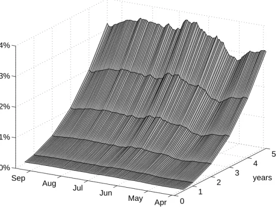
Figure 1 plots for each day in the sample the average term structure of default prob-abilities across the 125 firms. By definition, the term structures are upward sloping since
the probability of defaulting increases as maturity increases. Also, the graph shows that on average the first derivative with respect to maturity is increasing.12 Thus, forward default probabilities ∂Qt(τ≤s)
∂s , which measure the probability of defaulting at time s given that the
firm has not yet defaulted, are upward-sloping. Hence, the market expects the marginal probability of default to increase over time for the average firm. This is likely caused by the fact that the CDX NA IG index consists of solid investment grade firms with low short-term default probabilities, and it is therefore more probable that credit conditions worsen for a given firm than improve.
[Figure 1 about here.]
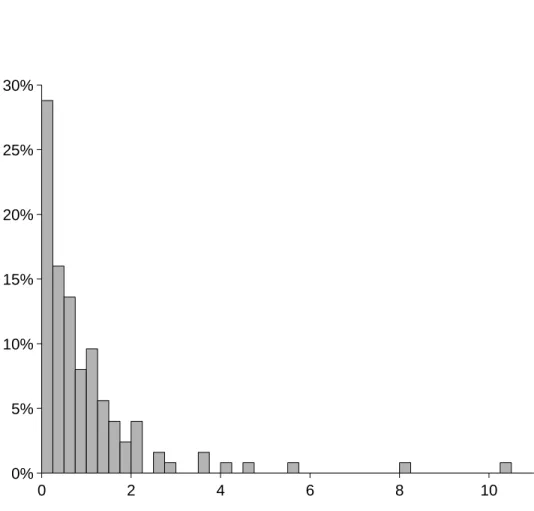
The sensitivity of each firm’s default probability to the economy-wide factor Y is cap-tured in the parameter ai, which is estimated model-independently through the covariance
between firm-specific instantaneous default probabilities and market-wide instantaneous de-fault probabilities. Figure 2 shows the distribution of ai’s across firms (remember that the
ai’s are normalized such that the average across firms is 1). There is a significant amount of
variation in the ai’s, and for a large fraction of the firms the default probabilities are quite
insensitive to market-wide fluctuations in credit risk. This suggests that the assumption in Duffie and Gˆarleanu (2001) to let all firms have the same sensitivity through identical ai’s
is not supported by the data.
[Figure 2 about here.]
To examine whether the subset of firms with large ai’s have common characteristics,
(11%), Financials (19%), Basic Industrials (23%), Telecommunications, Media and Technol-ogy (18%), Consumer Products and Retail (29%), and we find that firms with large ai’s are
fairly evenly distributed across these five sectors.13
The correlation between ai’s and the average 5-year CDS spread for firm i (averaging
across the 120 days) is 0.78 across the 125 firms. This strong positive correlation indicates that the ad hoc assumption in Mortensen (2006), Eckner (2007) and Eckner (2009), where
ai is exogenously set based on the firm-specific 5-year CDS spread, is reasonable.14
4.2
CDO Parameter Estimates and Pricing Results
The multi-name default model is estimated on the basis of a panel data set of daily CDS and CDO tranche spreads as described in section 2, and we assume that the measurement error matrix Σ in (9) is diagonal and use diffuse priors. We run the MCMC estimation routine
using a burn-in period of 20,000 simulations and a subsequent estimation period of another 10,000 simulations, where we use every 10th simulation to calculate parameter estimates.
The parameter estimates are given in Table 2, and the first thing we note is that the volatility of the common factor is σ = 0.0166, which is low compared to estimates in the previous literature: Duffee (1999) fits CIR processes to firm default intensities using corpo-rate bond data and finds an average σ of 0.074 and Eckner (2009) uses a panel data set of CDS and CDO spreads similar to the data set used here and estimates σ to be 0.103. An important factor in explaining this difference in the estimated size ofσ is the extent to which systematic and idiosyncratic default risk is separated. Duffee (1999) is not concerned with
such a subdivision of the default risk and therefore estimates a factor that includes both sys-tematic and unsyssys-tematic risk. Eckner (2009) has a model that is similar to ours, but when estimating the model he imposes strong restrictions on the parameters of the systematic and idiosyncratic factors. For example, he requires σ2 of the common factor to be equal to the average σ2
i of the idiosyncratic factors.
Our results suggest that separating default risk into an idiosyncratic and a common component, and letting these factors be fully flexible during the estimation, reveals that the common factor is ”slow-moving” in the sense that the volatility is low. In addition, we estimate the total contribution of jumpsl×µto be 6·10−5 which is lower than the estimate of 3·10−3in Eckner (2009), further underlining that the total volatility of the common factor is low when properly estimated.15 Finally, we note that although the common factor is not very volatile, it is explosive with a mean reversion coefficient of 0.94 under the risk-neutral measure. Under the actual measure, the factor is estimated to be mean-reverting, although the mean-reversion coefficient is hard to pin down with any precision due to the relatively short time span of our data sample.
[Table 2 about here.]
We now examine the pricing ability of our model by considering the average pricing errors and RMSEs (Root-Mean-Squared-Errors) given in Table 3. We see that on average the model underestimates spreads for the 3%−7% tranche by 7 basis points and overestimates the 10%−15% tranche by 4 basis points. For comparison, Mortensen (2006) reports average bid-ask spreads for the 3%−7% tranche to be 10.9 basis points and for the 10%−15% to
be 5 basis points. In both cases, average pricing errors are smaller than the bid-ask spread. The RMSEs of the model are larger than the average pricing errors, so the model errors are not consistently within the bid-ask spread, but RMSEs and pricing errors do suggest a good overall fit.
[Table 3 about here.]
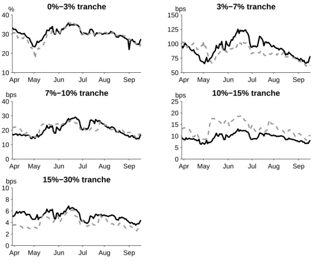
Figure 3 shows the observed and fitted CDO tranche spreads over time, and the graphs confirm a reasonable fit to all tranches apart from a slight underestimation of the 3%−7% tranche and overestimation of the 15%−30% tranche. It is particularly noteworthy that the time series variation in the most senior tranches – especially the 15%−30% tranche – is well matched. This is surprising because both the level and the time series variation of the 15%−30% tranche have been difficult to capture by models in the previous literature. Mortensen (2006) finds that jumps in the common factor are necessary to generate sufficiently high senior tranche spreads, but even with jumps it has been difficult to reproduce the observed time series variation in senior tranche spreads, as argued by Eckner (2009) and in a previous version of this paper.16 What enables our model to fit the time series variation of senior tranche spreads well is that we have not imposed the usual set of strong assumptions on the parameters of the common and idiosyncratic factors as done in Mortensen (2006), Eckner (2009), and in a previous version of this paper. Thus, a careful implementation of the multi-name default model frees up the model’s ability to fit tranche spreads in important dimensions.
To examine the contribution of systematic default risk to the total default risk across different maturities, we calculate the following: for each maturity, date, and firm we use the estimated sensitivitiesai and the path and parameters of the common factor Y to calculate
the systematic part of the risk-neutral default probability according to equation (1) and (2). We then find an average term-structure of systematic default risk by averaging across firms and dates and plot the result in Figure 4 together with the average total default risk inferred from observed CDS spreads. The figure shows that the systematic contribution to the overall default risk is small for short maturities but increases with maturity. As shown in Table 4 the average exposure to systematic default risk on a 6-month horizon is merely 0.003% and constitutes only 6% of the overall default risk, but increases to 0.874% and a fraction of 26% of the total default risk for a 5-year horizon. Hence, out of the total average 5-year default probability of 3.309%, 0.874% is systematic and non-diversifiable.
[Figure 4 about here.]
[Table 4 about here.]
5
Idiosyncratic Default Risk
So far in the estimation we have put structure on the systematic part of default risk through the specification of the common factor, while total default risk has been estimated model-independently. Combining the two elements gives us for each firm and each date a term structure of idiosyncratic default risk calculated as the “difference” between total default
risk and its systematic component.17 Thus, for each firm we have a data set consisting of the idiosyncratic part of the survival probability EtQ[exp(−Rt+s
t Xi,udu)] for maturities of s = 0.5,1,2,3,4,5 years for each of the 120 days in the sample. Given this panel data set we can now put structure on the idiosyncratic default risk and estimate the parameters of this structural form.
We can allow idiosyncratic default risk to be the sum of several factors and the factors can be of any distributional form subject only to the requirements of non-negativity and that we can calculate the expectation
EtQ exp − Z s t Xi,udu .
We choose to let the idiosyncratic factors have the same functional form as the common factor, namely be a one-factor affine jump-diffusion
dXi,t = (κi,0+κi,1Xi,t)dt+σi
p
Xi,tdWi,tQ+dJ Q i,t
with an essentially affine risk premium for diffusive risk and constant risk premium for the jump risk. This allows us to compare the results of our general estimation approach with those in previous literature, where a number of restrictions are placed jointly on the common and idiosyncratic factors. Thus, for each of the 125 firms in the sample, we estimate by MCMC the parameters of the idiosyncratic factor in the same way as the parameters of the common factor, but in this estimation we observe a panel data set of the idiosyncratic part of default probabilities instead of CDO prices. Note that structural assumptions on the idiosyncratic risk were not necessary in order to price CDOs in the previous section,
but adding structure here enables us to gain further understanding of the nature of the idiosyncratic default risk.
The results from the estimation of the idiosyncratic default factors are given in Table 5. We see that the average volatility across all firms isσ = 0.14, almost 10 times higher than the volatility estimate of 0.017 for the common factor. Combined with the parameter estimates discussed in the previous section, this shows that the idiosyncratic factors are more volatile than the systematic factor. The fact that the volatility of our systematic factor is lower than that reported in previous papers reflects that our estimation procedure allows us to fully separate the dynamics of the systematic factor from the dynamics of the idiosyncratic factors. This leads to a low-volatility systematic factor and high-volatility idiosyncratic factors, while previous research finds something in-between. In addition, we see that the average total (risk-neutral) contribution from jumps isl×µ= 4·10−2, which is higher than the total jump contribution in the systematic factor of 6·10−5, reinforcing the conclusion that volatilities of the idiosyncratic factors are higher than that of the systematic factor.
[Table 5 about here.]
We see thatκ1 is positive on average, so the idiosyncratic factors are on average explosive under the risk-neutral measure. However, they are less explosive than the systematic factor, implying that when pricing securities sensitive to default risk, the relative importance of systematic risk increases as maturity increases in accordance with our observations in Figure 4.
6
Conclusion
We present a new approach to estimate the relative contributions of systematic and idiosyn-cratic default risks in an intensity-based model. Based on a large data set of CDS and CDO tranche spreads on the North American Investment Grade CDX index, we find that our model is able to capture both the level and time series dynamics of CDO tranche spreads. We then go on and split the total default risk of a given entity into its idiosyncratic and systematic part. We find that the systematic default risk is explosive but has low volatility and that the relative contribution of systematic default risk is small for short maturities, but of growing importance as maturity increases. Our subsequent parametric estimation of the idiosyncratic default risks shows that idiosyncratic risk is more volatile and less explosive than systematic risk.
A
CDS Pricing
This section briefly explains how to price credit default swaps (CDSs). More thorough introductions are given in Duffie (1999) and O’Kane (2008).
A CDS contract is an insurance agreement between two counterparties written on the default event of a specific underlying reference obligation. The protection buyer pays fixed premium payments periodically until a default occurs or the contract expires, whichever happens first. If default occurs, the protection buyer delivers the reference obligation to the protection seller in exchange for face value.
For a CDS contract covering default risk between time t0 = t and tM = T and with
premium payment dates t1, . . . , tM, the value of the protection payment is given as
P rot(t, T) = EtQ (1−δ) exp − Z τ t rudu 1(τ≤T)
whereδis the recovery rate, while the value of the premium payment stream isS·P rem(t, T), where S is the annual CDS premium and
P rem(t, T) =EtQ " M X j=1 exp − Z min{tj,τ} t rudu ! Z tj tj−1 1(τ >s)ds # .
The CDS premium at time t is settled such that it equates the two payment streams, i.e.
S(t, T) = P remP rot((t,Tt,T)).
In order to calculate the CDS premiumS(t, T) we make the simplifying assumptions that the recovery rate δ is constant at 40%, that the riskfree interest rate is independent of the default timeτ, and finally that default, if it occurs, will occur halfway between two premium
payment dates. With these assumptions we can rewrite the two expressions above as P rot(t, T) = (1−δ) M X j=1 Pt,tj−1+tj 2 · Qt(τ > tj−1)−Qt(τ > tj) (10) P rem(t, T) = M X j=1 P t,tj−1+tj 2 ·tj−tj−1 2 · Qt(τ > tj−1)−Qt(τ > tj) + M X j=1 P(t, tj)· tj−tj−1 ·Qt(τ > tj). (11)
B
Calibration of Survival Probabilities
For the calibration of firm-specific survival probabilities from observed CDS spreads we assume that risk-neutral probabilities take the flexible form
Qt(τ > s) = 1 1 +α2+α4 e−α1(s−t)+α 2e−α3(s−t) 2 +α4e−α5(s−t) 3 s≥t (12)
with allαj ≥0. The calibrated survival probabilitiess 7→Qt(τ > s) for a given firm at time
t are then calculated by minimizing relative pricing errors using (10)–(12)
X T P rot(t, T) P rem(t, T) − Sobs(t, T) Sobs(t, T) !2
whereSobs(t, T) is the empirically observed CDS spread at timeton a contract with maturity
T. The calibration is based on observed CDS spreads for maturities of T = 0.5,1,2,3,4,5 years and is carried out separately for each firm, at each timet, and results in a very accurate fit to the observed CDS term structure.18
C
Estimation of Common Factor Sensitivities
The common factor sensitivities ai appearing in the specification (2) of individual default
intensities can be estimated by ordinary linear regression, and without exploiting specific assumptions on the dynamic evolution of the processes Y, X1, . . . , XN except for a mild
stationarity condition. As we argue in the following, this model-independent technique only relies on the availability of term structures of risk-neutral survival probabilities for each of the N issuers in the portfolio.
The simple idea that we build upon is the fact that (1) and (2) imply
−lim
s&0 ∂
∂sQt(τi > t+s) = λi,t =aiYt+Xi,t
and that we can calculate this quantity simply by inserting the calibrated survival probabil-ities on the left-hand-side of this expression.
If we now for fixed iconsider the regression
Wi,t =β0,i+β1,i(Vt−V¯) +εt t= 1, . . . , T where Wi,t =aiYt+Xi,t ¯ Wi = 1 T T X t=1 Wi,t Vt= 1 N N X j=1 Wj,t ¯ V = 1 T T X t=1 Vt
and εt is a Gaussian noise term, then it follows by standard estimation theory that ˆ β1,i = P t Wi,t−W¯i)(Vt−V¯ P t Vt−V¯ 2 .
Under the assumption of stationarity of each of the processes X1, . . . , XN, Y (and hence also
of Wi and V), we can rewrite the estimated regression coefficient as
ˆ β1,i = \ Cov(Wi, V) \ V ar(V) . (13)
Since X1, . . . , XN, Y are mutually independent then for sufficiently large N
Cov(Wi, V) = 1 NV ar(Xi) +aiV ar(Y)≈aiV ar(Y) (14) and similarly V ar(V) = 1 N2 N X j=1 V ar(Xj) +V ar(Y)≈V ar(Y) (15)
where we have applied the normalization N1 P
iai = 1. By combining (13), (14) and (15) it is
now straightforward to see that ˆβ1,i is an approximate estimator of the unknown sensitivity
ai.
To increase numerical robustness in the calculations, we make a small approximation and replace everywhere the instantaneous derivative
−lim
s&0 ∂
∂sQt(τi > t+s)
with the one-year default probability
1−Qt(τi > t+ 1) =−
Qt(τi > t+ 1)−Qt(τi > t)
1−0 ≈ −slim&0 ∂
since our calibration of the term structure of survival probabilities uses CDS contracts with maturities from 0.5 to 5 years, which results in minor numerical instabilities (across calendar time) in the very short end of the term structure.
D
Estimation of Common Factor
Once we have inferred marginal risk-neutral survival probabilities s 7→ qi,t(s) from CDS
spreads and estimated the common factors sensitivities ai, we are ready to estimate the
parameters and the path of the common factor processY. Throughout the estimation of the common factor process, all the qi,t(s) and all ai are taken as given (and thus held fixed).
Given an initial path of Y and initial values of the common factor parameters, the estimation procedure runs as follows:
(i) Calculate the common factor component of survival probabilities
EtQ −ai Z s t Yudu
for all firms i, all dates t and all maturities s.
(ii) Use the common factor componentsEtQ[(−ai
Rs
t Yudu)] from (i) and the calibrated term
structures of survival probabilitiesqi,t(s) to determine the idiosyncratic component of
survival probabilities EtQ − Z s t Xi,udu
for all firms i, all dates t and all maturities s using the relation
qi,t(s) =E Q t −ai Z s t Yudu ·EtQ − Z s t Xi,udu
(iii) Use the idiosyncratic components EtQ[(−Rs
t Xi,udu)] from (ii) as input to equation (5)
and calculate spreads for the 5 CDO tranches for all datest (this is what is referred to as the “pricing formula” f in section 2.2).
(iv) Use the MCMC estimation routine to update the parameters and the path of the common factorY, and repeat steps (i)-(iv) until convergence.
E
Conditional Posteriors in MCMC Estimation
In this Appendix the conditional posteriors stated in the main text and used in MCMC estimation are derived. Bayes’ rule
p(X|Y)∝p(Y|X)p(X)
is repeatedly used in the calculations.
E.1
Conditionals of
S, Y, J
, and
Z
The conditional posteriors of S, Y, J, and Z are used in most of the conditional posteriors for the parameters and are therefore derived in this section.
E.1.1 p(Y|Θ,Σ, J, Z) and p(S|Θ,Σ, Y, J, Z)
With the discretization in (8) we have that
p(Y|Θ,Σ, J, Z) = YT t=1 p(Yt|Yt−1,Θ,Σ, J, Z) p(Y0) = p(Y0) T Y t=1 1 σ√∆tYt−1 exp−1 2 [Yt−(κ0∆t+ (κP1∆t+ 1)Yt−1+JtZt)]2 σ2∆ tYt−1 ∝ p(Y0)σ−TY −1 2 x exp − 1 2 T X t=1 [Yt−(κ0∆t+ (κP1∆t+ 1)Yt−1+JtZt)]2 σ2∆ tYt−1 (16)
whereYx =QTt=1Yt−1. Note that the posteriorp(Y|Θ,Σ, J, Z) differs fromp(Y|Θ,Σ, J, Z, S).
The conditional posterior of S is found as
p(S|Θ,Σ, Y, J, Z) = T Y t=1 |Σ|− 1 2 exp −1 2[St−f(Θ Q, Y t)]0Σ−1[St−f(ΘQ, Yt)] = |Σ|− T 2 exp − 1 2 T X t=1 ˆ e0tΣ−1ˆet) , (17)
where ˆet=St−f(ΘQ, Yt). If Σ is diagonal this simplifies to
p(S|Θ,Σ, Y, J, Z)∝ N Y i=1 Σ− T 2 ,ii exp − 1 2Σ,ii T X t=1 ˆ e2t,i.
This posterior does not depend on J, Z, κP
E.1.2 p(Z|Θ,Σ, Y, J, S) and p(J|Θ,Σ, Y, Z, S)
Since Zt is exponentially distributed we have that
p(Z|Θ,Σ, Y, J, S) ∝ p(S|Θ,Σ, Y, J, Z)p(Z|Θ,Σ, Y, J) (18) ∝ p(Y|Θ,Σ, J, Z)p(Z|Θ,Σ, J) ∝ p(Y|Θ,Σ, J, Z) T Y t=1 1 µP exp(− Zt µP) ∝ p(Y|Θ,Σ, J, Z)(µP)−T exp(− Z• µP) (19) where Z• =PTt=1Zt.
The jump time Jt can only take on two values so the conditional posterior for Jt is
Bernoulli. The Bernoulli probabilities are given as
p(J|Θ,Σ, Y, Z, S) ∝ p(S|Θ,Σ, Y, J, Z)p(J|Θ,Σ, Y, Z) (20) ∝ p(Y|Θ,Σ, J, Z)p(J|Θ,Σ, Z) ∝ p(Y|Θ,Σ, J, Z)p(J|Θ) ∝ p(Y|Θ,Σ, J, Z) T Y t=1 (lP∆t)Jt(1−lP∆t)1−Jt ∝ p(Y|Θ,Σ, J, Z)(lP∆t)J•(1−lP∆t)T−J• (21) with J• =PTt=1Jt
E.2
Conditional Posteriors
The conditional posteriors are derived and the choice of priors for the posteriors are discussed in this section.
(i) The conditional posterior of the error matrix Σ is given as
p(Σ|Θ, Y, J, Z, S) ∝ p(S|Θ,Σ, Y, J, Z)p(Σ|Θ, Y, J, Z) ∝ p(S|Θ,Σ, Y, J, Z)p(Σ|Θ) ∝ |Σ|− T 2 exp −1 2 T X t=1 ˆ e0tΣ−1eˆt p(Σ|Θ) = |Σ|− T 2 exp −1 2tr(Σ −1 T X t=1 ˆ etˆe0t) p(Σ|Θ).
The last line follows because−1 2 PT t=1ˆe 0 tΣ −1 ˆet=−12PTt=1tr(ˆe0tΣ −1 eˆt) = −12PTt=1tr(Σ−1eˆteˆ0t) = −1 2tr( PT t=1Σ −1 eˆteˆ0t) = −12tr(Σ −1 PT
t=1ˆeteˆ0t). If the prior on Σ is independent of the
other parameters and has an inverse Wishart distribution with parameters V and m
thenp(Σ|...) is inverse Wishart distributed with parametersV +PTt=1eˆteˆ0tandT +m.
The special case ofV equal to the zero matrix and m= 0 corresponds to a flat prior.
(ii) The conditional posterior ofκP
1 is found as p(κP1|Θ\κP 1,Σ, Y, J, Z, S) ∝ p(S|Θ,Σ, Y, J, Z)p(κ P 1|Θ\κP 1,Σ, Y, J, Z) ∝ p(κP1|Θ\κP 1,Σ, Y, J, Z) ∝ p(Y|Θ,Σ, J, Z)p(κP1|Θ\κP 1,Σ).
According to equation (16) we have
p(κP1|...)∝exp− 1 2 T X t=1 [Yt−(κ0∆t+ (κP1∆t+ 1)Yt−1+JtZt)]2 σ2∆ tYt−1 p(κP1|Θ\κP 1,Σ)
so p(κP1|...)∝exp− 1 2 T X t=1 [atκP1 −bt]2 σ2∆ tYt−1 p(κP1|Θ\κP 1,Σ) where at = −∆tYt−1 bt = κ0∆t+Yt−1+JtZt−Yt.
Using the result in Fr¨uhwirth-Schnatter and Geyer (1998, p. 10) and assuming flat priors we have that κP
1 ∼N(Qm, Q) where m = T X t=1 atbt σ2∆ tYt−1 Q−1 = T X t=1 a2 t σ2∆ tYt−1 .
(iii) For the jump size parameter µP the conditional posterior is found as
p(µP|Θ\µP,Σ, Y, J, Z, S) ∝ p(S|Θ,Σ, Y, J, Z)p(µP|Θ\µP,Σ, Y, J, Z) ∝ p(Y|Θ,Σ, J, Z)p(µP|Θ\µP,Σ, J, Z) ∝ p(Z|Θ,Σ, J)p(µP|Θ\µP,Σ, J) ∝ p(Z|Θ)p(µP|Θ\µP,Σ) ∝ (µP)−T exp(−Z• µP)p(µ P|Θ \µP,Σ).
If the prior onµP is flat then the conditional posterior inverse gamma distributed with
(iv) The same calculations as for the jump-size parameter µP yields the conditional
poste-rior of the jump-time parameter lP as
p(lP|Θ\lP,Σ, Y, J, Z, S) ∝ p(J|Θ)p(lP|Θ\lP,Σ)
∝ (lP∆t)J•(1−lP∆t)T−J•
p(lP|Θ\lP,Σ).
Assuming a flat prior onlP the conditional posterior oflP∆
tis beta distributed,lP∆t∼ B(J•+ 1, T −J•+ 1).
(v) The parameters σ and κ0 are sampled by Metropolis-Hastings since the conditional distributions are not known. Denoting any of the two parameters θi, the conditional
distribution is found as
p(θi|Θ\θi,Σ, Y, J, Z, S) ∝ p(S|Θ,Σ, Y, J, Z)p(θi|Θ\θi,Σ, Y, J, Z)
∝ p(S|Θ,Σ, Y, J, Z)p(Y|Θ,Σ, J, Z)p(θi|Θ\θi,Σ, J, Z)
∝ p(S|Θ,Σ, Y, J, Z)p(Y|Θ,Σ, J, Z)p(θi|Θ\θi,Σ).
Flat priors on both parameters are assumed.
(vi) The parameters κQ1, lQ, and µQ are sampled by Metropolis-Hastings. The only
dif-ference in the derivation of their conditional distributions compared to derivation of the distributions of σ and κ0 is that the distribution of Y does not depend on these three parameters. Letting θi represent any of the three parameters, the conditional
distribution is found as
p(θi|Θ\θi,Σ, Y, J, Z, S) ∝ p(S|Θ,Σ, Y, J, Z)p(θi|Θ\θi,Σ, Y, J, Z)
∝ p(S|Θ,Σ, Y, J, Z)p(Y|Θ,Σ, J, Z)p(θi|Θ\θi,Σ, J, Z)
∝ p(S|Θ,Σ, Y, J, Z)p(θi|Θ\θi,Σ).
Flat priors on all three parameters are assumed.
(vii) The latent jump indicators Jt’s are sampled individually from Bernoulli distributions.
To see this, note that equation (21) implies that
p(J|Θ,Σ, Y, Z, S) ∝ T Y t=1 exp− 1 2 [Yt−(κ0∆t+ (κP1∆t+ 1)Yt−1+JtZt)]2 σ2∆ tYt−1 lP∆t 1−lP∆ t Jt .
In the actual implementation we use
p(J|Θ,Σ, Y, Z, S) ∝ T Y t=1 exp −1 2 (−2[Yt−(κ0∆t+ (κP1∆t+ 1)Yt−1)] +JtZt)JtZt σ2∆ tYt−1 lP∆t 1−lP∆ t Jt
since this is numerically more robust.
(viii) For the latent jump sizesZt we have according to equation (19) that
p(Z|Θ,Σ, Y, J, S) ∝ T Y t=1 exp− 1 2 [Yt−(κ0∆t+ (κP1∆t+ 1)Yt−1+JtZt)]2 σ2∆ tYt−1 − Zt µP
so the Zts are conditionally independent and are sampled individually. If Jt = 0
calculations show that p(Zt|Θ,Σ, Y, J, Z\Zt, S)∝ [((κP 1 +µPσ2)∆t+ 1)Yt−1−(Yt−κ0∆t) +Zt]2 σ2∆ tYt−1 ,
where Zt ≥ 0. Therefore, Zt is drawn from a N((Yt− κ0∆t)− ((κP1 +µPσ2)∆t+
1)Yt−1, σ2∆tYt−1) distribution and the draw is rejected if Zt < 0. In practice the
number of rejections are small.19
(ix) The latent Yts are sampled individually by Metropolis-Hastings and fort= 1, ..., T−1
the conditional posterior is
p(Yt|Θ,Σ, Y\Yt, J, Z, S) ∝ p(S|Θ,Σ, Y, J, Z, S)p(Yt|Θ,Σ, Y\Yt, J, Z)
∝ p(St|Θ,Σ, Yt, J, Z, S)p(Yt|Θ,Σ, Yt−1, Yt+1, J, Z)
∝ p(St|Θ,Σ, Yt, J, Z, S)
×p(Yt|Θ,Σ, Yt−1, J, Z)p(Yt+1|Θ,Σ, Yt, J, Z)
ForYT the conditional posterior is
p(YT|Θ,Σ, Y\YT, J, Z, S) ∝ p(YT|Θ,Σ, YT−1, J, Z, S)
∝ p(ST|Θ,Σ, YT, J, Z, S)p(YT|Θ,Σ, YT−1, J, Z)
while for Y0 it is
p(Y0|Θ,Σ, Y\Y0, J, Z, S) ∝ p(Y0|Θ,Σ, Y1, J, Z)
E.3
Implementation Details
In the RW-MH steps of the MCMC sample, the proposal density is chosen to be Gaussian, and the efficiency of the RW-MH algorithm depends crucially on the variance of the proposal normal distribution. If the variance is too low, the Markov chain will accept nearly every draw and converge very slowly while it will reject a too high portion of the draws if the variance is too high. We therefore do an algorithm calibration and adjust the variance in the first half of the burn-in period in the MCMC algorithm. Roberts et al. (1997) recommend acceptance rates close to 14 and therefore the standard deviation during the algorithm calibration is chosen as follows: Every 100’th draw the acceptance ratio of each parameter is evaluated. If it is less than 10 % the standard deviation is doubled while if it is more than 50 % it is cut in half. This step is prior to the second half of the burn-in period since the convergence results of RW-MH only applies if the variance is constant (otherwise the Markov property of the chain is lost).
The Fourier inversion in equation (7) is calculated by using Fast Fourier Transform and the number of points used in FFT is 218. We use Simpson’s rule in the Fast Fourier Transform routine as suggested by Carr and Madan (1999), and our results suggest a significant im-provement in overall accuracy. The characteristic function is not evaluated in every Fourier transform point. Instead, since the characteristic function is exponential-affine with func-tion Aand B, the functions A and B are splined from a lower number of points. The spline uses a total number of 60 points. Also, the integration in (6) is done using Gauss-Legendre integration and the number of integration points is 60.
Notes
1Examples of empirical applications are Duffie and Singleton (1997), Duffee (1999), and Longstaff, Mithal, and Neis (2005).
2To illustrate why the Feller condition is necessary in extended affine models consider the simple diffusion case,dYt= (κQ0 +κ
Q
1Yt)dt+σ
√
YtdWQ. The risk premium Λt= √λY0
t+λ1 √
Ytkeeps the process affine under
P but the risk premium explodes if Yt= 0. To avoid this, the Feller restrictionκ0> σ
2
2 under bothP and
Qensures thatYt is strictly positive.
3The last term disappears ifj= 0.
4Duffie and Gˆarleanu (2001) derive an explicit solution forEQ t [exp(q
Rs
t Yudu)] whenqis a real number,
but as noted by Eckner (2009) the formula works equally well forqcomplex. 5Pricing CDS contracts is explained in Appendix A.
6For a general introduction to MCMC see Robert and Casella (2004) and for a survey of MCMC methods in financial econometrics see Johannes and Polson (2006).
7This procedure is essentially similar to the well-known technique for inferring a term structure of interest rates from observed prices of coupon bonds, see Nelson and Siegel (1987).
8The average of thea0
is are without loss of generality normalized to 1.
9All random numbers in the estimation are draws from Matlab 7.0’s generator which is based on Marsaglia and Zaman (1991)’s algorithm. The generator has a period of almost 21430 and therefore the number of random draws in the estimation is not anywhere near the period of the random number generator.
10Upfront payments may be converted to running spreads using so-called “risky duration”, see e.g. Amato and Gyntelberg (2005). This calculation requires a fully parametric model, and hence is not possible within our modelling framework. Instead we use the original upfront payment quotes available from MarkIt for the equity tranche.
11The 5-year CDS contracts for the period March 21, 2006 to June 19, 2006 mature on June 20, 2011, consistent with the maturity of the 5-year CDO tranches, but for the period June 20 to September 19, 2006,
the maturity of the 5-year CDS contracts is September 20, 2011 (and the maturity of the other CDS contracts are similarly shifted forward by 3 months from June 20 and onwards). However, this maturity mismatch between the CDS and CDO contracts in the latter part of our sample period is automatically corrected for, when we imply out the term structures of firm-specific survival probabilities from observed CDS spreads (see appendix B), and hence poses no problem to the estimation of the model.
12This observation is apparent from a visual inspection of the graph, and quantitative estimates are available upon request.
13The distribution on sectors of the firms with the 20% largest market sensitivities a
i is: Energy (8%),
Financials (8%), Basic Industrials (16%), Telecommunications, Media and Technology (28%), Consumer Products and Retail (40%).
14Mortensen (2006) fixesa
i implicitly through a parameter restriction but notes that it effectively
corre-sponds to settingai equal to the fraction of firm-specific to average (across all firms) 5-year CDS spread.
15In a previous version of this paper, we imposed parameter restrictions similar to Eckner (2009), which resulted in parameter estimates consistent with those that he reports.
16The previous version of the paper entitled ”An empirical investigation of an intensity-based model for pricing CDO tranches” is available upon request.
17More specifically, the relation
Qt(τi> s) =E Q t −ai Z s t Yudu ·EtQ − Z s t Xi,udu
allows us to infer the idiosyncratic part of survival probabilities directly from the estimated common factor and the CDS implied survival probabilities,EtQ
−ai
Rs
t Yudu
andQt(τi> s) respectively.
18This calibration approach is close to the industry benchmark of fitting the observed CDS term structure perfectly using piecewise constant intensities, see O’Kane (2008).
Figure legends
Figure 1. Default probabilities. The figure shows the average calibrated term structure of risk-neutral default probabilities for 0 to 5 years over the period March 30, 2006 to September 20, 2006, averaging across all 125 constituents of the CDX NA IG 6 index. Default probabilities are calibrated on a firm-by-firm basis following the procedure outlined in appendix B.
Figure 2. Common factor sensitivities. The figure shows the distribution of the estimated common factor sensitivitiesaifor the 125 constituents of the CDX NA IG 6 index. The sensitivities are estimated following
the procedure outlined in appendix C.
Figure 3. CDO tranche spreads. The graphs show the observed (solid black) and model-implied (dashed gray) CDO tranche spreads for the five CDX NA IG 6 tranches: 0%−3%, 3%−7%, 7%−10%, 10%−15%, and 15%−30% over the period March 30, 2006 to September 20, 2006. The model-implied spreads are based on the parameter estimates reported in Table 2.
Figure 4. Average default probabilities. The figure shows the average term structure of risk-neutral default
probabilities, averaging across all 125 constituents of the CDX NA IG 6 index and across all trading days in the period March 30, 2006 to September 20, 2006. The default probabilities are decomposed into their common (dark gray) and idiosyncratic (light gray) parts. The total default probabilities (dark and light gray) are calibrated from CDS spreads (see appendix B), and the common part is calculated using the parameter estimates reported in Table 2.
References
Amato, J. D. and J. Gyntelberg (2005). CDS Index Tranches and the Pricing of Credit Risk Correlations. BIS Quarterly Review, March, 73–87.
Andersen, L., J. Sidenius, and S. Basu (2003, November). All Your Hedges in One Basket.
Risk, 67–72.
Besag, J. (1974). Spatial Interaction and the Statistical Analysis of Lattice Systems. Jour-nal of the Royal Statistical Association Series B 36, 192–236.
BIS (2007). Triennial Central Bank Survey.Bank for International Settlements.
Campbell, J. Y. and G. B. Taksler (2003). Equity Volatility and Corporate Bond Yields.
Journal of Finance 58, 2321–2349.
Carr, P. and D. B. Madan (1999). Option Valuation Using the Fast Fourier Transform.
Journal of Computational Finance 2, 61–73.
Cheridito, P., D. Filipovic, and R. L. Kimmel (2007). Market Price of Risk Specifications for Affine Models: Theory and Evidence.Journal of Financial Economics 83, 123–170. Collin-Dufresne, P. (2009). A Short Introduction to Correlation Markets. Journal of
Fi-nancial Econometrics 7, 12–29.
Duffee, G. (1999). Estimating the Price of Default Risk.Review of Financial Studies 12, 197–226.
Duffie, D. (2008). Innovations in Credit Risk Transfer: Implications for Financial Stability.
BIS Working Paper No. 255.
Duffie, D. and N. Gˆarleanu (2001). Risk and Valuation of Collateralized Debt Obligations.
Financial Analysts Journal 57(1), 41–59.
Duffie, D. and K. Singleton (1997). An Econometric Model of the Term Structure of Interest Rate Swap Yields. Journal of Finance 52, 1287–1321.
Duffie, D. and K. J. Singleton (1999). Modeling Term Structures of Defaultable Bonds.
Review of Financial Studies 12, 687–720.
Eckner, A. (2007). Risk Premia in Structured Credit Derivatives. Working Paper, Stan-ford.
Eckner, A. (2009). Computational Techniques for Basic Affine Models of Portfolio Credit Risk. Journal of Computational Finance 13, 63–97.
Errais, E., K. Giesecke, and L. R. Goldberg (2010). Affine point processes and portfolio credit risk.SIAM Journal of Financial Mathematics 1, 642–665.
Feldh¨utter, P. (2006). Can Affine Models Match the Moments in Bond Yields? Working Paper, Copenhagen Business School.
Feldh¨utter, P. and D. Lando (2008). Decomposing Swap Spreads. Journal of Financial Economics 88, 375–405.
Fr¨uhwirth-Schnatter, S. and A. L. Geyer (1998). Bayesian Estimation of Econometric Mul-tifactor Cox Ingersoll Ross Models of the Term Structure of Interest Rates via MCMC
Methods. Working Paper, Department of Statistics, Vienna University of Economics and Business Administration.
Gelfand, A. E., A. F. Smith, and T.-M. Lee (1992). Bayesian Analysis of Constrained Pa-rameter and Truncated Data Problems Using Gibbs Sampling.Journal of the American Statistical Association 87, 523–532.
Geman, S. and D. Geman (1984). Stochastic Relaxation, Gibbs Distributions and the Bayesian Restoration of Images.IEEE Trans. on Pattern Analysis and Machine Intel-ligence 6, 721–741.
Giesecke, K., L. R. Goldberg, and X. Ding (2011). A Top-Down Approach to Multiname Credit.Operations Research 59, 283–300.
Hammersley, J. and P. Clifford (1970). Markov Fields on Finite Graphs and Lattices.
Unpublished Manuscript.
Johannes, M. and N. Polson (2006). MCMC Methods for Financial Econometrics. Hand-book of Financial Econometrics (Chapter).
Lando, D. (1994). Three Essays on Contingent Claims Pricing. Ph. D. thesis, Cornell University.
Longstaff, F., S. Mithal, and E. Neis (2005). Corporate Yield Spreads: Default Risk or Liquidity? New Evidence from the Credit Default Swap Market.Journal of Finance 60, 2213–2253.
Debt Obligations. Journal of Finance 63, 529–563.
Marsaglia, G. and A. Zaman (1991). A New Class of Random Number Generators.Annals of Applied Probability 3, 462–480.
Metropolis, N., A. Rosenbluth, M. Rosenbluth, A. Teller, and E. Teller (1953). Equations of State Calculations by Fast Computing Machines. Journal of Chemical Physics 21, 1087–1091.
Mortensen, A. (2006). Semi-Analytical Valuation of Basket Credit Derivatives in Intensity-Based Models. Journal of Derivatives, 8–26.
Nelson, C. R. and A. F. Siegel (1987). Parsimonious Modeling of Yield Curves. Journal of Business 60, 473–489.
O’Kane, D. (2008).Modelling Single-Name and Multi-Name Credit Derivatives. Wiley. Robert, C. P. and G. Casella (2004). Monte Carlo Statistical Methods (2 ed.).
Springer-Verlag.
Roberts, G., A. Gelman, and W. Gilks (1997). Weak Convergence and Optimal Scaling of Random Walk Metropolis Algorithms. Annals of Applied Probability 7, 110–120. Zhang, B. Y., H. Zhou, and H. Zhu (2009). Explaining Credit Default Swap Spreads
with the Equity Volatility and Jump Risks of Individual Firms. Review of Financial Studies 22, 5099–5131.
Figures
0 1 2 3 4 5 Apr May Jun Jul Aug Sep 0% 1% 2% 3% 4% yearsFigure 1. Default probabilities. The figure shows the average calibrated term structure of risk-neutral default probabilities for 0 to 5 years over the period March 30, 2006 to September 20, 2006, averaging across all 125 constituents of the CDX NA IG 6 index. Default probabilities are calibrated on a firm-by-firm basis following the procedure outlined in appendix B.
0 2 4 6 8 10 0% 5% 10% 15% 20% 25% 30%
Figure 2. Common factor sensitivities. The figure shows the distribution of the estimated common factor sensitivitiesai for the 125 constituents of the CDX NA IG 6 index. The sensitivities are estimated
Apr May Jun Jul Aug Sep 10 20 30 40 0%−3% tranche %
Apr May Jun Jul Aug Sep
50 75 100 125 150 3%−7% tranche bps
Apr May Jun Jul Aug Sep
0 10 20 30 40 7%−10% tranche bps
Apr May Jun Jul Aug Sep
0 5 10 15 20 25 10%−15% tranche bps
Apr May Jun Jul Aug Sep
0 2 4 6 8 10 15%−30% tranche bps
Figure 3. CDO tranche spreads. The graphs show the observed (solid black) and model-implied (dashed gray) CDO tranche spreads for the five CDX NA IG 6 tranches: 0%−3%, 3%−7%, 7%−10%,
10%−15%, and 15%−30% over the period March 30, 2006 to September 20, 2006. The model-implied spreads are based on the parameter estimates reported in Table 2.
0 1 2 3 4 5 0% 1% 2% 3% 4% years common idiosyncratic
Figure 4. Average default probabilities. The figure shows the average term structure of risk-neutral default probabilities, averaging across all 125 constituents of the CDX NA IG 6 index and across all trading days in the period March 30, 2006 to September 20, 2006. The default probabilities are decomposed into their common (dark gray) and idiosyncratic (light gray) parts. The total default probabilities (dark and light gray) are calibrated from CDS spreads (see appendix B), and the common part is calculated using the parameter estimates reported in Table 2.
Tables
Panel A: CDS spreads for CDX NA IG 6 constituents
Maturity 0.5 yr 1 yr 2 yrs 3 yrs 4 yrs 5 yrs
(in bps) (in bps) (in bps) (in bps) (in bps) (in bps)
Mean 6.78 8.75 14.58 21.52 30.52 39.14 Std. 5.77 6.62 11.25 16.74 23.44 29.82 Median 4.86 6.56 10.72 16.07 22.51 29.03 Min. 0.41 1.73 2.65 2.94 3.99 5.45 Max. 56.46 59.82 103.73 140.48 181.60 222.19 Observations 15,000 15,000 15,000 15,000 15,000 15,000
Panel B: CDO tranche spreads for CDX NA IG 6 tranches
Tranche 0%−3% 3%−7% 7%−10% 10%−15% 15%−30%
(in %) (in bps) (in bps) (in bps) (in bps)
Mean 29.95 91.83 20.43 9.33 5.13 Std. 2.92 15.37 4.27 1.58 0.74 Median 30.29 92.48 20.31 9.06 5.17 Min. 21.97 65.52 13.96 6.40 3.54 Max. 35.75 125.02 28.97 13.02 6.84 Observations 120 120 120 120 120
Table 1. Summary statistics. Panel A reports summary statistics for CDS spreads of the 125 constituents of the CDX NA IG 6 index over the period March 30, 2006 to September 20, 2006. Panel B reports summary statistics for the five CDO tranches: 0%−3%, 3%−7%, 7%−10%, 10%−15%, and 15%−30% of the CDX NA IG 6 index over the same period.