econ
stor
www.econstor.eu
Der Open-Access-Publikationsserver der ZBW – Leibniz-Informationszentrum Wirtschaft
The Open Access Publication Server of the ZBW – Leibniz Information Centre for Economics
Nutzungsbedingungen:
Die ZBW räumt Ihnen als Nutzerin/Nutzer das unentgeltliche, räumlich unbeschränkte und zeitlich auf die Dauer des Schutzrechts beschränkte einfache Recht ein, das ausgewählte Werk im Rahmen der unter
→ http://www.econstor.eu/dspace/Nutzungsbedingungen nachzulesenden vollständigen Nutzungsbedingungen zu vervielfältigen, mit denen die Nutzerin/der Nutzer sich durch die erste Nutzung einverstanden erklärt.
Terms of use:
The ZBW grants you, the user, the non-exclusive right to use the selected work free of charge, territorially unrestricted and within the time limit of the term of the property rights according to the terms specified at
→ http://www.econstor.eu/dspace/Nutzungsbedingungen By the first use of the selected work the user agrees and declares to comply with these terms of use.
Xu, Fang
Working Paper
Does Consumption-Wealth Ratio Signal
Stock Returns? : VECM Results for
Germany
Economics working paper / Christian-Albrechts-Universität Kiel, Department of Economics, No. 2005,02
Provided in cooperation with:
Christian-Albrechts-Universität Kiel (CAU)
Suggested citation: Xu, Fang (2005) : Does Consumption-Wealth Ratio Signal Stock Returns? : VECM Results for Germany, Economics working paper / Christian-Albrechts-Universität Kiel, Department of Economics, No. 2005,02, http://hdl.handle.net/10419/21989
Economics Working Paper
No 2005-02
Does Consumption-Wealth Ratio Signal Stock
Returns? - VECM Results for Germany
Does Consumption-Wealth Ratio Signal Stock
Returns? - VECM Results for Germany
Fang Xu
∗Christian-Albrechts-University of Kiel
March 2005
Abstract
This paper studies the signalling effect of the consumption-wealth ratio (cay) on Ger-man stock returns via vector error correction models (VECMs). The effect of cay on U.S. stock returns has been recently confirmed by Lettau and Ludvigson with a two-stage method. In this paper, performances of the VECMs and the two-two-stage method are compared in both German and U.S. data sets. It is found that the VECMs are more suitable to study the effect of cay on stock returns than the two-stage method. Using the Conditional-Subset VECM,caysignals real stock returns and excess returns in both data sets significantly. The estimated coefficient oncay for stock returns turns out to be two times greater in U.S. data than in German data. When the two-stage method is used, cay has no significant effect on German stock returns. Besides, it is also found that cay signals German wealth growth and U.S. income growth signifi-cantly.
Keywords: stock returns, consumption-wealth ratio, VECM JEL Classification: C32, G10
1
Introduction
Since the 1990s, there is evidence that stock returns could be signalled by macro-economic variables, such as the investment-capital ratio (Cochrane 1991) and the consumption-wealth ratio (Lettau & Ludvigson 2001). Using U.S. quarterly data from 1952 to 1998, Lettau and Ludvigson find that consumption, asset holdings, and labor
∗Institute for Statistics and Econometrics, Christian-Albrechts-University of Kiel, Olshausenstr.
40-60, D-24118 Kiel, Germany, fangxu@stat-econ.uni-kiel.de. The author is grateful to Helmut Herwartz, Harald Uhlig, Monique Ebell, and Hans-Eggert Reimers.
income are cointegrated. The deviations from the common trend, the consumption-wealth ratio, is a strong signal of stock returns, but not of consumption growth. This evidence is interpreted by the forward-looking behaviour of investors. When the future stock returns are expected to increase (decrease), the investor who want to smooth the consumption path will increase (decrease) the consumption above (under) its trend with the current wealth and labor income. A two-stage method has been used by Lettau and Ludvigson. In the first stage, the dynamic least square (DLS) approach is adopted to estimate the regression of consumption on wealth and labor income. Using the estimated coefficients, the estimated trend deviation,dcay, can be obtained. In the second stage, the signalling effect ofdcay on stock returns is investigated via the ordinary least squares (OLS) regression or the vector autoregressive (VAR) model.
This paper studies the role of cay as a signal of German stock returns in the vector error correction models (VECMs). Not only the signalling effect of cay on stock returns but also the cointegration relation among consumption, wealth and labor income can be investigated via the VECMs in one stage. To compare the performance of the two-stage method with the one of the VECMs, both Germany and U.S. data sets have been investigated. U.S. quarterly data from 1952.4 to 1998.3 are those from Lettau and Ludvigson (2001). German quarterly data are from 1971.1 to 2002.4. It turns out that the VECMs provide a more efficient way to analyze the relation among consumption, wealth, labor income, and stock returns. Using the Conditional-Subset VECM,cay signals both real stock returns and excess return over a Treasury bill rate in both German and U.S. data sets significantly. When the two-stage method is used, the effect of cay on stock returns is not confirmed in German data. Moreover, via the Conditional-Subset VECM,cay has significant impact on German wealth growth and U.S. income growth. These empirical results cannot be explained by the theory of the consumption-wealth ratio.
The rest of the paper is organized as follows. Part 2 presents the macroeconomic model of the consumption-wealth ratio. Part 3 describes the VECMs used in this paper and the two-stage method used by Lettau and Ludvigson. Part 4 shows the performance ofcayin the German data with the two-stage method. Part 5 investigates the signalling effect of cay on stock returns in both data sets with the VECMs. Part 6 concludes.
2
The Consumption-Wealth Ratio
Consider the intertemporal budget constraint of a consumer who invests the wealth in a single asset with a time-varing risky return. In this representative agent economy all wealth, including human capital, is tradable. The two-period budget constraint is,
Wt+1 = (1 +Rw,t+1)(Wt−Ct), (1)
where Wt denotes the aggregate wealth in period t and Rw,t+1 is the net return on
the invested aggregate wealth. The invested aggregate wealth is the subtraction of consumption Ct from the aggregate wealth Wt. Campbell and Mankiw (1989) show
log version, and solving the resulting function forward, the log consumption-wealth ratio can be obtained as,
ct−wt= ∞ X i=1 ρi w(rw,t+i−∆ct+i) +ρk/(1−ρ). (2)
The lowercase letters denote log variables of the corresponding uppercase letters throughout. ρandkare constant terms. Equation (2) shows that the log consumption-wealth ratio of today is associated with the future rate of return on invested consumption-wealth and future consumption growth.
Four further assumptions for the consumption-wealth ratio have been made by Lettau and Ludvigson (2001). First, they consider equation (2) to be held ex ante. Second, they assume that the wealth Wt is the sum of asset holdings At and
hu-man capital Ht, Wt = At +Ht. The log aggregate wealth may be represented as,
wt ≈ωat+ (1−ω)ht, where ω is the average ratio of asset holdings to total wealth,
A/W. The lowercase letters denote log variables of the corresponding uppercase let-ters throughout. Third, it is assumed that the observable aggregate labor income,Yt,
can describe the unobservable human capital, Ht. Thus, ht = κ+yt+zt, where κ
is a constant and zt is a mean zero stationary random variable. Finally, Lettau and
Ludvigson assume that log consumption is a constant multiple of log nondurables and services,
ct =λcn,t, (3)
where λ >1 and cn,t denotes log nondurable consumption. Based on these
assump-tions, the log consumption-wealth ratio may be written as,
cn,t−βaat−βyyt = (1/λ)Et ∞ X i=1 ρiw{[ωra,t+i+ (1−ω)rh,t+i]−∆ct+i} +(1/λ)(1−ω)zt, (4)
where βa = (1/λ)ω and βy = (1/λ)(1−ω). βa+βy identifies 1/λ, which is smaller
than 1. ra denotes the logarithm of the gross return on the asset holdings and rh the
logarithm of the gross return on human capital. Et is the conditional expectation on
information available at time t. The constant term is omitted here because it does not play a role in the analysis. Since all the variables on the right-hand side of (4) are presumed stationary, the variables on the left-hand side, cn,t, at, and yt, might
be cointegrated. The deviation from the common trend, the log consumption-wealth ratio, is obtained as, cayt = cn,t−βaat−βyyt. According to this relation, cayt can
signal the expected return on future assets if the expected return on human capital,
rh,t+i, and the expected consumption growth, ∆ct+i, are not too volatile or these
variables are strongly correlated with the expected return on asset, ra,t+i.
3
Methodology
This section describes two different methods which are used to investigate the per-formance of cay. Both of these methods are based on the evidence that nondurables
consumption, household net worth (measure of asset holdings), and labor income all contain a unit root and there is a single cointegrating vector for these three variables.
3.1
Two-Stage Method
In the first stage, to estimate the cointegrating vector, βa and βy in equation (4),
Lettau and Ludvigson (2001) use a dynamic least squares (DLS) technique (Stock & Watson 1993). The DLS specification takes the form,
cn,t =α+βaat+βyyt+ k X i=−k ba,i∆at−i+ k X i=−k by,i∆yt−i+²t, (5)
where ∆ is the first difference operator, e.g. ∆yt =yt−yt−1. Based on the standard
OLS estimation of equation (5), the estimated trend deviation can be calculated as
d
cayt=cn,t−βbaat−βbyyt.
In the second stage, to investigate the performance ofdcayt, Lettau and Ludvigson (2001) use an OLS regression of stock returns on lagged dcayt. Defining rt as the
logarithm of the gross return on stocks during periodt, a typical OLS specification is as follows,
rt→k =θ1 +θ2caydt+ut→k, (6)
where rt→k =rt+1+rt+2+· · ·+rt+k, is the continuously compounded k-period rate
of return. The coefficient θ2 reflects the signalling effect of dcayt on stock returns.
Newey-West corrected t-statistics is used for the estimators because of the possible serial correlation in the residualut→k. Another method used by Lettau and Ludvigson
to investigate long-horizon stock returns is a vector autoregression (VAR) of stock returns and return indicators,
µ d cayt rt ¶ = µ θ11, θ12 θ21, θ22 ¶ µ d cayt−1 rt−1 ¶ +φDt+²t. (7)
In equation (7),Dt is the deterministic term and²t is the white noise. The coefficient
θ21 presents the signalling effect ofdcayt on the future stock returns.
3.2
Vector Error Correction Models (VECMs)
This paper adopts the vector error correction models (VECMs) to estimate the cointe-grating vector of consumption, wealth, and labor income in the long-term parameter vectorβ and to investigate the signalling effect ofcayton stock returns in the
adjust-ment parameter vector α. Namely,
∆cn,t ∆at ∆yt rt = α1 α2 α3 α4 | {z } α (1, β2, β3,0) | {z } β cn,t−1 at−1 yt−1 cs(rt−1) + p−1 X i=1 Γi ∆cn,t−i ∆at−i ∆yt−i rt−i +φDt+²t, (8)
wherecs(rt) is the cumulative sum of the stock returns,rt, andDtis the deterministic
term. The last coefficient in the cointegration vector β has been restricted to zero, because the cumulated sum of the stock returns is not considered in the cointegration relation among consumption, wealth and labor income. β2 andβ3 in equation (8) are
the cointegration coefficients, which serve the same goal as the βa and βy in equation
(5). α4 in equation (8) presents the sigalling effect of the trend deviation on stock
returns. It has comparable role as θ2 in equation (6) and θ21 in equation (7).
To reduce the number of parameters in the VECM, a conditional system can be adopted. Johansen (1992) shows, if a full VECM can be decomposed in two parts as,
µ ∆Xat ∆Xbt ¶ | {z } ∆Xt = µ αa αb ¶ | {z } α β0Xt−1 + p−1 X i=1 µ Γai Γbi ¶ | {z } Γi ∆Xt−i+ µ Φa Φb ¶ | {z } Φ Dt+²t,
where αb = 0, then ∆Xbt is weakly exogenous for (β, αa). The maximum likelihood
estimator of β and αa can be calculated from the conditional model,
∆Xat=αaβ0Xt−1+ p−1 X i=1 e Γai∆Xt−i+ΦeaDt+η∆Xbt+e²t. (9)
Another method for reducing the number of parameters in the VECM is to specify a subset procedure. The cointegrating vector β is first estimated, and then linear restrictions on the parameters for the lagged difference terms can be imposed in the following model, ∆Xt=αβb 0 Xt−1+ p−1 X i=1 Γi∆Xt−i+ ΦDt+²t. (10)
The parameter in Γi, which has an absolute value oft-statistic smaller or equal to 1,
is set to zero. The remaining parameters in (10) are estimated by generalized least squares (GLS) or estimated generalized least squares (EGLS) technique (L¨utkepohl 1991). In order to have as least parameters in the system as possible to reduce estimation uncertainty, the Subset VECM is combined with the Conditional VECM in the analysis.
4
Performance of
cay
with Two-Stage Method
In this section, German data from 1971.1 to 2001.4 are used to estimate the fluctu-ations in the consumption-wealth ratio with a DLS method in the first stage. In the second stage, the estimated trend deviation is used to signal stock returns. The data of nondurables consumption, household net worth, and labor income are quarterly, seasonally adjusted, per capita variables in logarithm, measured in billions of 2000 euros. The quarterly data of real stock returns is calculated from the Morgan Stan-ley Capital International (MSCI) German stock price index and MSCI German stock return index. The log excess return is obtained by subtracting the call money rate (risk-free rate) from the log real return of the index. The Appendix provides details on data construction and the source for the data.
4.1
Unit Root and Cointegration Test of
c,
a
and
y
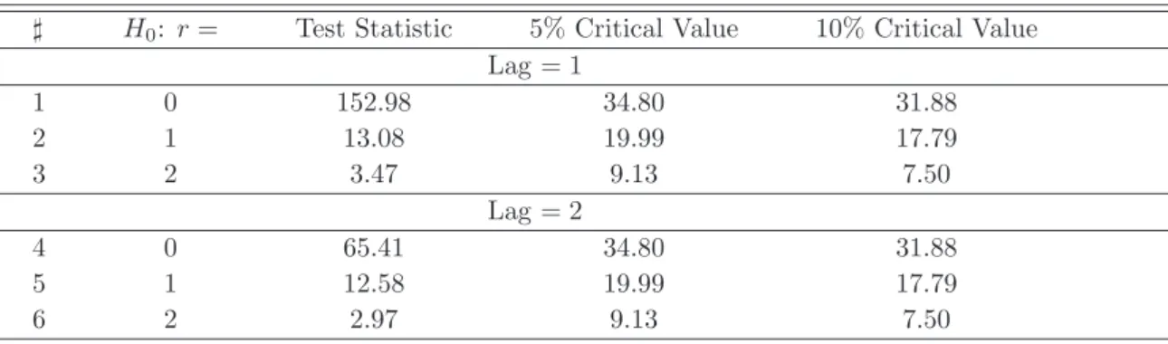
The cointegration relation among nondurables consumption, household net worth, and labor income is the fundament of the theory of the consumption-wealth ratio. Thus, this relation is investigated first. Table (1) reports results of the augmented Dickey-Fuller test for unit root. The number of lagged differences is determined according to the Akaike Information Criterion (AIC). As can be seen in Table (1), all the values of the test statistic are greater than the corresponding 5% and 10% critical values. The null hypothesis of unit root is not rejected for all three variables. The results of the cointegration test are reported in table (2). The numbers of lags are chosen according to the AIC and Schwarz criterion. As can be seen in Table (2), null hypothesis of rank 0 is rejected for all the cases. By contrast, null hypothesis of rank 1 is accepted for all the cases because of the smaller test statistics compared to both 5% and 10% critical values. Therefore, there is strong evidence in the German quarterly data to support the null hypothesis that nondurables consumption, household net worth, and labor income each contains a unit root and they have a single cointegrating vector. The fundamental assumption of the consumption-wealth ratio is confirmed.
4.2
First Stage: Estimation of Trend Deviation
cay
tImplementing the DLS specification (5) using German data from 1971.1 to 2002.4 generates the following point estimates,
b
cn,t = −3.83
(−45.62)+ 0(28.92.98)at+ 0(3..3098)yt, (11) where Newey-West corrected t-statistics appear in the parentheses below the coeffi-cient estimate. The number of lead/lag lengths of the first differences is 4 according to the AIC. The estimators for the first differences are not listed, because they are not essential for the cay estimation. All the estimates in (11) are significant at the 5% level. However, there might be positive autocorrelation in the residuals, given the value of Durbin-Watson statistic, 0.37. This hints that the DLS specification may not be the best choice for estimating the relation between cointegrated consumption, household net worth, and labor income. Furthermore, it is worth to mention that the sum of the coefficient of household net worth (βa) and the coefficient of income (βy)
is greater than 1. This leads to a λ, which is equal to 1/(βa+βy), being smaller than
1. Thus, according to the equation (3), the total consumption , ct, is smaller than
the nondurables and service, cn,t. This result contradicts the general intuition and
hence does not support the assumption, that the log consumption is just a constant multiple of log nondurables and services.
4.3
Second Stage:
d
cay
tas an indicator of Stock Returns
Based on the estimation results from the DLS specification, corresponding estimated trend deviation caydt can be calculated as cn,t − βbaat −βbyyt. The signalling effect
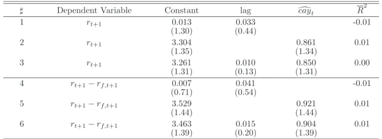
regression. Table (3) presents the results. The real returns and the excess returns are regressed on a constant with either their own lag, or the lagged trend deviation, or both. Neither the estimated trend deviations, dcayt, nor the one lag of dependent variable has significant impact on the real return or the excess return. The statistics of adjusted R2 are around zero.
The signalling effect of dcayt on long-horizon stock returns is investigated with an OLS regression over horizons from 1 quarter to 6 years. Table (4) presents the results of single-equation regressions of either consumption growth or excess returns. Consumption growth is considered here, because the consumption-wealth ratio can signal either the future expected return, or consumption growth, or both, according to equation (4). The dependent variable in Panel A is theH-period consumption growth rate, ∆cn,t+1+· · ·+ ∆cn,t+H. The dependent variable in Panel B is the H-period log
excess returns on the MSCI German stock price index,rt+1−rf,t+1+···+rt+H−rf,t+H.
As can be seen in Panel B, the trend deviation,dcayt, has no significant impact on stock excess returns at any horizon. According to Panel A, the estimated trend deviation,
d
cayt, has significant impact on consumption growth at long-horizons from 2 years to 4 years. These findings from German data are different from the results of Lettau and Ludvigson (2001). They find no impact of cayt on U.S. consumption growth.
Besides, a vector autoregressive (VAR) model is used to investigate the effect of
d
cayt on long-horizon stock returns. Table (5) presents a first-order VAR with two variables: excess returns on the MSCI German index, rt −rf,t and the estimated
trend deviation, dcayt. As can be seen in Row 1, the coefficient of dcayt on excess returns is not significant.
Therefore, no matter which method is used in the second stage, the estimated deviation dcayt has no significant impact on the German stock returns.
5
Performance of
cay
with VECMs
In this section, VECMs are adopted to analyze the signalling effect of cay on stock returns in both German and U.S. data sets. Quarterly U.S. data from 1952.4 to 1998.3 are taken from Lettau and Ludvigson (2001). A single cointegrating vector is included, according to the Johansen trance test of cointegration for German data in table (2) and the analysis for U.S. data in Lettau and Ludvigson (2001). A constant is included in the equation. Based on the AIC, the Schwarz criterion, and the Portmanteau test of the error terms, order 2 is chosen for German data and order 3 for U.S. data.
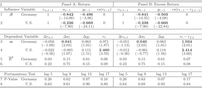
Table (6) shows the estimation results of the long-term parameters, α and β, in the basic VECM. As can be seen in row 1 and 2, all the estimators of the cointegrating vectors (β) are significant at the 5% level. Household net worth has a much higher weight in the common trend of consumption, wealth, and income for Germany than for the U.S.. Compared with the DLS estimation results in equation (11), Johansen approach provides a smaller coefficient on asset wealth and a greater coefficient on income. Besides, according to the last two rows in table (6), all the p-values of the portmanteau test are greater than 5%. There are no significant autocorrelations in the estimated residuals.
Based on the results of the VECM, the Conditional VECM can be conducted. In the VECM for Germany, consumption growth, ∆cn,t, and income growth, ∆yt,
get the most insignificant influence from trend deviations. The absolute values of
t-statistics for the corresponding estimates in α are smaller or equal to 1.1 in table (6). Thus, consumption and income are taken as exogenous for German data in the Conditional VECM. Based on the same argument, consumption and wealth are treated as exogenous for U.S. data. The results from the Conditional VECM are shown in table (7). Compared with the results of the VECM in table (6), the t-statistics of the coefficients in the long-term vectors, α and β, have increased.
Finally, table (8) provides the estimation results of the Conditional-Subset VECM. The estimators ofβ are taken from the results of the Conditional VECM in table (7). The Conditional-Subset VECM provides the highest t-statistics of the remaining α
parameters among all the analysis of VECMs. The estimated consumption-wealth ratio has a significant impact on the wealth growth and (excess) returns in German data, and a significant impact on the income growth and (excess) returns in U.S. data. The signalling effect of the estimated trend deviations on returns is about two times greater in the U.S. than in Germany. The estimated coefficient on the trend deviation for U.S. real returns (excess returns) is about 2.440 (2.293) and for German real returns (excess returns) is about 1.058 (1.140). The results for the U.S. are similar to those via the two-stage method in Lettau and Ludvigson (2001). Their estimated coefficient ondcay for real returns is around 2.2. Moreover, the adjustedR2
in the regression of stock returns is 0.15 in U.S. data and 0.07 in German data. Stock returns can be better signalled by dcay in the U.S. than in Germany.
6
Conclusions
In this paper, the signalling effect of the fluctuations in the consumption-wealth ratio on German stock returns has been investigated. Two different methods are used: the two-stage method and the VECMs. Using the two-stage method, significant impact of
cay on German stock returns is not found. The DLS technique in the first stage may not be efficient to estimate the coefficients among cointegrated consumption, wealth, and labor income. Compared with the results from the VECM, the DLS approach overestimates the weight of wealth and underestimates the weight of labor income in the regression of consumption. Besides, the two-stage method may lead to the loss of information by having two separated stages to study the performance of cay. When the VECMs are used, there is evidence to support the view that cay signals real stock returns and excess returns in both German and U.S. data sets significantly. The Conditional-Subset VECM provides the most precise results. The effect of cay
on stock returns is two times greater in U.S. data than in German data. A Model with the consumption-wealth ratio might be more suitable for U.S. stock returns than for German stock returns. Besides, the results for U.S. are similar to those via the two-stage method by Lettau and Ludvigson.
In addition, two new evidences have been found in the analysis. First, with the Conditional-Subset VECM, cay has impact not only on stock returns, but also on
wealth growth in Germany and income growth in the U.S.. This evidence cannot be explained by the standard theory of the consumption-wealth ratio. Second, no matter which method is used, the sum of the estimated coefficients on income and wealth for German consumption is greater than 1. This result is against the assumption made by Lettau and Ludvigson (2001) that the log consumption is just a constant multiple of log nondurables and services.
References
Campbell, J. Y. & Mankiw, N. G. (1989). Consumption, inocme and interest rate: Reinterpreting the time series evidence, Working Paper 2924, National Bureau of Economic Research.
Cochrane, J. H. (1991). Production-based asset pricing and the link between stock returns and economic fluctuations, The Journal of Finance46: 209–237.
Johansen, S. (1992). Cointegration in partial systems and the efficiency of single-equation analysis, Journal of Econometrics 52: 389–402.
Lettau, M. & Ludvigson, S. (2001). Consumption, aggregate wealth, and expected stock returns, The Journal of Finance 56: 815–849.
L¨utkepohl, H. (1991). Introduction to Multiple Time Series Analysis, Springer Press. Stock, J. H. & Watson, M. W. (1993). A simple estimator of cointegrating vectors in
higher order integrated systems, Econometrica 61: 783–820.
Appendix: Data Construction
The data of stock returns are log real variables from the stock market index. Quar-terly U.S. data from 1952.4 to 1998.3 are taken from Lettau and Ludvigson (2001). U.S. stock returns are returns from the Standard & Poor’s (S&P) Composite Index. The log excess return is obtained by subtracting the log real return on the 30-day Treasury bill (risk-free rate) from the log real return of the index. Quarterly Ger-man data of real stock returns from 1971.1 to 2002.4 is calculated from the Morgan Stanley Capital International (MSCI) German stock price index and MSCI German stock return index. The risk free rate is the German call money rate from the IMF’s International Financial Statistics.
The macroeconomic data such as consumption of nondurables and services, asset holdings, and labor income are quarterly, seasonally adjusted, per capita variables in logarithm. U.S. data are measured in billions of 1992 dollars, taken from Lettau and Ludvigson (2001). German data are measured in billions of 2000 euros1. Data
for consumption of nondurables and services and labor income are obtained from the Federal Statistical Office Germany.
The real obstacle in the data construction is to find suitable German data of asset holdings. Time series of household net worth is generally used as the measure for asset holdings. Because quarterly time series of German household net worth cannot be obtained directly, it has to be constructed based on other available time series. The following four time series are used: annual data of German household net worth from 1991 to 2001 obtained from Datastream, monthly data of deposits of resident individuals at banks (MFIs) in Germany from 1970 to 2003 obtained from the Deutsche Bundesbank2, monthly data of share capital for the whole German market
from 1960 to 2003 obtained from Datastream, annual data of non-financial assets for the whole German economy from 1960 to 1997 obtained from the Federal Statistical Office Germany.
The basic idea of construction is to regress the available short time series of net worth (1991-2001) on the other three variables, and then use the estimated coefficients and the other three variables to construct enough long quarterly time series of net worth. The net worth is regressed on deposits, share, and non-financial assets at a quarterly frequency. If the regression of net worth is at the annual frequency, there are only ten available observations for the net worth. Thus, annual data of net worth and non-financial assets, and monthly data of private deposits and share capital are transformed into quarterly data for the estimation. The annual data are expanded to quarterly data using constant growth rate. The monthly data are transformed to quarterly data using the observations of the last month of the quarter. Besides, Lettau and Ludvigson (2001) use the observation of net worth at the beginning of the period. In order to construct comparable variables, all the transformed quarterly data at the end of this period are treated as the beginning variables at the next period.
Based on the transformed German quarterly data of household net worth, deposits, shares, and non-financial assets from 1992.1 to 2002.1, the following OLS estimates is obtained,
b
wt = 2.44
(3.42)+ 0(4..2613)dt+ 0(3..1840)st+ 0(2..3884)nt, (12) where wt is the household net worth, dt denotes the private deposits, st is the share
capital, and nt presents the non-financial assets. The data used for this estimation
are seasonally adjusted, per capital variables in logarithm, measured in 2000 euros.
t-statistics appear in parentheses below the coefficient estimates. The corresponding
R2 statistic is 0.97. A time trend is not included in the equation because of the
insignificant t-statistic. Figure (1) shows that the fitted household net worth from the regression is very similar to the original series. Based on the estimators in equa-tion (12) and quarterly data of private deposits, shares, and non-financial assets, the quarterly time series of household net worth from 1971.1 to 2002.4 are obtained.
2Private deposits include private transferable deposits, private time deposits, private savings
6 .8 0 6 .8 5 6 .9 0 6 .9 5 7 .0 0 7 .0 5 7 .1 0 9 2 9 3 9 4 9 5 9 6 9 7 9 8 9 9 0 0 0 1 W ealth _ fitted W ealth _ origin al
Figure 1: The original household net worth and the estimated household net worth. The sample period is 1992.1 to 2002.1. The estimated household net worth is calculated by using private deposits, shares, and non-financial assets.
Table 1: Augmented Dickey-Fuller Test for Unit Root
] Variable lag Test Statistic 5% Critical Value 10% Critical Value
1 cn,t 5 -1.18 -2.86 -2.57
2 at 2 -1.62 -2.86 -2.57
3 yt 5 -1.23 -2.86 -2.57
This table reports the augmented Dickey-Fuller test statistics for the variables: consumption of nondurables and services, cn,t, household net worth,at, and labor income yt. For all variables, an
intercept is included.
Table 2: Johansen Trace Test for Cointegration
] H0: r= Test Statistic 5% Critical Value 10% Critical Value
Lag = 1 1 0 152.98 34.80 31.88 2 1 13.08 19.99 17.79 3 2 3.47 9.13 7.50 Lag = 2 4 0 65.41 34.80 31.88 5 1 12.58 19.99 17.79 6 2 2.97 9.13 7.50
This table reports the results of the Johansen trace test for consumption of nondurables and services,
cn,t, household net worth,at, and labor incomeyt. An intercept is included in the test.“Test statistic”
Table 3: Quarterly Regressions of Stock Returns
] Dependent Variable Constant lag dcayt R
2 1 rt+1 0.013 (1.30) (00.033.44) -0.01 2 rt+1 3.304 (1.35) (10.861.34) 0.01 3 rt+1 3.261 (1.31) (00.010.13) (10.850.31) 0.00 4 rt+1−rf,t+1 0.007 (0.71) (00.041.54) -0.01 5 rt+1−rf,t+1 3.529 (1.44) (10.921.44) 0.01 6 rt+1−rf,t+1 3.463 (1.39) (00.015.20) (10.904.39) 0.01 This table reports the estimates from OLS regression of stock returns on lagged trend deviation
d
cayt. The dependent variables are the log real return,rt+1, and the log excess return,rt+1−rf,t+1.
Newey-West correctedt-statistics appear in the parentheses below the coefficient estimate. Table 4: Long-horizon Regressions of Excess Stock Returns
Forecast HorizonH
Regressors 1 2 3 4 8 12 16 24
Panel A: Consumption Growth
d cayt −0.079 (−1.59) [0.01] −0.140 (−1.69) [0.03] −0.166 (−1.46) [0.03] −0.223 (−1.43) [0.04] −0.488 (−2.09) [0.08] −0.772 (−3.13) [0.15] −0.838 (−2.70) [0.14] −0.431 (−0.90) [0.02] Panel B: Excess Stock Returns
d cayt 0.921 (1.44) [0.01] 1.448 (1.06) [0.02] 2.067 (1.15) [0.03] 1.911 (0.93) [0.01] 0.723 (0.27) [−0.01] −2.853 (−1.13) [0.01] −3.827 (−1.14) [0.02] 1.149 (0.29) [−0.01] This table reports the OLS estimates from long-horizon regression of stock excess returns or con-sumption growth on lagged trend deviation caydt. Newey-West correctedt-statistics appear in the
parentheses below the coefficient estimate and adjusted R2 statistics appear in square brackets.
Significant coefficients at the 5% level are highlighted in bold face.
Table 5: Vector Autoregression of Excess Returns
] Dependent Variable constant rt−rf,t caydt R 2
1 rt+1−rf,t+1 3.463
(1.59) (00.015.17) (10..90459) 0.01
2 dcayt+1 −0.587
(−3.24) (10..00811) (170.846.84) 0.73
This table reports the estimates from a first-order vector autoregression (VAR) of the excess returns and the estimated trend deviation term, dcayt. t-statistics appear in the parentheses below the
Table 6: Vector Error Correction Model
] Panel A: Return Panel B: Excess Return
Influence Variable cn,t−1 at−1 yt−1 cs(rt−1) cn,t−1 at−1 yt−1 cs(rt−1−rf,t−1) 1 β Germany 1 −0.842 (−14.08) (−−03.496.96) 0 1 (−−014.841.35) −(−04.503.08) 0 2 U.S. 1 −0.226 (−7.80) (−−024.669.11) 0 1 (−−07.238.90) (−−022.660.84) 0 Dependent Variable ∆cn,t ∆at ∆yt rt ∆cn,t ∆at ∆yt rt−rf,t 3 α Germany −0.050 (−1.09) 0(2.041.03) (10..06301) (10.971.87) (−−01..05113) 0(2.040.03) (10.063.01) 1(2.034.01) 4 U.S. −0.022 (−0.56) −(10..07)085 (10..11551) 2(3.460.59) (−−00..01230) (−−00..06177) (10.118.56) 2(3.414.60) 5 R2 Germany 0.03 0.15 0.01 0.06 0.03 0.15 0.01 0.07 6 U.S. 0.22 0.75 0.15 0.09 0.23 0.75 0.15 0.08
Portmanteau Test lag 5 lag 9 lag 13 lag 17 lag 5 lag 9 lag 13 lag 17
7 P-Value Germany 0.26 0.62 0.07 0.16 0.26 0.63 0.07 0.17
8 U.S. 0.63 9.61 0.90 0.80 0.64 0.69 0.93 0.84
This table reports the estimates from the vector error correction model of consumption, wealth, income, and stock returns. Johansen approach is used. The dependent variables in panel A are difference in consumption of nondurables and services (∆cn,t), difference in wealth (∆at), difference in income (∆yt), and log real return (rt), while in panel
B the return variable is log excess return (rt−rf,t). csdenotes the cumulative sum of the corresponding variable.
t-statistics appear in the parentheses below the coefficient estimate. A constant is included. Significant coefficients at the 5% level are highlighted in bold face.
Table 7: Conditional Vector Error Correction Model
] Panel A: Return Panel B: Excess Return
Influence Variable cn,t−1 at−1 yt−1 cs(rt−1) cn,t−1 at−1 yt−1 cs(rt−1−rf,t−1) 1 β Germany 1 −0.832 (−46.10) (−−023.550.86) 0 1 (−−026.831.98) (−−024.557.14) 0 2 U.S. 1 −0.236 (−14.35) (−−041.658.25) 0 1 (−−014.244.57) (−−036.653.97) 0 Dependent Variable ∆cn,t ∆at ∆yt rt ∆cn,t ∆at ∆yt rt−rf,t 3 α Germany 0.043 (2.52) (10.870.90) (20.043.53) 0(2.940.08) 4 U.S. 0.135 (2.02) 2(4.676.09) (10.128.95) 2(4.554.01) 5 R2 Germany 0.17 0.04 0.17 0.05 6 U.S. 0.32 0.14 0.32 0.13
Portmanteau Test lag 5 lag 5 lag 13 lag 17 lag 5 lag 9 lag 13 lag 17
7 P-Value Germany 0.59 0.96 0.68 0.66 0.60 0.97 0.66 0.66
8 U.S. 0.90 0.93 0.99 0.96 0.88 0.91 0.99 0.95
This table reports the estimates from the conditional vector error correction model of consumption, wealth, income, and returns. Johansen approach is used. The dependent variables in panel A are difference in consumption of nondurables and services(∆cn,t), difference in wealth (∆at), difference in income (∆yt), and log real return (rt), while in panel
B the return variable is log excess return (rt−rf,t). csdenotes the cumulative sum of the corresponding variable.
t-statistics appear in the parentheses below the coefficient estimate. A constant is included. Significant coefficients at the 5% level are highlighted in bold face.
Table 8: Conditional-Subset Vector Error Correction Model
] Panel A: Return Panel B: Excess Return
Dependent Variable ∆cn,t ∆at ∆yt rt ∆cn,t ∆at ∆yt rt−rf,t 1 α Germany 0.052 (3.37) 1(2.058.20) (30.052.37) 1(2.140.37) 2 U.S. 0.171 (2.93) 2(4.440.53) 0(2.166.85) 2(4.293.52) 3 R2 Germany 0.20 0.07 0.20 0.07 4 U.S. 0.34 0.15 0.34 0.15
Portmanteau Test lag 5 lag 5 lag 13 lag 17 lag 5 lag 9 lag 13 lag 17
5 P-Value Germany 0.37 0.86 0.56 0.66 0.36 0.86 0.54 0.66
6 U.S. 0.54 0.82 0.98 0.88 0.86 0.91 0.99 0.95
This table reports the estimates from the conditional-subset vector error correction model of consumption, wealth, income, and returns. The dependent variables in panel A are difference in consumption of nondurables and services (∆cn,t), difference in wealth (∆at), difference in income (∆yt), and log real return (rt), while in panel B the return
variable is log excess return (rt−rf,t). t-statistics appear in the parentheses below the coefficient estimate. A constant