Machine Learning with H2o and R: A Big Data problem

(1)

Grau en enginyeria informàtica

Machine Learning with H2o and R: A Big Data problem.

Memory

Ricard Gardella Garcia

TUTOR: Dr. Xavier Font Aragonès

Spring 2017

(2)

(3)

Dedicated to:

My grandfather, Pere Gardella, the only engineer of the family, an inspiration and role model to me.

(4)

(5)

Thanks to:

(6)

(7)

Resum

Big data i "machine learning" són peces claus en moltes empreses, governs i laboratoris d'investigació. Aquest projecte desenvolupa una solució, partint amb un número de dades extraordinàriament gran, per finalment, reduir-los per poder tractar-los i desenvolupar estadística descriptiva i models de "machine learning" i comparar-los per veure quin soluciona el problema d'una manera més eficient.

Resumen

Big data y “machine learning” son piezas claves en muchas empresas, gobiernos y laboratorios de investigación. Este proyecto desarrolla una solución, partiendo con un número de datos extraordinariamente grande, para finalmente, reducirlos para poder tratarlos y desarrollar estadística descriptiva y modelos de “machine learning” y compararlos para ver cuál soluciona el problema de una manera más eficiente.

Abstract

Big data and "machine learning" are key pieces in many companies, governments and research laboratories. This project develops a solution, starting with an extremely large amount of data, to finally reduce it to be able to treat them, develop descriptive statistics and machine learning models, and compare them to see which solves the problem in a more efficient way.

(8)

(9)

I

Index.

Figure Index. ... III

Table Index. ... VII

Term Index. ... IX

1. Introduction. ... 1

2. Theoretical Framework. ... 3

2.1. Big Data era. ... 3

2.2. Machine Learning. ... 5

2.2.1. Classification. ... 5

2.2.2. Regression. ... 6

2.2.3. Clustering. ... 7

2.2.4. Machine Learning performance. ... 8

2.3. Deep Learning. ... 8

2.3.2. Architecture. ... 9

2.3.4. The overfitting problem ... 9

2.3.5. Deep Learning and Big Data. ... 10

2.3.6. Software implementations. ... 10

2.4. Why using R and H2o. ... 11

2.4.1. What is R? ... 11

2.4.2. Why using R? ... 12

2.4.3. What is H2o? ... 12

2.4.2. Why using H2o? ... 13

3. Objective. ... 15

3.1. Main objectives. ... 15 3.2. Secondary objectives ... 15

4. Referent analysis ... 17

5. Methodology ... 19

6. Development. ... 21

6.1. Data used. ... 21

6.1.1. Columns of the files year.csv ... 21

(10)

II

6.2. Data management. ... 22

6.3. Descriptive statistics and descriptive analysis ... 24

6.4. Machine Learning. ... 29

6.4.1. H2o starting and data preparation. ... 29

6.4.2. Deep Learning parameters. ... 31

6.4.3. First Deep Learning model, ... 31

6.4.4. Tuned Deep Learning model, ... 35

6.4.5. Faster Deep Learning model. ... 38

6.4.6. GLM. ... 41

6.4.7. Same models, but with less parameters. ... 44

6.4.8. Development conclusions. ... 45

6.4.9. Problems in the developing. ... 46

6.4.10. Libraries used. ... 47

7. Conclusion. ... 49

(11)

III

Figure Index.

Fig. 2.1. Clustering example in R 7

Fig. 2.2. Neuron network architecture. 8

Fig. 2.3. Overfitting problem. 10

Fig. 2.2. H2o official webpage. 13

Fig. 5.1. Merge holidays flights in one data set. 23

Fig. 5.2. Creation of new columns. 23

Fig. 5.3. Insert of states into dataHolidays. 23

Fig. 5.4 . Arrival Delay histogram. 24

Fig. 5.5 . Departure Delay histogram. 24

Fig. 5.6 . Logarithmic Arrival Delay histogram. 25

Fig. 5.7 . Logarithmic Departure Delay histogram. 25

Fig. 5.8 . Relation between arrival delay and departure delay. 26

Fig. 5.9 . Relation between ArrDelay and OriginState 26

Fig. 5.10 . Relation between DepDelay and OriginState. 27

Fig. 5.11. Airports map. 28

Fig. 5.12. Airports map interaction. 28

Fig. 5.13. Airports map code. 29

Fig. 5.14. Installation H2o in RStudio. 29

(12)

IV

Fig. 5.16. Connection details. 30

Fig. 5.17. Data splits. 30

Fig. 5.18. Variable specification. 31

Fig. 5.19. Standard Deep Learning. 32

Fig. 5.20. Summary model1. 33

Fig. 5.21. Model1 Performance. 34

Fig. 5.22. Mean model one. 34

Fig. 5.23. Error model one. 35

Fig. 5.24. Model1 predicted vs. real arrival delay. 35

Fig. 5.25. Tuned deep learning model.. 36

Fig. 5.26. Summary tuned model. 36

Fig. 5.27. Performance tuned model. 37

Fig. 5.28. Mean tuned model. 37

Fig. 5.29. Error tuned model. 37

Fig. 5.30. Predicted delay vs. real delay tuned model. 38

Fig. 5.31. Faster Model. 38

Fig. 5.32. Summary faster Deep learning model. 39

Fig. 5.33. Performance faster model. 40

Fig. 5.34. Mean faster model. 40

Fig. 5.35. Error faster model. 40

(13)

V

Fig. 5.37. GLM model. 41

Fig. 5.38. Summary of GLM model. 42

Fig. 5.39. Performance GLM model. 43

Fig. 5.40. Mean GLM model. 43

Fig. 5.41. Error GLM model. 43

Fig. 5.42. Predicted delay vs. real delay GLM model. 44

Fig. 5.43. Less parameters variables. 44

Fig. 5.44. Performance tuned model with less variables. 45

Fig. 5.45. Mean tuned model with less variables. 45

(14)

(15)

VII

Table Index.

(16)

(17)

IX

Term Index.

TFG Final Degree Project MSE Mean Square Error MAE Mean Absolute Error GLM Generalized Linear Model

(18)

(19)

Introduction 1

1. Introduction.

Big data and machine learning are key pieces of many corporations, governments and research labs.

The objective of this TFG is to understand and analyse how machine learning works, using different algorithms, comprehend and analyse the data with descriptive statistics and understand the magnitude of a big data problematic.

Using R, R Studio IDE and H2o, this project studies the behaviour of different machine learning models using a large amount of data that previously have been processed and studied in order to solve a problematic.

(20)

(21)

Theoretical Framework 3

2. Theoretical Framework.

2.1. Big Data era.

Companies are starting to realize the importance of using more data in order to support decision for their strategies. This was said on the data base system journal[1] and it is a good definition of what big data is nowadays.

Many devices produce data and not just mobile phones and computers. With the appearance of the Internet of Things, even more devices produce data, such as, cars, TV's, etc. And of course, not only the devices that make our lives easier produce data, high tech lab devices also produces tons of data that helps later on in the research.

That's why, new systems of data processing are needed, because it is impossible for the traditional data processing software to process that amount of data. There are a lot of tools to manage Big Data, such as Hadoop, NoSql, Cassandra, etc.

The Big Data tools, manage one or more than one type of big data

• Structurated data: This data is defined in length and in format, for example

excel workbook or a data base.

• Non structurated data: Non format data, like an email.

• Semistructurated data: Data that contains marks, like HTML or XML.

We are creating data constantly. Depending of the origin of the data we can classify the data in different groups:

• Generated by the people: All the data that, we the people, generates everyday, for example, sending a WhatsApp message or updating our Facebook profile.

• Data transactions: Transactions between two accounts, for example, two bank accounts.

• E-Marketing: In the web 2.0, the tracking tools generates a good amount of data, such as the heat map, that tracks all the mouse movements in the website.

(22)

4 Machine Learning with H2o and R: A Big Data problem. - Memory

• Machine to Machine (M2M): Technologies sharing data, for example, temperature

sensors, sound sensors, etc.

• Biometrics: Data that comes from security and intelligence services. Data such as digital prints, ADN chains, etc.

Big data have many applications, nowadays; a lot of industries and entities use Big data. The business of Big Data worth more than 100$ million and is growing 10% per year, double than all the software industry combined.

These are the industries were Big Data is used more:

• Government: The governments are adopting the usage of big data for the

improvement of productivity, innovation, etc.

• International development: Research on the effective usage of information and

communication technologies for development suggests that Big data technology can make some contributions. Advances in Big Data analysis offer cost-effective opportunities to improve decision-making critical decisions, such as crime, healthcare, etc. Additionally, the user-generated data offers new opportunities

• Manufacturing: Improvements in the product quality provide the greatest

benefit of big data for manufacturing. Big data provides an infrastructure for transparency in manufacturing industry, which is the ability to unravel uncertainties such as inconsistent component performance and availability.

• Healthcare: Big data in healthcare has helped to provide personalized analytic,

predict clinical risks, predict analytics and even waste and care reduction.

• Education: Universities make usage of Big Data for research and for educational

purposes.

• Media: Usage of Big data in this field is different from the other ones. The

industry is moving away from the traditional approach, and now, uses Big Data for targeting consumers, data-journalism and Data-capture.

• IoT (Internet of Things): Big Data and IoT work together. The Big Data

software consumes all the data generated by the IoT devices.

• Technology: A lot of tech companies use Big Data, for example: Amazon, eBay,

Facebook, Google, etc.

(23)

the tests. 150 million sensors delivering data 40 million times per second, to be clear, the Hadron generates 500 quintillion bytes per day, 200 times more than all the other sources of the world combined.

We can conclude that big data is used in a lot of environments and that it is an angular piece of a lot of areas and it will even more important in the years to come, because, every day more data is generated in these areas.

2.2. Machine Learning.

Machine learning is a subfield of computer science, that can be defined with this statement “Gives computers the ability to learn without being explicitly programmed” according to Arthur Samuel, the computer scientist who coined the term.

Machine learning is related, and sometimes overlapped with computer statistics, because machine learning focuses on prediction making, also it is strong related with mathematical optimization.

The machine learning can be classified in three main types depending on the signal or the feedback of the system, these are:

• Supervised learning: Analyse training data and produces inferred functions, which can be used to analyse new data. Some applications of supervised learning are: Handwriting recognition, spam detection, pattern recognition, etc.

• Unsupervised learning: The observations given are not label, that’s because there is no estimation of accuracy of the output structure, this is the main difference between the other two categories. Some applications of unsupervised learning are: Sentence segmentation, Machine translation, etc.

• Reinforced learning: The environment where the program interacts is dynamic, so, the behaviour of the program changes depending of the context, to maximize the performance. Some applications of the reinforced learning are: Manufacturing, Finance sector, Inventory management, etc.

2.2.1. Classification.

The classification method tries to identify the belonging to a group using labels. An example could be spam detection, using labels, the software decides that that mail

(24)

belongs to the “spam” group. The classification method is divided in two different types, those who use only two labels, and those who use more than two.

In multi class, an object can be assigned to more than one class. The Bayesian procedures are inside this type of machine learning

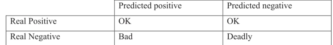
The confusion matrix is also a key piece in the classification methods. The confusion matrix, also called error matrix, normally used in supervised learning, is a table with the errors and the strikes of a prediction. The table 2.1 shows the aspect of a confusion table. In the table 2.1 the problematic analysed is if a patient has or do not have cancer. In this case, a false positive is better than a false negative, for obvious reasons. The confusion matrix always have to be interpreted and the model upgraded according to the problematic.

Predicted positive Predicted negative

Real Positive OK OK

Real Negative Bad Deadly

Table 2.1. Example of cancer confusion matrix.

2.2.2. Regression.

The regression mode main objective is to predict a value of a continuous variable. In other words, we are constantly predicting the value of the same variable in base of his environment.

• Lineal regression:

Used to compute the relation between a dependent variable Y, independent variables Xi, and a random value ε.

This model can be explained as the equation 2.1 shows.

𝑌𝑡 =𝛽0+𝛽1𝑋1+𝛽2𝑋2+...+𝜀 (2.1) • General Lineal Mode:

This model can be explained as the equation 2.2 shows:

(25)

Where Y is the matrix of various measurements of the same variable, X is a matrix of design; B is a matrix of values that are usually estimated and U is the matrix containing error.

• Generalized Linear models:

Generalized Linear Models (GLM’s) are framework for modelling a response variable Y that is bounded or discrete. Every type of GLM serves a different porpoise.

Some examples of common GLM’s are: • Poisson regression

• Logistic regression • Gaussian regression

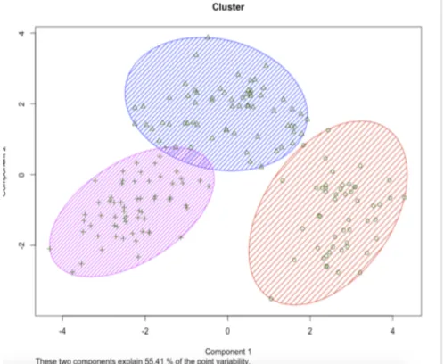
2.2.3. Clustering.

Clustering is the technique of grouping a set of objects in different groups, called clusters, in the way that the objects of the same cluster are more similar than the other objects of other clusters. Is the main technique used in data mining and used in statistical data analysis. The figure 2.1. shows the result of a clustering method in R

(26)

2.2.4. Machine Learning performance.

There are many ways to compute the performance of a Machine Learning model. Normally, the most useful way to do it is with the interpretation of the model itself, to see if the predictions made on the model solves the problematic or not.

But, there are statistics that can give valuable information about the machine learning models.

• MSE: Mean Squared Error, measures the average of the squares of the errors, it is a risk function and a quality measure of an estimator, the lower the MSE, better the estimator. It is important to have in mind that depending of the used data, it is impossible to get a small value, for example, if the data is very scattered to the regression line. The MSE model can be explained with the equation 2.3.

(2.3) • MAE: Mean Absolute Error, is the difference between two continuous variables, assuming that both variables are observations of the same problematic. MAE can be explained as the equation 2.4 shows.

(2.4)

2.3. Deep Learning.

Deep learning is a technique of data extraction and transformation, which can be supervised or non-supervised. Those algorithms work with layers, simulating the brain using neurons. All the layers of the deep learning represent the neurons of the brain. Those terms were introduced by by Kunihiko Fukushima in 1980.

There are different ways to implement Deep Learning, but as said, the most common way to do it is to use neuron networks.

A neuron network is a mathematic tool that simulates the brain and the neurons, in another words; a neuron network operates some mathematic operation over a set of numbers and gives a set of different numbers as result.

(27)

2.3.2. Architecture.

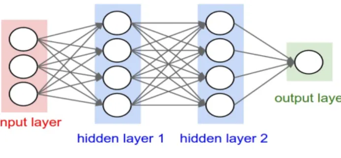
The figure 2.2 is a good representation of what the architecture of a neuron network is:

Figure 2.2. Neuron network architecture

As seen in the image, there is an input layer, two hidden layers and an output layer. • Input layer: is the layer that receives all the input numbers

• Output layer: Is the layer that receives the output once the network had processed all the input values. The output is the result and a set of numbers

• Hidden layers: The hidden layers contain hidden calculus of the network.

As seen before, the model is similar to a black box, what happens in the hidden layers can’t be seen.

It is common that all the neurons have a connection with all the neurons in the next level and those connections have a preference value. The principal operation of the networks is to multiply the values with the preference value of each neuron connection preference value. Then, each neuron of the next layer receives numbers of several connections and the neuron adds them all.

The neuron network, as a machine learning model, can learn supervised, unsupervised or reinforced

2.3.4. The overfitting problem

When there is a model that performs very good with the training data but in the reality it performs really poorly, the problem encountered is called overfitting, that happens when the model have too many parameter and very few data to be trained, the figure 2.3 shows what an overfitting problem will look like [3].

(28)

Figure 2.3. Overfitting problem.

2.3.5. Deep Learning and Big Data.

Big Data Analytics and Deep Learning are two high-focus of data science. Big Data has become important, as many organizations both public and private have been collecting massive amounts of data.

A key benefit of Deep Learning is the analysis and learning of massive amounts of unsupervised data, making it a valuable tool for Big Data Analytics where raw data is largely unlabeled and un-categorized that’s why, Deep Learning can be utilized for addressing some important problems in Big Data Analytics, including extracting complex patterns from massive volumes of data, semantic indexing, data tagging, fast information retrieval, and simplifying discriminative tasks.

But also, Deep Learning research that need further exploration to incorporate specific challenges introduced by Big Data Analytics, including streaming data, high-dimensional data, scalability of models, and distributed computing.

2.3.6. Software implementations.

Tensor Flow:

Tensor flow is an open source library of machine learning created by Google to satisfy their needs of systems capable of building and training neuronal networks. Currently is

(29)

used in both Google research and Google products.

Tensor flow originally was created under the name of Google Brain for internal Google usage. Now, it is under the Apache open source license. As an open source library, it is possible to download it, work with it or even, modify it, here is the link of the official website where the library can be downloaded: https://www.tensorflow.org

H2o:

H2o is an open source software for Big Data analysis, created by the H2o.ai company. H2o also allows users to use their machine learning capabilities, deep learning included. H2o software can be used with R, Python, Java and other environments; it is currently used to analyse large amounts of data in Apache Hadoop as well in operating systems, such as Windows, Linux or macOS.

Azure:

Microsoft has also developed is own machine learning platform and it has been included to the Azure platform. It includes thousand of packages and allows users to work with R or Python but following the structure of Azure Machine Learning.

One of the greatest advantages of Azure is its facility in the deployment of solutions in the Cloud.

Amazon:

Amazon is a company very known by the good usage of the data.

Amazon Machine Learning allows users to make predictions with the tested technology of amazon that their own data scientist have been using for years. It is a pay service, but it is scalable, that means that more resources use the application, more you pay.

2.4. Why using R and H2o.

2.4.1. What is R?

R is a language and environment for statistical computing and graphics. It is a GNU project which is similar to the S language and environment. R can be considered as a

(30)

different implementation of S. There are some important differences, but much code written for S runs unaltered under R.

R provides a wide variety of statistical and graphical techniques, and is highly extensible.

One of R’s strengths is the ease with which well-designed publication-quality plots can be produced, including mathematical symbols and formulae where needed.

R is available as Free Software.

These are the main characteristics of R:

• An effective data handling and storage facility.

• A suite of operators for calculations on arrays, in particular matrices. • A large collection of tools for data analysis and descriptive statistics.

• Graphical facilities for data analysis and display either on-screen or on hand copy. • A well-developed, simple and effective programming language, which includes

conditionals, loops, user-defined recursive functions and input and output facilities.

• A wide community and a lot of libraries for expanding the language.

2.4.2. Why using R?

As said before, R is a language for statistical computing but it is also compatible with H2o. H2o is of mandatory usage in this project. The other options are C# and Java. I chose R over C# and Java, because R is more appropriate for statistical problems and also as a personal choice.

2.4.3. What is H2o?

H2o is an open source software for Big Data analysis, created by the H2o.ai company. H2o also allows users to use their machine learning capabilities, deep learning included. H2o software can be used with R, Python, Java and other environments.

It is currently used to analyse large amounts of data in Apache Hadoop as well in operating systems, such as Windows, Linux or macOS. The creators of H2o are teachers and students of Stanford University. The figure 2.3 shows the official web page of H2o, which is: https://www.h2o.ai.

(31)

Figure 2.3. H2o official webpage.

2.4.2. Why using H2o?

As said before, H2o is of mandatory usage in this project. Also, H2o, is an open source Big data analysis and that allows to develop de project with any external monetary cost.

(32)

(33)

Objective 15

3. Objective.

The objective of this practical deployment is to analyse and compute via descriptive statistics and machine learning, the delay in flights on the holidays days and the surrounding days in the USA. The holidays are the days with more air traffic in all over the country and it is then where the problems can appear, because, There is much more air traffic. It is not common, if not impossible, that an airport works well on vacation

and bad the rest of the year. The holidays have more air traffic and the consequence of

more air traffic, is more delay in the flights.

3.1. Main objectives.

• Following a data science and Big Data process (Collect, prepare, represent, model, reason and visualize).

• Learning to use a set machine learning tools.

• Learning to use descriptive analytics on a large data set. • Creation of machine learning models.

• Compare and analyse the machine learning models.

3.2. Secondary objectives

• Learning in more depth the language R.

• Learning in more depth the environment R Studio IDE.

• Search, install and try a lot of different libraries for different objectives. • Dealing with a Big Data problem.

(34)

(35)

Referent analysis 17

4. Referent analysis

H2o is a machine learning platform that is popular nowadays, but is rather new. The fields of Machine Learning and Big Data are rather new too.

It was impossible to find any referent that creates machine learning models and compare them to see which is better.

The air traffic companies probably have machine learning tools but with the objective to predict real-time delays, not just compare machine learning models.

(36)

(37)

Methodology 19

5. Methodology

In order to develop the TFG in a correct way, I followed these steps, that are usually found in Big Data and Machine Learning problems. The steps followed are listed below: 1. Understand the data and the structure of the data before starting to work with it. 2. Clean the data from non valid arguments such a empty values on fields

3. Descriptive analytics once the data has been cleaned and processed. 4. Starting of the H2o software

(38)

(39)

Development 21

6. Development.

The full code of the development can be found in the appendix one.

6.1. Data used.

In order to solve the problem, we are going to use real data obtained from the American Statistical Association. The data, is about the flights within the USA. The data goes from the 1987 to 2008. Every year is a file .csv (year.csv), that weights approx., 700MB, what makes a total amount of 14700MB. With this amount of data, is correct to talk about a Big data problem.

In order to make the problem efficient and feasible, a cutting of data is needed. Only the years 2006 to 2008 will be taken, which makes a total of 2GB approx., when the data is cropped only with the holidays, the file weights 250MB with 2353000 observations. Another data needed for the project is the data of the airports. The dataset stores all the airports. The file only weights 250KB and it is a .csv.

6.1.1. Columns of the files year.csv

1. Year: 2006-2008

2. Month: 1-12 3. DayofMonth: 1-31

4. DayOfWeek: 1 (Monday) - 7 (Sunday)

5. DepTime: actual departure time (local, hhmm)

6. CRSDepTime: scheduled departure time (local, hhmm) 7. ArrTime: actual arrival time (local, hhmm)

8. CRSArrTime: scheduled arrival time (local, hhmm) 9. UniqueCarrier: unique carrier code

10.FlightNum: flight number 11.TailNum: plane tail number 12.ActualElapsedTime: in minutes 13.CRSElapsedTime: in minutes 14.AirTime. in minutes

(40)

22 Machine Learning with H2o and R: A Big Data problem – Memory

15.ArrDelay: arrival delay, in minutes 16.DepDelay: departure delay, in minutes 17.Origin: origin IATA airport code 18.Dest: destination IATA airport code 19.Distance: in miles

20.TaxiIn: taxi in time, in minutes 21.TaxiOut: taxi out time in minutes 22.Cancelled: was the flight cancelled?

23.CancellationCode: reason for cancellation (A = carrier, B = weather, C = NAS, D = security) 24.Diverted: 1 = yes, 0 = no 25.CarrierDelay: in minutes 26.WeatherDelay: in minutes 27.NASDelay: in minutes 28.SecurityDelay: in minutes 29.LateAircraftDelay: in minutes

6.1.2. Columns of the files airports.csv

1. iata: the international airport abbreviation code 2. name of the airport.

3. city. 4. State. 5. Country.

6. lat: Latitude of the airport. 7. log: Longitude of the airport.

6.2. Data management.

As said before, the main objective of the application is to predict and analyse the delays on the flights within the holidays in the USA. The dates selected as holidays are Christmas from 20 of December to 8 of January, Thanks Giving from 20 of November to 30 of November, Independence Day from 2 of July to 6 of July and Veterans Day from 9 of November to 14 of November.

(41)

Development 23

The files that contain the data, contain all the flights of a year, so, it is necessary, logic and more efficient to crop the data in parts and then merge it together with all the holidays flights from the years 2006 to 2008.

In the figure 5.1 is the code that selects all the holidays flights from the 2006, 2007 and 2008, and returns one file for each year, then, using the rbind function, the years must be merged in one dataset The file created is named dataHolidays. The code is inside a function on a separate file, for code reading porpoises.

Figure 5.1. Merge holidays flights in one data set.

In addition to this, for more complex descriptive analytics, the state origin and the state destination for every flight will be added to the data set. This will be very useful in the future for descriptive analytics. In order to do that, is necessary to create the columns as showed in the figure 5.2. The columns are initialized with the value “a” but any character value can be used.

Figure 5.2. Creation of new columns

After the initialize is done, the code of the figure 5.3 is executed. This code iterates all the airports.csv and checks for every flight his destination and origin IATA code, and adds the correct state for every flight. After several optimizations, this code fills the OriginState and DestinationState in a reasonable time, more or less 5 minutes. It is important to take into account, that filling 2,3 million rows, take some time.

This function is located in a separated file, for code reading porpoises.

(42)

6.3. Descriptive statistics and descriptive analysis

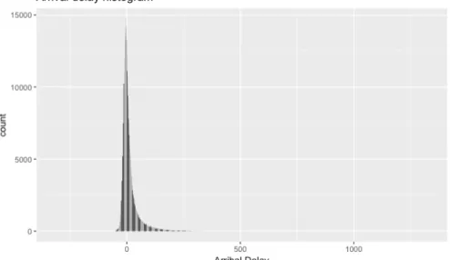
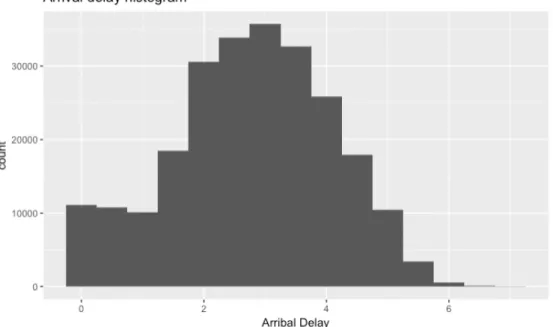
In order to do descriptive analytics in an efficient way, the data must be shortened. The dataHolidays data set has more than two millions rows, so, it is acceptable to cut the data in a smaller part, but enough, for this analysis have been taken 500000 random rows of the dataHolidays data set. The project is focused on the study of the variables Arrival Delay and Departure Delay; the plots of these variables are showed on the figure 5.4 and 5.5

Figure 5.4. Arrival Delay histogram

Figure 5.5. Departure delay histogram

The plots showed before, show the distribution of these variables, but, these distributions are not Gaussian, so, it is interesting to represent the logarithm of these

(43)

Development 25

variables, to see the data in a Gaussian way. The figure 5.6 shows the Arrival Delay logarithmic histogram and the figure 5.7 shows the Departure Delay logarithmic histogram. As said before, these representations are the logarithmic values of the variables Departure Delay and Arrival Delay, not there real values, but these representations can help in the understanding of the data.

Figure 5.6. Logarithmic arrival delay histogram

Figure 5.7. Logarithmic departure delay histogram

The figure 5.8 represents a relation between departure delay and arrival delay. A clear relation is seen in this plot, as higher is the Departure Delay (DepDelay) higher is the Arrival Delay (ArrDelay). This plot confirms what reality shows by itself, that a flight

(44)

with delay on its departure, rarely arrive on time.

Figure 5.8. Relation between arrival delay and departure delay.

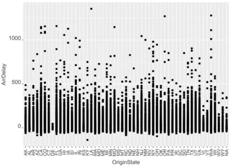
The figure 5.9 shows the relation between the Arrival Delay and the OriginState of the flight. There is no clear relation between arrival delay and state, but is clear that Minnesota, Texas and Wisconsin have more general arrival delay than the other states.

Figure 5.9. Relation between ArrDelay and OriginState

(45)

Development 27

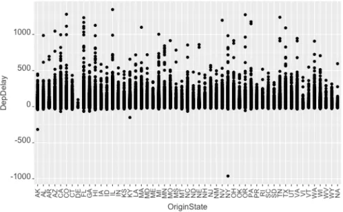
delay. Again, the states with more delay are Texas, Minnesota and Wisconsin. In addition, as proved before, there is a clear relation between departure delay and arrival delay. In the plot a -1000 value can be seen, this point is an extreme value and must be ignored.

Figure 5.10. Relation between DepDelay and OriginState

The figure 5.11 shows a map of all the airports used. In the data there are even more airports, because the military bases, military airports and other installations of the NAVY and the Government of the United States of America are included in the airports.csv. Only the airports recorded in the dataHolidays data set are represented. For the creation of this map the library Leaflet has been used.

The map shows every airport with is total departure and arrival delay and the mean of both variables. There are different representations in color depending of each airport

• Green if the values are correct.

• Orange if the mean of departure delay is bigger than the mean of arrival delay. • Red if the departure delay is bigger than the arrival delay and one of the means is

(46)

Figure 5.11. Airports map

The map is represented in HTML and it is fully interactive, the figure 5.12 shows the interaction with one of the airports and the information showed.

Figure 5.12. Airports map interaction

(47)

Development 29

Figure 5.13. Code for map creation

6.4. Machine Learning.

6.4.1. H2o starting and data preparation.

The H2o software must be installed into our system, if not, it is mandatory to install it. The figure 5.14 shows the code that is necessary to install H2o to R, this code can be found at the official page of H2o.

(48)

After the installation, importation of the library and start H2o is needed. The details of the connection show us the characteristics of the H2o. The figure 5.15 shows the details of the connection.

Figure 5.15. Connection details.

Before starting, in order to work properly with H2o, factoring the character columns is necessary. If this is not done, H2o just discards those columns because the H2o read them as characters, not factors. Once that data is ready, the data must be transformed to the H2o format. This method can take some time if working with a large data set. The figure 5.16 shows the method for transforming a data set to an H2o enviorment variable.

Figure 5.16. H2o environment dataset

The Deep Learning learns about the data that is given to the model, but, to test and validate the model, more data is needed. In order to solve this problem, the data is splited in three parts, one for train the model, other one for validate the model and a last one for test the model, the change of the percentages could cause variations in the final results of the models. The training split of the data should be bigger than the other two in order to obtain efficient models. The figure 5.17 shows the data splits.

Figure 5.17. Data splits.

(49)

Development 31

variable ArrDelay will be the variable studied and the other variables will be the variables used to understand the variable ArrDelay. The figure 5.18 shows how the variables are selected.

Figure 5.18. Variable specification.

6.4.2. Deep Learning parameters.

The Deep Learning method in H2o have a lot of parameters, below, the parameters used in this deployment are explained, the rest of the parameters can be found in the manual [2].

• x: Specifies the vector containing the names of the predictors in the model. No default.

• y: Specifies the name of the response variable in the model. No default.

• training frame: Specifies an H2OFrame object containing the variables in the model. No default.

• model id: (Optional) Specifies the unique ID associated with the model. If a value is not specified, an ID is generated automatically.

• overwrite with best model: Logical. If enabled, overwrites the final model with the best model scored during training. The default is true.

• hidden: Specifies the number and size of each hidden layer in the model. • epochs: Specifies the number of iterations or passes over the training dataset • train samples per iteration: Specifies the number of training samples (globally)

per MapReduce iteration. • rate: Specifies the learning rate .

• input dropout ratio: Specifies the fraction of the features for each training row to omit from training to improve generalization.

• score validation samples: validation error is based on this parameter

6.4.3. First Deep Learning model,

(50)

parameters, without any kind of parameter tuning. These methods take a long time to be executed, as longer data desired to be studied, more time it will take.

Figure 5.19. Standard Deep Learning.

It is highly recommended to save the model if it is desired to work on it later, because, after closing the H2o session, the model is lost.

The figure 5.20 shows the summary of the model 1. The most important information there is the metrics, where the MSE, MAE and Mean residual deviance appear. The scoring history is also important, because, it shows also the time necessary to make the model, 22 minutes and 51 seconds. The time can change depending on the CPU of the computer used.

(51)

Development 33

Figure 5.20. Summary model1

As said before, the data was split in three parts, train, validation and test. When the model is created, is also validated. After the creation, it is interesting to test the model with the test data. The figure 5.21 shows the result of the performance of this model and the code necessary for the obtaining of the performance. The variables showed are the same that the metrics of the summary of model one, showed in figure 5.20, but this data, is contrasted with the test data. The MSE, MAE and Mean residual deviance are the most important information given by this method.

(52)

Figure 5.21. Model1 Performance.

Apart from the performance method that H2o gives, it is interesting to create specific predictions for the problematic.

The predictions are based on the X variable, ArrDelay, which is expressed in minutes. In order to distinct the correct predictions of the incorrect, the formula of the equation 5.1 have been used.

!!!

! ≤0.7 𝑂𝑅 !!!

! ≤ 0.7 (5.1)

The equation 5.1 take the values predicted and the values within the test data set and compare them, if the values of the predicted in relation to the real or the values or the real in relation to the predicted are less different than 70% the prediction is considered correct. It is important to take into account that the values of the delay are positive or negative, for this reason, it is very important to work in absolute values.

A difference of 70% in minutes has been taken, because, it may be an acceptable variation in this context, in other context this variation could be extremely high.

If one of the results is less that 70% of delay error, the prediction is ok, if not, incorrect. The values of correct (1) or incorrect (0) are stored in separated variables.

To see the % of strikes, the mean is calculated. The error can be calculated using 1- the mean.

The figure 5.22 shows the mean and the figure 5.23 shows the error of the model one based on the equation 5.1.

(53)

Development 35

Figure 5.22. Mean model one.

Figure 5.23. Error model one.

In order to understand in a more easy way the model, a plot comparing the predicted and the test data has been made. The figure 5.24 shows the plot comparing the predicted vs the real arrival delay, as seen, the predicted and the arrival. The result is accurate, as it can be seen, the is no big difference between predicted and real, as showed before in figure 5.21, figure 5.23 and figure 5.24.

Figure 5.24. Model1 predicted vs real arrival delay.

6.4.4. Tuned Deep Learning model,

Now, the same operations than before will be made on a tuned deep learning model in order to know if a modification of the parameters of the model increase the performance

(54)

of the model. What it makes this model different is the number of hidden layers, with more layers, there is a more complex and accurate model, also, the score validation sample has been increased for more understanding of the data.

Figure 5.25. Tuned deep learning model.

The figure 5.25 shows the summary of the tuned deep learning model, as can be seen in the figure 5.25, the time is lower than the model1.

(55)

Development 37

The performance of this model is showed in the figure 5.26, with the same information than the performance of the model 1.

Figure 5.27. Performance tuned model.

The same custom prediction has been done in this model; figure 5.27 and 5.28 show the result of those predictions. An increase of the mean is seen in this model, because the increase of hidden layers, validations samples and epochs make this model better.

Figure 5.28. Mean tuned model.

Figure 5.29. Error tuned model.

As done in the model one, the plot is also made for this model, as can be seen, the plot is similar than the one seen in the figure 5.23. The figure 5.29 shows the plot of the tuned model.

(56)

Figure 5.30. Predicted delay vs. real delay tuned model.

6.4.5. Faster Deep Learning model.

The model has been modified again, now, this model, is a lot more faster than the previous one. Lowering the hidden layers, creates an smaller network, more imprecise, but faster. Also, the epochs parameters has been set to one. It can be useful to compare if a more complex and expensive model is really worth. The same operations than before will be performed in order to compare the results. The figure 5.30 shows the configuration of the model:

(57)

Development 39

The figure 5.30 shows the summary of the faster deep learning model with the same information than the summary of the other models. As can be seen in the figure 5.30, the time is low compared to the five to ten minutes that the other models take to be

executed.

Figure 5.32. Summary faster Deep learning model .

(58)

same information than the other performances. The MAE has increased a little bit, for the lack of training of the model.

Figure 5.33. Performance faster Deep learning model .

The same custom prediction has been done for this model. The figure 5.32 shows the mean of this model and the figure 5.33 shows the error.

Figure 5.34. Mean faster Deep learning model .

Figure 5.35. Error faster Deep learning model .

The plot has also been done for this model, the figure 5.34 shows the plot of the faster deep learning model, it is very similar to the other ones due to the similarity on their results.

(59)

Development 41

Figure 5.36. Predicted delay vs. real delay faster model.

6.4.6. GLM.

In order to compare different Machine learning methods for this project, a GLM method has been done on porpoise to compare these models and see if the is a real difference between them and why these differences appear or do not appear.

The figure 5.35 shows the creation of the GLM model, as can be seen, the method is a lot simpler than the deep learning method.

Figure 5.37. GLM model.

The figure 5.36 shows the summary of the GLM model. As can be seen, is different from summaries, because it is a different machine learning method. It is interesting to see the variable importance, where it can bee seen that the most related variable to Arrival Delay is Departure Delay, as I was proved in the descriptive analytics chapter.

(60)

Figure 5.38. Summary of GLM model.

The figure 5.37 shows the performance of the GLM model, the only additional information is the Null Deviance and the Residual Deviance, the null deviance shows how well the response is predicted by the model with nothing but an intercept. The residual deviance shows how well the response is predicted by the model when the predictors are included. Smaller the values, better model, but the value depend on the number of data and predictors of the model.

(61)

Development 43

Figure 5.39. Performance of GLM model.

The figures 5.37 shows the mean and 5.38 show the error based on the equation 5.1. As can bee seen in the figures 5.37 and 5.38, the model is really good, even compared with the deep learning models.

Figure 5.40. Mean of GLM model.

Figure 5.41. Error of GLM model.

Also, as done before with the deep learning, the figure 5.39 shows the plot comparing the predicted and test values.

(62)

Figure 5.42. Predicted delay vs. real delay GLM model.

6.4.7. Same models, but with less parameters.

The same models, with fewer variables on the X and Y have been executed with the variables seen in the figure 5.39, in order to see if there is a difference between executing the models with less variables. These variables have been chosen because there are the variables with more relation to the variables Arrival Delay.

Figure 5.43. Less parameters variables.

(63)

Development 45

performance of the tuned model but with less parameters and the figure 5.41 shows the mean of the tuned model with less parameters based on the equation 5.1 and the figure 5.42 the error based on the equation 5.1. As can be seen, the behaviour of the model is similar, this model have less accuracy than the previous tuned model.

Figure 5.44. Performance of tuned model with less variables

Figure 5.45. Mean of tuned model with less variables

Figure 5.46. Error of tuned model with less variables.

In order to see the variable importance of a deep learning model, the parameter variable importance can be set to true. Now, the model will compute the variable weigh

importance, but only for the first two hidden layers.

6.4.8. Development conclusions.

All the models are similar. The lowest error appears in the tuned deep learning model. This is because that model has more layers and values per iteration. In addition, the GLM model is accurate and is faster than any deep learning model.

The model3 is the fastest deep learning model but the worst model.

The best model depends on the needs of the user. If a fast and precise model is required, the GLM is clearly an option to consider, if accuracy is key, the tuned model is better. With a more accurate study or data cleaning could be possible to archive less error on

(64)

the tuned model, but, a 63% of accuracy is really high, having in mind, that only a variance of 70% of variance of minutes are allowed in order to consider a prediction correct.

In terms of performance, the best model is the model1, without any kind of tuning. It is important to understand that the performance by itself is irrelevant, the important thing is what conclusions can be extracted of the models that are created, and even the model1 have better performance than the tuned model, the tuned model serve our porpoise better. It is important to have in mind that every execution of the model, could give different results on the predictions, not huge variations, but still perceptible, for example, a variation of a 4% in the equation 5.1.

The GLM gets high accuracy because the data is in plain text and structured in a .csv. If the data was images or sounds, the performance of the GLM will decrease dramatically and the deep learning model don’t, because the deep learning also serve those porpoises, as explained in the theory framework.

When it comes to compare the models with more or less variables, is seen that the models with more variables get better results. That’s because a model with more variables have more information about the behaviour of the variable Y. It is important also not to fill the model with unnecessary variables, because it can be contaminated.

6.4.9. Problems in the developing.

There are some problems that have been faced in the developing of this project that are important to mention:

• The data managing have been difficult, because, managing such amount of data have its complexity.

• The machine learning models require that the columns with characters values to be factors, if this is not done, the machine learning model discards the columns. • The merging of the airports data set into the dataHolidays required a lot of

optimization. When working of large amount of data, optimization is key.

• The tuning of a deep learning model requires a lot of caution by the developer, one wrong parameter, could made the whole model collapse.

(65)

Development 47

6.4.10. Libraries used.

There is a list of the libraries used for this project.

• Ggplot2: This library is very popular library, used to represent and make plots, histograms, etc. in a more clear and beautiful way.

• Leaflet: This library is used to create custom maps to represent the information. In the project the library was used to develop the map in the descriptive statistics chapter.

• H2o: This library is the main library of the project. Used to develop all machine learning models.

(66)

(67)

Conclusions 49

7. Conclusion.

Big Data and Machine Learning are key pieces in actual technology, the main objectives of this project was to gather an amount of data, perform descriptive statistics, process it with H2o using machine learning models and compare them.

The conclusion that can be extracted of the project is that machine learning is clearly a central piece of modern technology, as long with the data science field. The predictions made by the models are accurate and with more learning, the more accurate are the models. Another conclusion that can be extracted is that computational power is crucial when working with large data. Optimization has been key for developing this project.

Has been difficult to find and gather this big volume of information as manage and represent the information. In addition, the machine learning modelling has been difficult as the field is really new and the lack of information has been a problem.

Future improvements, like making and application where the user could interact and enter data could be an interesting idea. In addition, developing better models or trying more machine learning methods could improve the results given by this project.

(68)

(69)

8. References.

[1] DataBase Systems Journal vol. III no 4/2012

[2] https://s3.amazonaws.com/h2o-release/h2o/rel-markov/1/docs-website/datascience/deeplearning.html H2o Deep Learning Manual [3]

(70)