Stock return and interest rate risk at Fannie Mae and Freddie Mac

(1)

Stock Return and Interest Rate Risk at

Fannie Mae and Freddie Mac

Frank A. Schmid

the timely payments of principal and interest on these MBS and collect a guarantee fee in return; this is effectively insurance business. The interest rate risk of these MBS resides with the investors that purchase these securities. Second, Fannie Mae and Freddie Mac purchase mortgage-related secu-rities, including their own MBS, and retain these securities; these purchases are mostly financed with debt securities. In this line of business, Fannie Mae and Freddie Mac take on interest rate risk and, unless these assets are securities issued by Ginnie Mae (Government National Mortgage Association), credit risk.1Because the mortgage portfolios of these enterprises are geographically diversified and because, by definition, mortgage loans are collateralized debt, the credit risk is generally held to be small (see the Office of Federal Housing Enterprise Oversight [OFHEO], 2003).2

T

his article examines the sensitivity to

realizations of interest rate risk of the stock returns of Fannie Mae (Federal National Mortgage Association) and Freddie Mac (Federal Home Loan Mortgage Corporation). The study shows that the market value of Fannie Mae’s and Freddie Mac’s equity is vulnerable to increases in short-term interest rates and changes in the term spread (the difference between the long-term and short-term interest rates).

Fannie Mae and Freddie Mac are venues for pursuing the public policy objective of furthering home ownership by improving the availability of mortgage financing for medium- and low-income households. These enterprises are organized as government-sponsored enterprises (GSEs), that is, they are privately operated and funded corpora-tions that are chartered by the federal government. Fannie Mae and Freddie Mac, which are competi-tors, pursue two major lines of business. First, these enterprises purchase mortgage loans, bundle them into mortgage-backed securities (MBS), and sell them to investors. The enterprises guarantee

Fannie Mae and Freddie Mac are government-sponsored enterprises (GSEs) with the stated objective of promoting home ownership by improving the availability of mortgage financing for private house-holds. These enterprises engage in two separate and distinct lines of business: (i) assembling and marketing pools of mortgages on which they guarantee the timely payments of principal and interest and (ii) purchasing mortgage assets for their own portfolio, mostly funded with debt securities. This article examines the sensitivity of the returns on GSEs’ equity shares to realizations of interest rate risk. The study shows that the market value of Fannie Mae’s and Freddie Mac’s equity is vulnerable to increases in short-term interest rates and changes in the term spread (the difference between the long-term and short-term interest rates).

Federal Reserve Bank of St. Louis Review, January/February 2005, 87(1), pp. 35-48.

1

Securities issued by Ginnie Mae are backed by the full faith and credit of the U.S. government.

2

Fannie Mae and Freddie Mac may raise the credit risk of the retained mortgage portfolios by raising the loan-to-value (LTV) ratios of the mortgages they purchase; for mortgages with an LTV greater than 80 percent, these GSEs have to demand credit enhancement (see OFHEO, 2003).

Frank A. Schmid is a senior economist at the National Council on Compensation Insurance, Boca Raton, Florida. The article was written while Schmid was affiliated with the Federal Reserve Bank of St. Louis. Jason Higbee provided research assistance.

(2)

Recent controversies surrounding Fannie Mae and Freddie Mac have concerned the efficacy of subsidizing home ownership through the channel of GSEs and the incentive structure government sponsorship creates at these entities; for an over-view of these controversies, see Frame and Wall (2002a) and Van Order (2000). On one hand, Fannie Mae and Freddie Mac are publicly traded corporations. On the other hand, because these enterprises operate with charters issued by the federal government, they enjoy privileges not available to other companies in the private sector. There is concern that government sponsorship generates extra income to the shareholders by establishing a barrier to entry to the market, pre-venting potential rivals from competing away abnormal profits at Fannie Mae and Freddie Mac (see Hermalin and Jaffee, 1996). Abnormal profits go to the shareholders, the investors that hold the residual income rights. According to a study by the Congressional Budget Office (CBO, 2004), Fannie Mae and Freddie Mac retained about a third of the subsidy that they gathered (see also Passmore, 2003). On the other hand, as pointed out by Frame and White (2004), this surplus is at risk of being eroded through competition from Federal Home Loan Banks and, due to improved risk-based capital requirements laid out in the Basel II regulatory standards, from commercial banks.

In a corporation, the shareholders hold the control rights over the allocation of the assets; this is because bundling control and residual income rights abets the internalization of the consequences of decisionmaking. But these control rights also put the shareholders in a position to behave oppor-tunistically vis-à-vis the debt holders. Remember that the equity of a corporation is a call option on its assets (Merton, 1974). The shareholders may exercise this call by making the promised pay-ments to the debt holders; not exercising this call would entail bankruptcy or, equivalently, the trans-fer of the control rights over the assets to the debt holders. All else being equal, the value of an option increases with the volatility in the value of the underlying asset; here, the underlying asset is the enterprise’s asset portfolio. Put differently, the riskier the firm, the more valuable is the equity; this is why the shareholders have an incentive to

behave opportunistically vis-à-vis the debt holders by taking on more risk than originally stated once the debt holders are invested.3The shareholders can increase the risk of the firm by choosing an asset portfolio with a greater dispersion of pay-offs or by increasing its financial leverage. The Modigliani-Miller theorem implies that financial leverage has no bearing on the value of the firm.4 Remember that the value of the firm is the market value of the assets, which equals the market value of the financial (debt and equity) claims on these assets. Hence, if the shareholders gain from increased leverage, then the debt holders lose. Anticipating the shareholders’ incentives, invest-ors, before underwriting the firm’s debt, insist on collateral or restrict through covenants the share-holders’ choice set.

At Fannie Mae and Freddie Mac, because of government sponsorship, traditional constraints on shareholder risk-taking do not apply. Generally, when investors underwrite corporate debt, they are buying default-free debt—effectively, government debt—and write a put option to the shareholders, giving the shareholders the right to walk away from the firm; the right to walk away is the privi-lege of limited liability (Merton, 1974). At Fannie Mae and Freddie Mac, the debt holders do not seem to perceive themselves as writers of put options; in fact, it appears that the debt holders assume that the government writes these options. This perceived government guarantee explains why the credit quality of Fannie Mae’s and Freddie Mac’s debt is close to default-free. The Federal Deposit Insurance Corporation (FDIC, 2004) states that “if investors were to disregard any implicit guarantee...GSE credit ratings would likely be lowered from the top ratings grades cur-rently issued by major rating agencies. Based on existing studies, we assume that the ratings agen-cies would lower GSE credit ratings within a range of AA to A.”

Schmid

3

Here, risk is total risk, which comprises systematic risk and idio-syncratic risk.

4

If debt is tax-preferred over equity, then financial leverage indeed contributes to the value of the firm. On the other hand, there are bankruptcy costs—the difference between the going-concern value and the liquidation value of the assets accounts for much of these costs. Bankruptcy costs limit the optimal amount of financial leverage.

(3)

The evidence of market discipline provided by Seiler (2003) notwithstanding, there is reason to believe that debt holders impose no effective con-straint on risk-taking at Fannie Mae and Freddie Mac; see, for instance, OFHEO (2003) and FDIC (2004).5Further, the convexity of the enterprises’ excess stock returns in the excess market return, as evidenced in Schmid (2004), suggests that there is a conjectural guarantee for the shareholders as well. The assumed option writer—the government and, ultimately, the taxpayer—limits risk-taking at Fannie Mae and Freddie Mac through a regulator, the OFHEO.6

What follows is an empirical study of the sensitivity of the stock returns of Fannie Mae and Freddie Mac to draws from interest rate risk dis-tributions. The analyzed time period is May 1991 through December 2003; most of this time window overlaps with the existence of the OFHEO, which began operations in 1993. To be parsimonious, I measure realizations of interest rate risk only in two dimensions, which are changes in the level and the slope (or term spread) of the Treasury yield curve.

The next section offers a brief discussion of retained interest rate risk or, synonymously, bal-ance sheet risk at these enterprises. I then describe the data and the variables employed in the empiri-cal analysis, outline the econometric method, and offer the empirical findings and conclusions. There are two appendixes; one contains information on the data sources and definitions of the variables and another describes the econometric approach.

SOURCES OF INTEREST RATE

RISK AT FANNIE MAE AND

FREDDIE MAC

Jaffee (2003) offers a detailed analysis of the interest rate risk that emanates from the debt-financed retained mortgage portfolios of Fannie

Mae and Freddie Mac. Jaffee distinguishes two potential sources of interest rate risk. First, the cash flow of the mortgage assets over time and across interest rate environments may not match with the cash flow of the debt liabilities. Such a mismatch may arise when these GSEs finance their retained mortgage portfolios with short-term debt. Because short rates are lower than long rates most of the time, the difference between the short bor-rowing rate and the long lending rate is a source of income, in particular when the term structure of interest rates is strongly upward sloping. This “carry trade” may cause a duration mismatch between the mortgage portfolio and the debt lia-bilities that finance this portfolio.7If, for instance, the weighted average of the times to maturity of the cash flows of the assets is shorter than the weighted average of the times to maturity of the cash flows of the debt liabilities, then there is a negative duration gap. In such a situation, the liabilities are more sensitive to changes in interest rates than are the assets: When interest rates decline, the assets increase in value less than the liabilities and, hence, the value of the equity declines.

The second potential source of interest rate risk may originate in a mismatch of the prepayment options embedded in the mortgage portfolio and the call options embedded in the debt liabilities that finance this mortgage portfolio—this is the prepayment risk. With their retained mortgage portfolios, Fannie Mae and Freddie Mac have a long position in collateralized debt and a short position in call options on this debt; the house-holds that take out these mortgage loans have a long position in the calls. Writing call options is a source of income: The premium of the call con-tributes to the yield spread between (fixed-rate) mortgages and debt securities of similar duration and default risk. When long rates fall, for instance,

Schmid

5

Seiler (2003) has shown that the share prices and senior-debt yield spreads of Fannie Mae and Freddie Mac indeed respond to news concerning the enterprises’ financial risk and the probability of the government guaranteeing the enterprises’ debt.

6

The OFHEO was established under the Federal Housing Enterprises Financial Safety and Soundness Act of 1992.

7

Duration, also known as Macaulay’s duration, is a weighted average of the times to maturity of a portfolio’s scheduled cash flows. This weighted average is an elasticity that indicates the percentage change in the market value of this portfolio in response to a uniform, 1 percent change in the discount factor for all times to maturity, multiplied by –1. The discount factor for a given cash flow equals 1 + r

t, where rtis the interest rate for the remaining time to maturity

in question, t. The concept of duration assumes that the discount factors (1 + r

(4)

then the value of the call options increases, which subtracts from the market value of the mortgage portfolio. The GSEs can hedge their short position in calls by holding call options on their debt.

From these two sources of risk, Jaffee (2003) derives the perfect balance sheet hedge. Interest rate risk is perfectly hedged if the mortgage port-folio is financed with long-term callable debt such that the cash flow of the mortgage portfolio matches the cash flow of the debt in any interest rate environment, regardless of the amount of mortgage loans that is being prepaid.

Fannie Mae and Freddie Mac do not pursue a perfect balance sheet hedge, in part because these enterprises regard risk-taking as a line of business; as Jaffee (2003) has shown, risk-taking is highly profitable for Fannie Mae and Freddie Mac. Jaffee defines as balance sheet risk the frac-tion of interest rate risk that these GSEs leave unhedged. This author shows that the maturity gap and the short position in call options are signifi-cant sources of income at Fannie Mae and Freddie Mac. Jaffee also offers a detailed analysis of the hedging strategies of Fannie Mae and Freddie Mac. It is ultimately an empirical question of how much interest rate risk these GSEs retain and how much they hedge.

DATA AND DEFINITIONS OF

VARIABLES

I study the sensitivity of the stock returns of Fannie Mae and Freddie Mac to (good or bad) draws of interest rate risk, as perceived by the marginal shareholder; I control for realizations of market risk (or, synonymously, systematic risk); market risk manifests itself in the covariance with the market return of the stock return of the respec-tive enterprise. I allow these stock-return sensitivi-ties to be time-varying.

In keeping with standard practice, I study the logarithmic excess return, that is, the logarithmic return in excess of an investment in the risk-free asset. I choose the Center for Research in Security Prices (CRSP®) value-weighted stock market index as the market portfolio and a eurodollar money market deposit as the risk-free asset. I measure shifts in the level of the yield curve by changes

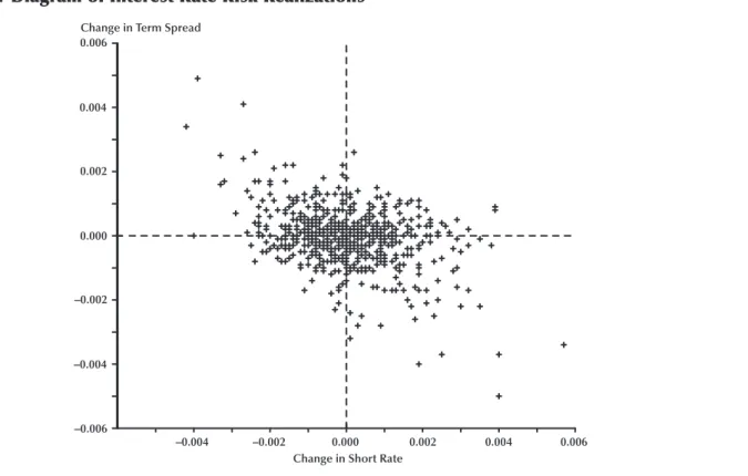
in the 3-month constant-maturity Treasury yield. I gauge changes in the slope (term spread) of the yield curve by changes in the difference between the constant maturity 10-year and 3-month Treasury yields. The variables are on a weekly basis (Friday through Thursday), to avoid potential autocorrelation of returns due to the weekend effect.8The observations run from Friday, May 31, 1991, through Thursday, December 18, 2003. The time period starts when 7-day eurodollar rates became available. For details on the definitions of the variables and the data sources, see Appendix A. Figure 1 offers a scatter diagram of pair-wise observations of changes in the short rate and the term spread. The scatter diagram shows that these two variables are mildly negatively correlated; the correlation coefficient equals –0.43.

EMPIRICAL METHOD AND

RESULTS

In analyzing the sensitivity of the stock returns of Fannie Mae and Freddie Mac to draws from the market risk and interest rate risk distributions, I start out with the nonparametric model

(1) ,

where y

tdenotes the observation of the dependent variable at time t, the vector z_tcomprises the observations of the explanatory variables at time t, and ε_tis an independently and normally distrib-uted error term with mean 0 and constant, finite variance σ2_{. The dependent variable is the 7-day} (Friday through Thursday) logarithmic excess stock return of Fannie Mae or Freddie Mac, respec-tively. The explanatory variables comprise the 7-day logarithmic excess return of the market, the change of the 3-month T-bill yield, the change of the difference between the 10-year T-note and the 3-month T-bill yields during this 7-day period, and a time index. The time index measures the distance of observation t to the first observation

y f

t = (zt)+εt Schmid

8

Abraham and Ikenberry (1994) have documented that when Friday’s stock return is negative, Monday’s return is negative nearly 80 percent of the time, with a mean return of –0.61 percent. Also, when Friday’s return is positive, the subsequent Monday’s mean return is positive, averaging 0.11 percent.

(5)

in the studied time period, measured in number of weeks elapsed, plus 1. The functional form f (•) accommodates an intercept. For details on the econometric method, see Appendix B.

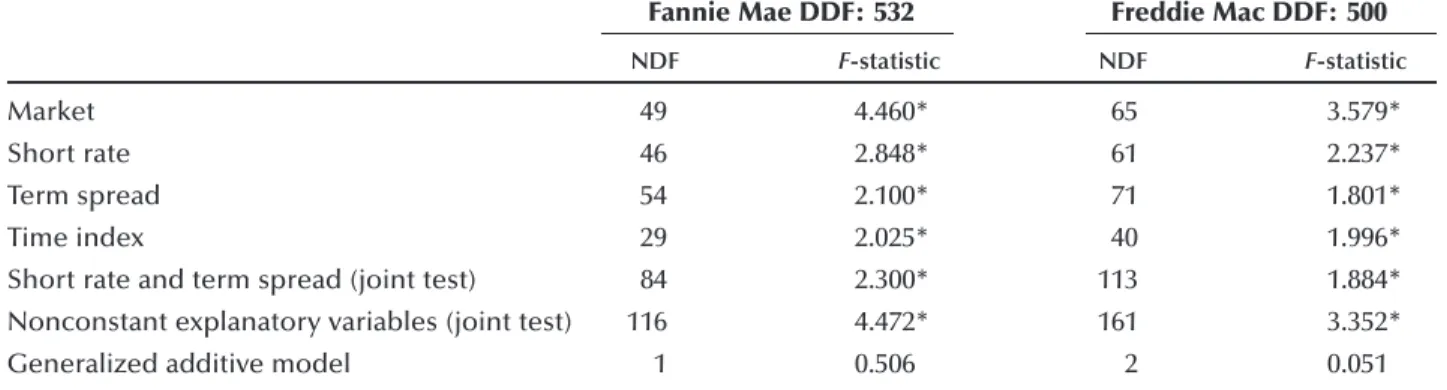
I estimate model (1) using the multivariate smoother LOESS (locally weighted regression) as developed by Cleveland and Devlin (1988) and Cleveland, Devlin, and Grosse (1988); for details on the econometric method, see Appendix B. Table 1 offers an analysis of variance for restric-tions imposed on model (1) (for details on the cal-culation of the test statistic, see Appendix B). The first row (“Market”) shows that the excess stock returns of Fannie Mae and Freddie Mac covary in a statistically significant manner with the market excess return, as expected. Further, these excess stock returns vary in a statistically significant manner with changes in the short rate and the term spread; these variables are statistically significant individually and as a group (joint test). In conclu-sion, I can reject the hypotheses that the stock market perceives Fannie Mae’s and Freddie Mac’s

interest rate risks as perfectly hedged.

Table 1 also offers an analysis of variance for the restriction that the influences on the GSEs’ excess returns of realizations of market risk (on one hand) and interest rate risk (on the other hand) are additive. Imposing such a restriction on model (1) leads to the following generalized additive model:

(2) .

In model (2), the component f₁(•) captures the influence of the log market excess return and the component f₂(•) subsumes the influences of the changes in the short rate and the term spread; both x

tand z˜tinclude the time index, and both com-ponents f₁(•) and f₂(•) provide for an intercept. The test statistic in Table 1 (“Generalized additive model”) does not reject the hypothesis that the influences of market risk and interest rate risk are additive; in what follows, this restriction is imposed. y f x f t = 1( t)+ 2(%zt)+εt Schmid 0.006 0.004 0.002 0.000 –0.002 –0.004 –0.006 –0.004 –0.002 0.000 0.002 0.004 0.006

Change in Term Spread

Change in Short Rate

Figure 1

(6)

Figures 2 (Fannie Mae) and 3 (Freddie Mac) offer quantitative estimates for the sensitivity of the GSEs’ excess returns to draws from the interest rate risk distributions as obtained from the com-ponent f₂(•) of the generalized additive model (2). The estimates shown in these figures are presented in conditioning plots, as introduced by Cleveland and Devlin (1988). Such plots display the esti-mated (partial) impact of a selected explanatory variable with the other explanatory variables pegged at chosen values. Because the intercept is not identified in this type of regression, only changes in the displayed partial impact (rather than the level itself) can be interpreted in an econ-omically meaningful manner. The variable that varies in a given conditioning plot adopts only values observed in the neighborhood of the pegged explanatory variables. Specifically, when I peg a variable to its median negative (positive) value, only observations for which this variable adopts nonpositive (nonnegative) values are included in the conditioning plot. Similarly, when I peg a variable (such as the changes in the short rate or term spread) at zero, only observations for which this variable lies within the closed interval of the median negative and the median positive values are included in the conditioning plot. A similar principle applies to the time index. (For the time index, substitute 25th percentile for median nega-tive value, median for zero, and 75th percentile for median positive value.) At the bottom of each

figure there is a frequency distribution for the variable that varies along the horizontal axis.

The top rows of each panel (A through C) of Figures 2 (Fannie Mae) and 3 (Freddie Mac) dis-play, for three different values of changes in the term spread, the influence of changes in the short rate on the log excess stock returns. In the leftmost plot of the top row, the change of the term spread is pegged at the median negative value; in the center plot, the change is zero; and in the rightmost plot, this variable is kept at the median positive value. The plots show that the log excess returns of Fannie Mae and Freddie Mac are negatively related to changes in the short rate and that this relation is convex. In Panel A, the time index is pegged at its 25th percentile, which is early October 1994; in Panels B and C, the time index is pegged at its median (mid-February 1998) and its 75th percentile (early July 2001), respectively. Late in the studied time period (Panel C), assuming that there is no change to the term spread, a drop in the short rate by 26 basis points (or 0.0026) boosts the excess return of Fannie Mae by 130 basis points; conversely, a rise in the short rate by 30 basis points depresses this return by 231 basis points.9For Freddie Mac, the respective numbers read 105 and 215 basis points.

Schmid

Table 1

Analysis of Variance

Fannie Mae DDF: 532 Freddie Mac DDF: 500

NDF F-statistic NDF F-statistic

Market 49 4.460* 65 3.579*

Short rate 46 2.848* 61 2.237*

Term spread 54 2.100* 71 1.801*

Time index 29 2.025* 40 1.996*

Short rate and term spread (joint test) 84 2.300* 113 1.884*

Nonconstant explanatory variables (joint test) 116 4.472* 161 3.352*

Generalized additive model 1 0.506 2 0.051

NOTE: *Indicates significance at the 1 percent level. DDF (NDF): Denominator (numerator) degrees of freedom. Number of observations: 615.

9

The scatter diagram of Figure 1 shows observations of a 26-basis-point decrease and a 30-basis-26-basis-point increase in the short rate that come with no or only minute changes in the term spread.

(7)

Schmid 0.04 0.02 0.00 –0.02 –0.04 –0.06 –0.08 –0.10 –0.12 –0.14 0.04 0.02 0.00 –0.02 –0.04 –0.06 –0.08 –0.10 –0.12 –0.14 0.04 0.02 0.00 –0.02 –0.04 –0.06 –0.08 –0.10 –0.12 –0.14 0.04 0.02 0.00 –0.02 –0.04 –0.06 –0.08 –0.10 –0.12 –0.14 0.04 0.02 0.00 –0.02 –0.04 –0.06 –0.08 –0.10 –0.12 –0.14 0.04 0.02 0.00 –0.02 –0.04 –0.06 –0.08 –0.10 –0.12 –0.14 –0.006 –0.003 0.000 0.003 0.006 –0.006 –0.003 0.000 0.003 0.006 –0.006 –0.003 0.000 0.003 0.006 –0.006 –0.003 0.000 0.003 0.006 –0.006 –0.003 0.000 0.003 0.006 –0.006 –0.003 0.000 0.003 0.006 Fannie Mae’s Log Excess Return

Change of Term Spread at Negative Median Change of Term Spread at Zero Change of Term Spread at Positive Median

Fannie Mae’s Log Excess Return

Change of Short Rate at Negative Median Change of Short Rate at Zero Change of Short Rate at Positive Median Change of Short Rate

Change of Term Spread 0.04 0.02 0.00 –0.02 –0.04 –0.06 –0.08 –0.10 –0.12 –0.14 0.04 0.02 0.00 –0.02 –0.04 –0.06 –0.08 –0.10 –0.12 –0.14 0.04 0.02 0.00 –0.02 –0.04 –0.06 –0.08 –0.10 –0.12 –0.14 0.04 0.02 0.00 –0.02 –0.04 –0.06 –0.08 –0.10 –0.12 –0.14 0.04 0.02 0.00 –0.02 –0.04 –0.06 –0.08 –0.10 –0.12 –0.14 0.04 0.02 0.00 –0.02 –0.04 –0.06 –0.08 –0.10 –0.12 –0.14 –0.006 –0.003 0.000 0.003 0.006 –0.006 –0.003 0.000 0.003 0.006 –0.006 –0.003 0.000 0.003 0.006 –0.006 –0.003 0.000 0.003 0.006 –0.006 –0.003 0.000 0.003 0.006 –0.006 –0.003 0.000 0.003 0.006 Fannie Mae’s Log Excess Return

Change of Term Spread

Figure 2

Interest Rate Sensitivity of Fannie Mae’s Stock Return A. Early Period

(8)

The bottom rows of each panel (A through C) of Figures 2 (Fannie Mae) and 3 (Freddie Mac) display, for three different values of changes in the short rate, the influence of changes in the term spread on the log excess stock return. In the left-most plot of the bottom row, the change of the short rate is pegged at the median negative value; in the center plot, this change is zero; and in the rightmost plot, it is kept at the median positive value. The plots show that the log excess returns of Fannie Mae (late in the studied time period) and Freddie Mac (for the entire studied time period) are “hump-shaped” in changes in the term spread; early in the analyzed time period, the excess return of Fannie Mae is negatively related to changes in the term spread. Late in the studied period (Panel C), assuming no change in the short rate, a drop in the term spread by 32 basis points (or 0.0032) depresses the excess return of Fannie Mae by 158 basis points; correspondingly, a rise in the short

rate by 26 basis points depresses this return by 454 basis points.10For Freddie Mac, the respec-tive numbers read 189 and 263 basis points.

CONCLUSION

This article offers an empirical analysis of the sensitivity of Fannie Mae’s and Freddie Mac’s excess stock returns to draws from interest rate risk distributions. The empirical approach allows this sensitivity to be nonlinear and to vary with time, possibly in nonlinear ways. The analysis shows little time variation in the sensitivity of these GSEs’ stock returns to changes in the short-term interest rate. This also holds for Freddie Mac’s sensitivity to changes in the term spread. But unlike Freddie Mac, Fannie Mae shows, over time,

Schmid 0.04 0.02 0.00 –0.02 –0.04 –0.06 –0.08 –0.10 –0.12 –0.14 0.04 0.02 0.00 –0.02 –0.04 –0.06 –0.08 –0.10 –0.12 –0.14 0.04 0.02 0.00 –0.02 –0.04 –0.06 –0.08 –0.10 –0.12 –0.14 0.04 0.02 0.00 –0.02 –0.04 –0.06 –0.08 –0.10 –0.12 –0.14 0.04 0.02 0.00 –0.02 –0.04 –0.06 –0.08 –0.10 –0.12 –0.14 0.04 0.02 0.00 –0.02 –0.04 –0.06 –0.08 –0.10 –0.12 –0.14 –0.006 –0.003 0.000 0.003 0.006 –0.006 –0.003 0.000 0.003 0.006 –0.006 –0.003 0.000 0.003 0.006 –0.006 –0.003 0.000 0.003 0.006 –0.006 –0.003 0.000 0.003 0.006 –0.006 –0.003 0.000 0.003 0.006 Fannie Mae’s Log Excess Return

Figure 2 (cont’d)

Interest Rate Sensitivity of Fannie Mae’s Stock Return

C.Late Period

10

The scatter diagram of Figure 1 shows observations of a 32-basis-point decrease and a 26-basis-32-basis-point increase in the short rate that come with no or only minute changes in the term spread.

(9)

Schmid 0.04 0.02 0.00 –0.02 –0.04 –0.06 –0.08 –0.10 –0.12 –0.14 0.04 0.02 0.00 –0.02 –0.04 –0.06 –0.08 –0.10 –0.12 –0.14 0.04 0.02 0.00 –0.02 –0.04 –0.06 –0.08 –0.10 –0.12 –0.14 0.04 0.02 0.00 –0.02 –0.04 –0.06 –0.08 –0.10 –0.12 –0.14 0.04 0.02 0.00 –0.02 –0.04 –0.06 –0.08 –0.10 –0.12 –0.14 0.04 0.02 0.00 –0.02 –0.04 –0.06 –0.08 –0.10 –0.12 –0.14 –0.006 –0.003 0.000 0.003 0.006 –0.006 –0.003 0.000 0.003 0.006 –0.006 –0.003 0.000 0.003 0.006 –0.006 –0.003 0.000 0.003 0.006 –0.006 –0.003 0.000 0.003 0.006 –0.006 –0.003 0.000 0.003 0.006 Freddie Mac’s Log Excess Return

Freddie Mac’s Log Excess Return

Change of Term Spread 0.04 0.02 0.00 –0.02 –0.04 –0.06 –0.08 –0.10 –0.12 –0.14 0.04 0.02 0.00 –0.02 –0.04 –0.06 –0.08 –0.10 –0.12 –0.14 0.04 0.02 0.00 –0.02 –0.04 –0.06 –0.08 –0.10 –0.12 –0.14 0.04 0.02 0.00 –0.02 –0.04 –0.06 –0.08 –0.10 –0.12 –0.14 0.04 0.02 0.00 –0.02 –0.04 –0.06 –0.08 –0.10 –0.12 –0.14 0.04 0.02 0.00 –0.02 –0.04 –0.06 –0.08 –0.10 –0.12 –0.14 –0.006 –0.003 0.000 0.003 0.006 –0.006 –0.003 0.000 0.003 0.006 –0.006 –0.003 0.000 0.003 0.006 –0.006 –0.003 0.000 0.003 0.006 –0.006 –0.003 0.000 0.003 0.006 –0.006 –0.003 0.000 0.003 0.006 Freddie Mac’s Log Excess Return

Figure 3

Interest Rate Sensitivity of Freddie Mac’s Stock Return A. Early Period

(10)

a marked change in its stock return sensitivity to changes in the slope of the yield curve. Early in the studied time period, Fannie Mae’s stock return varied negatively with the term spread; later, this sensitivity adopted the hump-shaped relation that characterizes Freddie Mac’s stock return sensitivity over the entire analyzed time period. Note that the measured interest rate sensitivities are responses above and beyond the variation of the stock return with the market return; this market return itself may be sensitive to interest rate risk. An analysis of variance shows that these two influences— realizations of market (systematic) risk (on one hand) and interest rate risk (on the other hand)— are additive.

It is ultimately a matter of judgment as to whether the measured interest rate sensitivities are considered large (enough to be concerned) or small. Also, remember that the measured sensitivi-ties are “as perceived by the marginal investor.”

Information in the public domain on Fannie Mae and Freddie Mac has varied over the studied time period. Following six voluntary initiatives announced in October 2000, the GSEs enhanced the disclosure of their interest rate risk: The enter-prises started publishing scenario-based risk meas-ures and the duration gap on a monthly basis. But as Frame and Wall (2002b) point out, the dis-closure of interest rate risk is not “as comprehen-sive as would be desirable.”

REFERENCES

Abraham, Abraham and Ikenberry, David L. “The Individual Investor and the Weekend Effect.” Journal

of Financial and Quantitative Analysis, June 1994, 29(2), pp. 263-77.

Andrews, Donald W.K. “Asymptotic Optimality of Generalized C_L, Cross-Validation, and Generalized Cross-Validation in Regression with Heteroskedastic Schmid 0.04 0.02 0.00 –0.02 –0.04 –0.06 –0.08 –0.10 –0.12 –0.14 0.04 0.02 0.00 –0.02 –0.04 –0.06 –0.08 –0.10 –0.12 –0.14 0.04 0.02 0.00 –0.02 –0.04 –0.06 –0.08 –0.10 –0.12 –0.14 0.04 0.02 0.00 –0.02 –0.04 –0.06 –0.08 –0.10 –0.12 –0.14 0.04 0.02 0.00 –0.02 –0.04 –0.06 –0.08 –0.10 –0.12 –0.14 0.04 0.02 0.00 –0.02 –0.04 –0.06 –0.08 –0.10 –0.12 –0.14 –0.006 –0.003 0.000 0.003 0.006 –0.006 –0.003 0.000 0.003 0.006 –0.006 –0.003 0.000 0.003 0.006 –0.006 –0.003 0.000 0.003 0.006 –0.006 –0.003 0.000 0.003 0.006 –0.006 –0.003 0.000 0.003 0.006 Freddie Mac’s Log Excess Return

Figure 3 (cont’d)

Interest Rate Sensitivity of Freddie Mac’s Stock Return

(11)

Errors.” Journal of Econometrics, February/March 1991, 47(2/3), pp. 359-77.

Cleveland, William S. and Devlin, Susan J. “Locally Weighted Regression: An Approach to Regression Analysis by Local Fitting.” Journal of the American

Statistical Association, September 1988, 83(403), pp.

596-610.

Cleveland, William S.; Devlin, Susan J. and Grosse, Eric. “Regression by Local Fitting: Methods, Properties and Computational Algorithms.” Journal of Econometrics, January 1998, 37(1), pp. 87-114.

Congressional Budget Office. “Updated Estimates of the Subsidies to the Housing GSEs.” April 8, 2004, ftp://ftp.cbo.gov/53xx/doc5368/04-08-GSE.pdf.

Federal Deposit Insurance Corporation. “Assessing the Banking Industry’s Exposure to an Implicit Government Guarantee of GSEs.” March 1, 2004,

www.fdic.gov/bank/analytical/fyi/2004/030104fyi.html.

Frame, W. Scott and Wall, Larry D. “Financing Housing through Government-Sponsored Enterprises.” Federal Reserve Bank of Atlanta Economic Review, First Quarter 2002a, 87(1), pp. 29-43.

Frame, W. Scott and Wall, Larry D. “Fannie Mae’s and Freddie Mac’s Voluntary Initiatives: Lessons from Banking,” Federal Reserve Bank of Atlanta Economic

Review, First Quarter 2002b, 87(1), pp. 45-59.

Frame, W. Scott and White, Lawrence J. “Emerging Competition and Risk-Taking Incentives at Fannie Mae and Freddie Mac.” Working Paper No. 2004-4, Federal Reserve Bank of Atlanta, February 2004, www.frbatlanta.org/filelegacydocs/wp0404.pdf.

Hastie, Trevor J. and Tibshirani, Robert J. “Generalized Additive Models” (with Discussion). Statistical Science, August 1986, 1(3), pp. 297-318.

Hastie, Trevor J. and Tibshirani, Robert J. Generalized

Additive Models. New York: Chapman and Hall, 1990.

Hermalin, Benjamin and Jaffee, Dwight. “The Privatization of Fannie Mae and Freddie Mac: Implications for

Mortgage Industry Structure,” in Studies on Privatizing

Fannie Mae and Freddie Mac. Washington, DC: U.S.

Department of Housing and Urban Development, May 1996.

Jaffee, Dwight “The Interest Rate Risk of Fannie Mae and Freddie Mac.” Journal of Financial Services

Research, August 2003, 24(1), pp. 5-29.

Li, Ker-Chau. “Asymptotic Optimality for C_P, C_L, Cross-Validation and Generalized Cross-Cross-Validation: Discrete Index Set.” Annals of Statistics, September 1987, 15(3), pp. 958-75.

Merton, Robert C. “On the Pricing of Corporate Debt: The Risk Structure of Interest Rates.” Journal of

Finance, May 1974, 29(2), pp. 449-70.

Office of Federal Housing Enterprise Oversight.

Systemic Risk: Fannie Mae, Freddie Mac and the Role of OFHEO, February 2003,

www.ofheo.gov/Media/Archive/docs/reports/sysrisk.pdf.

Passmore, Wayne. “The GSE Implicit Subsidy and the Value of Government Ambiguity.” Board of Governors of the Federal Reserve System, Finance and Economics Discussion Series 2003-64, December 2003,

www.federalreserve.gov/pubs/feds/2003/200364/ 200364pap.pdf.

Schmid, Frank A. “Conjectural Guarantees Loom Large: Evidence from the Stock Return of Fannie Mae and Freddie Mac,” September 2004,

http://frankschmid.com/fanfred.pdf.

Seiler, Robert S. “Market Discipline of Fannie Mae and Freddie Mac: How Do Share Prices and Debt Yield Spread Respond to New Information?” Working Paper 03-4, Office of Federal Housing Enterprise Oversight, December 2003,

www.ofheo.gov/media/pdf/workingpaper034.pdf.

Van Order, Robert. “A Microeconomic Analysis of Fannie Mae and Freddie Mac.” Regulation, Summer 2000, 23(2), p. 27-33,

www.cato.org/pubs/regulation/regv23n2/vanorder.pdf. Schmid

(12)

APPENDIX A

DATA SOURCES AND DEFINITIONS OF VARIABLES

Data Sources

The stock returns are from CRSP®, Center for Research in Security Prices, Graduate School of Business, The University of Chicago, http://crsp.uchicago.edu. The CRSP®data are used with permission, all rights reserved. The constant-maturity 3-month and 10-year Treasury yields are from the Board of Governors of the Federal Reserve System. The eurodollar rates are from Bloomberg LP. All data are published daily. The variables are on a 7-day basis (Friday through Thursday). The observations run from Friday, May 31, 1991, through Thursday, December 18, 2003. The time period starts when 7-day eurodollar rates became available.

Definition of the Dependent Variable

Fannie Mae (Freddie Mac) log excess return: sum of daily logarithmic total stock returns of

Fannie Mae (Freddie Mac) from Friday through Thursday, minus the logarithmic return on a 1-week eurodollar investment undertaken at the beginning of the 7-day investment period (Thursday, close of business). Total stock return assumes daily reinvestment of dividends and capital gains.

Definition of Explanatory Variables

Market log excess return: sum of daily logarithmic total stock returns of the CRSP®value-weighted stock market index from Friday through Thursday, minus the logarithmic return on a 1-week euro-dollar investment undertaken at the beginning of the 7-day investment period (Thursday, close of business). Total stock return assumes daily reinvestment of dividends and capital gains.

Change of short rate: constant-maturity 3-month Treasury bill yield as of Thursday at close of

business minus the yield observed seven days earlier.

Change of term spread: term spread as of Thursday at close of business minus the spread observed

seven days earlier. The term spread is the difference between the constant-maturity yields of the 10-year Treasury note and the 3-month Treasury bill.

Time index: distance of the observation in question to the first observation in the studied time

period, measured in number of weeks elapsed, plus 1.

APPENDIX B

ECONOMETRIC METHODOLOGY

I estimate the nonparametric model

(B1) ,

where y_tdenotes the observation of the dependent variable at time t, the vector z_tcomprises the obser-vations of the explanatory variables at time t, and ε_tis an independently and normally distributed error term with mean 0 and constant, finite variance σ2_{. The dependent variable is the 7-day (Friday through} Thursday) logarithmic excess stock return of Fannie Mae and Freddie Mac. The explanatory variables comprise the logarithmic excess return of the market, the change of the 3-month T-bill yield, the cor-responding change of the Treasury term spread, and a time index; all variables are measured over the

y f

t = (zzt)+εt Schmid

(13)

same 7-day time period. The term spread is defined as the difference between the constant-maturity 10-year T-note and the 3-month T-bill yields. The function f (•) allows for an intercept. The variables and the data sources are detailed in Appendix A.

I estimate model (B1) using the multivariate smoother LOESS (locally weighted regression) as developed by Cleveland and Devlin (1988) and Cleveland, Devlin, and Grosse (1988). LOESS estimates the functional form in each observation by defining a neighborhood comprising the fraction g of the data points in the population; this fraction of data points is called the smoothing parameter. The data points to be included in the neighborhood are selected and weighted based on their respective Euclidean distance to the observation in question. I employ a tri-cube weight function, as detailed in Cleveland and Devlin.

LOESS smoothes the vector of observations of the dependent variable vector, y, on the matrix of observations of the explanatory variables, Z. The resulting smoother matrix, S, establishes a linear relationship between y and the estimate yˆ :

(B2) .

A restricted version of regression model (B1) is the generalized additive model

(B3) ,

where x_tcomprises market log excess return and the time index and z˜

tcomprises all explanatory vari-ables included in z_tas defined in equation (B1), except for the market log excess return. Both f₁(•) and f₂(•) provide for an intercept.

I estimate model (B3) using the backfitting algorithm suggested by Hastie and Tibshirani (1986) (see also Hastie and Tibshirani, 1990). Backfitting consists of alternating the steps

(B4a)

(B4b) ,

where m≥1 indicates the stage of the iteration procedure and S₁and S₂are the corresponding LOESS smoother matrices for the partial influences of X and Z, respectively. I start out by smoothing y on X (and a vector of ones). The smoothing delivers fitted values for y, f

1

(0)_{. I subtract f} 1

(0)_{from y and smooth} this difference on Z˜ (which includes a vector of ones), resulting in f₂(1)_{. I keep alternating the steps (B4a,b)} until the vectors of fitted values, f₁(m)_{and f}

2

(m)_{, stop changing. For the smoother matrix, I can write}

(B5) ,

where I is the identity matrix (see Hastie and Tibshirani, 1986, p. 120).

Following Cleveland and Devlin (1988), the F-statistic for testing the statistical significance of the restriction that model (B3) imposes on model (B1)—under the assumptions of normality and the unre-stricted model (B1) offering an unbiased estimate of the dependent variable—reads

(B6) ,

where R_L;(I – L) · (I – L)′, R_S;(I – S) · (I – S)′, ν₁= tr(R_L– R_S), and δ₁= trR_S. The test statistic Fˆ is approximated by an F-distribution with ν₁2_/_ν

2numerator and δ1 2_/_δ

2denominator degrees of freedom, where ν₂= tr[(R_L– R_S)2_{] and}_δ 2= tr(RS 2_). ˆ / / F=( ) v ( ) L S 1 S 1 y R y y R y y R y ′ − ′ ′ δ ˆ · { ( )( ) ( )}· y=S y; I− −I S₂ I−S S₁ ₂ −1 I−S y 1 f S y f 2 2 1 ( ) ( ) · m m = ( − ) f S y f 1 1 2 1 (m)₌ _·₍ ₋ (m−)₎ y f f t = 1(xt)+ 2(z%t)+εt ˆ · y=S y Schmid

(14)

I use the M-plot method to determine the optimal smoothing parameter, g. M-plots, which were suggested by Cleveland and Devlin (1988), offer a graphical portrayal of the tradeoff between the con-tributions of variance and bias to the mean squared error as the smoothing parameter changes. The expected mean squared error summed over all observations and normalized by the variance, σ2_{, reads}

(B7) ,

where the subscript g indicates the chosen smoothing parameter. For a sufficiently small smoothing parameter—let us say f—the bias of the vector of the fitted values, yˆ , is negligible, resulting in a nearly

unbiased estimate of σ2_{. In this case then, M}

gcan be estimated by (B8a) , where (B8b) , (B8c) . Bˆ

gis the contribution of bias to the estimated mean squared error, and Vgis the contribution of variance. Cleveland and Devlin show that Mˆ_gcan be implemented as

(B9) ,

where y′R_fy is the residual sum of squares when the smoothing parameter is f. Because there is an

approximate F-distribution for Fˆ, as mentioned, one can derive a probability distribution for Mˆ g. Cleveland and Devlin argue that the smoothing parameter f, for which the bias of the fitted values is negligible, is “usually in the range of .2 to .4”; I chose f = 0.3.

The M-plots (not shown) indicate that the largest smoothing parameter for which model (B1) delivers unbiased estimates is g = 0.5 for Fannie Mae and g = 0.35 for Freddie Mac. An analysis of variance does not reject the generalized additive model (B3); hence, (B3) is the model of choice.

The regression results for the generalized additive model exhibited in Figures 2 and 3 rest on cross-validated smoothing parameters; I use (delete-one) cross-validation, as discussed in Li (1987) and Andrews (1991).

In cross-validation, the following loss function—the cross-validation sum of squares—is minimized (Andrews, 1991):

(B10) ,

where T is the number of observations. The matrix S˜ results from the smoother matrix S by setting the principal diagonal elements of S equal to zero. The cross-validated smoothing parameters for the gen-eralized additive model (B3) read g = 0.8 for Fannie Mae and g = 1 for Freddie Mac.

( ) ( ) 1 y−S y ′ −y S y − %· %· T ˆ / / tr M v v T g g f f g = ′ − ′ ′ + − + 1 1 2 ( ) ( ) 1 1 y R y y R y y R y δ δ S ==v F1 + 1− +T 2 f ˆ _δ _tr_S V_g=tr(S S_g′ _g) ˆ ˆ tr[( ) ( )] B g g f g g = y R y′ − I−S ′ −I S σ ˆ ˆ M B V g= g+ g M E g g = ) (y R y′ σ2 Schmid