Consumer Debt and Default
Inauguraldissertation zur Erlangung des akademischen Grades
eines Doktors der Wirtschaftswissenschaften
der Universität Mannheim
Florian Exler
Prof. Michèle Tertilt, Ph.D. Korreferent: Prof. Sang Yoon Lee, Ph.D.
Acknowledgments
First and foremost, I am very grateful to my supervisor Michèle Tertilt for her incredible support and feedback during my doctoral studies in Mannheim. Her engagement, interest and persistence have made me a better researcher. Without her, this thesis would look nothing like this. Michèle shaped the way in which I think about economic problems, how I engage them, and how I communicate them.
Furthermore, I thank Klaus Adam, Sang Yoon (Tim) Lee and James MacGee for their constant support and feedback and their effort to put my career as a young researcher on a good track. I am also thankful for many critical and extremely helpful discussions to Antoine Camous, Antonio Ciccone, Georg Duernecker (also for his guidance on how to profit the most from student feedback), Sebastian Findeisen, Tom Krebs, Johannes Pfeifer and Minchul Yum and the whole Mannheim Macro Group. A special thanks goes to our butterfly group: Henning Roth, Vera Molitor and Guiseppe Corbisiero.
I thank Michèle Tertilt’s ERC grant 313719, Stiftung Geld und Währung, the Fontana Foundation, DFG and DAAD for financial support as well as the state of Baden-Württemberg for computational resources through bwHPC.
Visiting the Minneapolis Fed changed the way I do and think about research. I am grateful to Kyle Herkenhoff, Tim Kehoe, Ellen McGrattan, and Fabrizio Perri as well as everyone who attended (multiple) of my talks. Working with my coauthors Igor Livshits, James MacGee and Michèle Tertilt taught me a lot.
I would also like to thank many of my fellow doctoral students and friends in Mannheim. In particular, I would like to mention Christoph Wolf for making the last year more enjoyable (#wwdf1jm), Jasper Haller and Katharina Momsen for being great office mates (412 for life!), Vahe Krrikyan for successfully filling large shoes, Wieland Hoffmann and Johannes Schneider for the extensive discussions we had about economics, life and everything, María Isabel Santana-Penczynski for being a good friend, and Justin Leduc and Xin Gao for being great gym buddies and letting me shirk today.
Even though economics is great, I sometimes needed some time off. Thank you to Lena Weingärtner for being the (second) best roommate, and thanks to my Freiburg friends for regularly showing up in Monnem or Saalburg.
only for keeping me warm in Chicago. Most of all, I am grateful to Lena Klausmann for being a ray of sunlight on cloudy days, for understanding and being the best roommate.
Contents
List of Figures vi
List of Tables viii
1 Preface 1
2 Regulating Small Dollar Loans: The Role of Delinquency 5
2.1 Introduction . . . 5 2.2 Model . . . 9 2.2.1 Household Problem . . . 10 2.2.2 Banking Sector . . . 13 2.2.3 Equilibrium . . . 16 2.3 Calibration . . . 17 2.3.1 Direct Specification . . . 17
2.3.2 Simulated Method of Moments . . . 18
2.3.3 Untargeted Moments . . . 20
2.4 Delinquency as Insurance Device . . . 22
2.4.1 Household Default Decisions . . . 23
2.4.2 Delinquency as a “Debt Trap” . . . 25
2.5 Introduction of a Repayment Plan . . . 28
2.5.1 Debt Pricing Function . . . 30
2.5.2 (Absence of) Effects . . . 31
2.6 Introduction of Bankruptcy Advances . . . 32
2.6.1 Debt Pricing Function . . . 33
2.6.2 Effects . . . 34
2.6.3 Welfare Effects . . . 37
2.7 Conclusion . . . 38
Appendices 41 2.A Unsecured Debt in the Survey of Consumer Finance . . . 41
2.A.1 Unsecured Debt . . . 41
2.A.2 Debt to Income . . . 41
2.A.3 Fraction in Debt . . . 42
2.A.4 Cross-Sectional APRs . . . 42
2.A.5 Marginal Borrowing Cost . . . 42
2.B Debt Pricing Function . . . 43
2.C Computational Approach . . . 44
2.C.1 Algorithm . . . 44
3 Personal Bankruptcy and Wage Garnishment 47 3.1 Introduction . . . 47
3.2 German Bankruptcy Code . . . 50
3.3 Model . . . 51 3.3.1 Households . . . 51 3.3.2 Financial Intermediaries . . . 53 3.3.3 Equilibrium . . . 55 3.4 Calibration . . . 55 3.4.1 Direct Specification . . . 55 3.4.2 Jointly-Targeted Moments . . . 58 3.5 Benchmark . . . 60
3.5.1 The Effect of Garnishment on Endogenous Labor . . . 61
3.5.2 Equilibrium Loan Price . . . 62
3.6 Abolishing Garnishment . . . 63
3.6.1 Labor Supply and Interest Rates . . . 64
3.6.2 Aggregate Effects . . . 65
3.6.3 Welfare Effects . . . 65
3.7 Optimal Garnishment Regime . . . 68
3.7.1 Labor Supply and Interest Rates . . . 69
3.7.2 Aggregate Outcomes . . . 70
3.7.3 Welfare Effects . . . 71
3.8 Conclusion . . . 72
Appendices 75 3.A Two Additional Policy Experiments . . . 75
3.A.1 Mean Income Exemption . . . 77
3.A.2 Lenient Garnishment . . . 77
Contents
3.C Computational Approach . . . 79
3.C.1 Model Solution and Calibration . . . 79
3.C.2 Optimal Garnishment Regime . . . 80
4 Regulation of Consumer Credit with Over-Optimistic Borrowers 83 4.1 Introduction . . . 83 4.2 Model Environment . . . 86 4.2.1 Households . . . 88 4.2.2 Financial Intermediaries . . . 90 4.2.3 Equilibrium . . . 91 4.3 Benchmark Calibration . . . 93 4.3.1 Household Parameters . . . 94
4.3.2 Financial Market Parameters . . . 95
4.3.3 Introducing Over-Optimistic Households . . . 95
4.4 Quantitative Evaluation of Over-Optimism . . . 96
4.4.1 Evolution of Type Scores . . . 98
4.4.2 Equilibrium Effects . . . 100
4.5 Policy Experiment . . . 104
2.1 Average Credit Prices (APR), by loan size . . . 21
2.2 Average Credit Prices (APR), by income . . . 22
2.3 Repayment Decision, large expenditure shock . . . 23
2.4 Average Repayment Decision . . . 24
2.5 Delinquency vs. Bankruptcy . . . 26
2.6 Repayment Fractions in Delinquency . . . 27
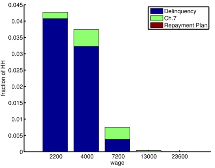
2.7 Average Repayment Decision, Repayment Plan available . . . 31
2.8 Average Repayment Decisions . . . 34
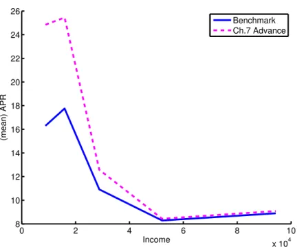
2.9 Average Credit Price by Income, Benchmark vs. Bankruptcy Advance available . . . 35
2.10 Welfare Effects, Bankruptcy Advance available . . . 37
2.A.1 Scatter Plot of Maximum APR in SCF . . . 43
2.B.1 Credit Pricing Function,q . . . 44
3.1 Annual bankruptcy filings per household, in %. . . 50
3.2 Garnishment Schedule according to German Insolvency Law (“Pfändungs-grenzenbekanntmachung 2013”). . . 58
3.3 Distribution of Bad Debt . . . 60
3.4 Labor Supply Decisions Before, During, and After Bankruptcy. . . 61
3.5 Equilibrium Loan Prices, Age 50. . . 62
3.6 Effects of Abolishing Garnishment. . . 64
3.7 “No Garnishment” versus Benchmark, by Age. . . 66
3.8 Ex-ante Welfare of “No Garnishment.” . . . 67
3.9 Effects of Optimal Garnishment Regime. . . 70
3.10 Optimal Regime versus Benchmark, by Age. . . 72
3.11 % CEV: Optimal Regime vs. Benchmark, by Income. . . 73
3.A.1 Garnishment under Alternative Policy Experiments. . . 76
3.A.2 Effects of Introducing “Mean Income Exemption.” . . . 76
3.A.3 % CEV: “Mean Income Exemption” vs. Benchmark, by Income. . . 77
List of Figures
3.A.5 % CEV: “Lenient Garnishment” vs. Benchmark, by Income. . . 78
3.B.1 Experience Profile in Monthly Wages. . . 79
4.1 Evolution of Individual Type Scores . . . 98
4.2 Evolution of Type Score Distribution . . . 99
1.1 The Importance of Unsecured Debt . . . 2
2.1 Exogenous Parameters . . . 18
2.2 Data Fit . . . 19
2.3 Estimated Parameters . . . 20
2.4 Non-Payment by 30% Lowest Income Households . . . 25
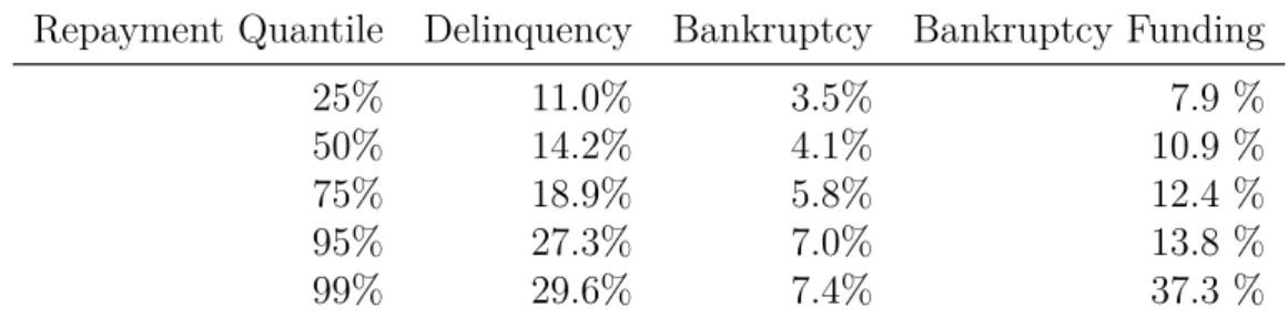
2.5 Realized Repayment Fractions, Delinquency and Bankruptcy . . . 28
2.6 Equilibrium Repayment Decisions . . . 36
2.7 Realized Repayment Fractions, Bankruptcy Advance available . . . 36
3.1 Direct Specification . . . 56
3.2 Jointly-Targeted Moments . . . 59
3.3 Internally-Determined Parameters . . . 59
3.4 Equilibrium Outcomes, Benchmark vs. “No Garnishment” . . . 65
3.5 Planner Solution . . . 69
3.6 Equilibrium Outcomes, Benchmark vs. Optimal Regime . . . 71
3.A.1 Equilibrium Outcomes, Benchmark vs. Policy Experiments . . . 75
4.1 Intermediate Cases . . . 102
4.2 Full Model with Over-Optimists and Pooling . . . 104
The behavior of individual consumptions, wealths, and portfolios is strongly at variance with the complete markets model implicit in the representative agent framework.
— Aiyagari (1994)
1 Preface
Whereas heterogeneous agent models with elaborate asset dynamics have claimed a prominent role in quantitative macroeconomics to better understand the link between wealth and income distributions and their impact on policy design, the role and evolution of debt has received relatively little attention. In the household sector, endogenous borrowing constraints, endogenous loan pricing and equilibrium default have only gained increasing attention fueled by the recent Subprime Crisis.
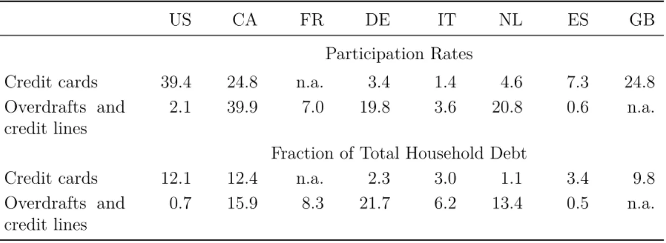
However, understanding how households use debt, why households default on their debt and how debt is priced holds genuine macroeconomic importance. In the absence of perfect financial markets, assets and debt are important tools for households to smooth consumption in the face of idiosyncratic risk. My work focuses on unsecured debt and – as presented in Table 1.1 – large fractions of households hold unsecured debt. In the U.S., more than 40% of households have some form of unsecured debt. This fraction is roughly 23% in Germany, but as high as two-thirds in Canada. Unsecured debt constitutes a significant fraction of total debt holdings. U.S. households hold roughly 13% of their debt as unsecured debt, Germans hold 24% as unsecured debt and Canadians hold nearly 30% of their debt as unsecured debt.
Default – potentially followed by debt relief – can not only provide valuable insurance for households in adverse situations; moreover, it also plays a central role when financial intermediaries price their debt. Future expected default rates are key to determining current credit price schedules. The possibility to default consequently influences all borrowers, not only those failing to service their debt.
The most important statutory way of debt relief granted to households is consumer bankruptcy. When designing consumer bankruptcy laws, policy-makers face a trade-off: on the one hand, if debts are easily forgiven, bankruptcy law grants partial insurance to those declaring bankruptcy; and on the other hand, default premia on interest rates rise in response to higher non-payment risk. This dissertation comprises three self-contained essays in which I analyze the effects of consumer bankruptcy laws on household borrowing, interest rates, default decisions, and welfare in different institutional settings.
Table 1.1: The Importance of Unsecured Debt
US CA FR DE IT NL ES GB
Participation Rates
Credit cards 39.4 24.8 n.a. 3.4 1.4 4.6 7.3 24.8
Overdrafts and
credit lines 2.1 39.9 7.0 19.8 3.6 20.8 0.6 n.a.
Fraction of Total Household Debt
Credit cards 12.1 12.4 n.a. 2.3 3.0 1.1 3.4 9.8
Overdrafts and
credit lines 0.7 15.9 8.3 21.7 6.2 13.4 0.5 n.a.
Source: Campbell (2016, Tables 1 and 2)
Chapter 2 analyzes whether and how to regulate small dollar lending in the U.S. For
this purpose, I develop a structural model of unsecured lending where heterogeneous households can not only file for bankruptcy but also become delinquent. Introducing fixed cost of loan creation endogenously produces realistic interest rates of up to 300% for small loans. In the face of income and expenditure risk, households can partially insure through bankruptcy, which provides legally mandated debt relief. However, lump sum court fees and lawyer costs prevent low-income households from filing for bankruptcy protection. Without access to bankruptcy, these households become delinquent and pay late fees to avoid collection efforts from their banks. My quantitative results show that delinquency offers insufficient insurance against adverse events, granting room for welfare-improving policy interventions. In one such intervention, low-income households are allowed to repay bankruptcy filing costs after debt relief, making bankruptcy more affordable. I show that bankruptcy filings increase and delinquency decreases. Low-income households enjoy a 1% welfare increase, while aggregate welfare increases by 0.1%. The repayment plan
proposed by the Consumer Financial Protection Bureau – which allows households to spread repayment over three periods – does not yield any welfare gains.
Chapter 3 evaluates the German bankruptcy system, which features relatively harsh
wage garnishment. While the U.S. regime has a strong insurance component, many European systems are stricter in that they force delinquent households to repay (parts of) the outstanding debt through wage garnishment. Since wage garnishment raises the effective marginal tax rate, it exhibits adverse effects on labor supply. Explicitly modeling labor supply, this paper examines the optimal garnishment regime for the German economy and the resulting impact on credit prices. Under the optimal garnishment regime,
garnishment rates are reduced by more than 25%, while the duration of garnishment is increased from six to ten years. This results in an aggregate welfare increase of around 3.3%. Low-income households gain up to 7% since they have significantly better access to cheaper credit, which allows them to better smooth consumption over the life-cycle. High-income households already face favorable credit conditions and thus only gain 0.8%. Fully removing wage garnishment and moving to a “Fresh Start” regime similar to the U.S. raises the price of credit since lenders internalize the possibility of not being paid back. Young households suffer from restricted access to credit and the welfare of newborns decreases by roughly one percent.
Chapter 4 is joint work with Igor Livshits,1 James MacGee,2 and Michèle Tertilt.3
There is increased debate over whether the regulation of unsecured consumer lending products is required to protect some consumers from “over-borrowing.” To assess the quantitative benefits of regulating the cost of declaring consumer bankruptcy, we analyze a life-cycle model where some consumers have excessively optimistic beliefs about their exposure to unforeseen expenses. Building on Livshits, MacGee, and Tertilt (2010), we examine a heterogeneous agent incomplete market life-cycle model with bankruptcy. Over-optimists persistently believe that they face the same risks as realists, even though they are exposed to fundamentally higher expense risk. Competitive lenders are unable to directly distinguish between over-optimists and realists. However, they can observe a consumer’s present income, debt level and history of defaults. Lenders use this information to form a type score that represents the probability of whether a consumer is an over-optimistic or realist type. This results in partially pooling different types of households to whom lenders assign the same type score. Since lenders incorporate expected default risk in the bond price schedules that they quote consumers, over-optimistic households face lower interest rates and borrow more when they are pooled with realists. The opposite is true for realists. We calibrate the model to match aggregate bankruptcy filing rates, unsecured debt to income and average borrowing interest rates in the U.S. Using the calibrated model, we show that especially over-optimistic households suffer from a policy that introduces higher repayment requirements for households filing for bankruptcy.
1Federal Reserve Bank of Philadelphia and BEROC. The views expressed here are those of the authors
and do not represent those of the Federal Reserve Bank of Philadelphia or the Federal Reserve System.
2University of Western Ontario. 3University of Mannheim and CEPR.
2 Regulating Small Dollar Loans:
The Role of Delinquency
2.1 Introduction
Small, short-term loans are an important source of liquidity for many households. Espe-cially sub-prime, low income households have little or no access to mainstream sources of credit such as credit cards or bank overdraft. Hence, financially constrained households turn to payday loans, deposit advance products, and other small dollar loans to gain access to credit. These loans are usually short-term, relatively small, and very expensive. Payday loans for example are due after two to four weeks and usually amount to less than $1,000. Interest rates as high as 20% per loan amount to annualized percentage rates
(APRs) of up to 700%. Despite being very expensive, payday loans constitute a sizable market in the United States. Annual lending of $50 billion creates $8 billion in interest payments. About 12 million borrowers use payday loans each year. Although intended to provide short-term liquidity, payday loan users roll over increasing amounts of debt many times. More than 15% of loans are rolled over at least ten times.
High prices and numerous roll-overs sparked a lively policy debate on how to regulate small dollar loans. Current state-level legislation spans from not regulating small dollar loans at all to prohibiting small dollar loans completely.1 Nationwide regulation is absent,
but the recently established Consumer Financial Protection Bureau (CFPB) has just proposed a first attempt to regulate such loans.2 The CFPB argues that small dollar
loans are “consumer debt traps” not only because of their exorbitantly high price but also because fees, interest payments and the principal are all due in one balloon payment, which is unlikely to be paid back in full.3 Some consumer agencies contend that unaffordable
balloon payments form an essential part of the business model of small dollar lenders. To
1For an overview of current state-level legislation, please see http://www.pewtrusts.org/en/
multimedia/data-visualizations/2014/state-payday-loan-regulation-and-usage-rates.
2Small dollar lenders are of course subject to other, more general regulation applicable to any commercial
credit supplier such as the Fair Credit Reporting Act or the Truth in Lending Act.
3The full text of the proposal is available at
http://files.consumerfinance.gov/f/documents/
that end, lenders allegedly provide loans that households can never repay in full. Keeping households in debt, these lenders are presumed to generate profit through repeatedly charging late fees for unpaid loans.4 In an other line of argument, Pew Charitable Trusts
(2013) is concerned that borrowers do not fully understand the contracts they are offered. However, the rationale for regulation remains unclear: While prices may be high, small dollar loans are effectively the only tool to smooth consumption that is available to low-income households.
I provide a structural framework to quantify the trade-off between partial insurance obtained through bankruptcy or delinquency and increasing credit prices in the small dollar lending market, both for low-income households and the economy in aggregate. The calibrated model is used to answer the question of whether and how to regulate small dollar loans. Risk-averse households borrow from risk-neutral banks, who accept deposits at the risk-free rate but issue debt at state-contingent prices. Households cannot commit on repaying outstanding debt. Consequently, default arises in equilibrium. In particular, households can use two types of nonpayment to partially insure against idiosyncratic risk: bankruptcy or delinquency. When households cannot afford bankruptcy filing fees, they become delinquent on their debt. Unlike bankruptcy, delinquency does not offer debt relief. Furthermore, delinquent households are subject to collection efforts by their lenders. Delinquency thus provides only limited insurance which means little opportunity to smooth consumption across states.
Contrary to the ongoing policy discussion, the underlying inefficiency in the small dollar loan market does not stem from the size of repayments, but from insufficient risk sharing while in delinquency. In the spirit of Aiyagari (1994), Bewley (1986), and Huggett (1993), households face idiosyncratic risk that is not directly insurable in the market. By introducing some state contingency to debt contracts, default can potentially increase welfare (c.f. Zame, 1993). In the United States, Chapter 7 bankruptcy provides households with an opportunity of debt relief. But filing for bankruptcy involves paying significant filing fees such as lawyer fees and court fees. Low income households, who are typical borrowers in the small dollar loan market, consequently cannot afford to file for bankruptcy. For these households, the only way to insure against income or expenditure risk is to become delinquent. Some households are “trapped” in debt long enough to repay more than they originally owed. That means that the unluckiest households can insure the least.
In order to provide better insurance for low income households, I introduce a bankruptcy advance for those households unable to pay the filing fees. Households using a bankruptcy
4See, for example,
http://www.pewtrusts.org/en/research-and-analysis/issue-briefs/2014/
2.1 Introduction advance can file for bankruptcy, gain debt relief and only later repay the lump sum costs. Since low income households gain the outside option of walking away from their debt, delinquency becomes less harsh along both the extensive and intensive margin: Delinquencies drop by two thirds, and conditional on delinquency, banks extract less resources. Both effects increase the amount of insurance low income households can access. As a result, these households enjoy a 1% gain in consumption-equivalent welfare. Over all income groups, welfare increases by 0.1% on average with no group becoming worse-off
due to the reform.
To evaluate the policy proposal put forward by the CFPB, a repayment plan is introduced in the economy. It is supposed to make repaying small dollar loans easier. Instead of repaying all debt in one large balloon payment, the plan spreads repayment over three periods. When using this plan, households cannot borrow on other small dollar loans. The proposal does not work; I find that households never opt into the repayment plan. In good times, households prefer to repay directly in order to retain the flexibility of choosing future debt or asset positions after learning about future income and unforeseen expenditures. In bad times, the repayment plan is not affordable and low income households still resort to delinquency.
I contribute to the consumer bankruptcy literature along two dimensions: Firstly, I add delinquency as a realistic nonpayment choice when bankruptcy is not affordable. Subject to limited commitment, banks try to optimally extract resources from delinquent borrowers. This mechanism makes delinquency especially harsh on households that do not have the outside option of officially filing for Chapter 7 bankruptcy protection. Secondly, I include per loan fixed cost when banks originate loans in a competitive market. These fixed costs generate realistically high interest rates for small loans.
To my knowledge, this paper is the first to provide a quantitative analysis of the small dollar loan market. There are some papers, however, that attempt to document the impact that payday loans have on households’ financial well being. Payday loans are the most prevalent form of small dollar loans. On the one hand, Morgan, Strain, and Seblani (2012) and Zinman (2010) document that payday loans help households to smooth consumption. On the other hand, Melzer (2011) and Skiba and Tobacman (2011) provide evidence that using payday loans makes households less likely to repay outstanding financial obligations. The payday lending market seems to be an alternative to mainstream lending through credit cards and overdraft. Using data from a payday lender matched to credit histories, Bhutta, Skiba, and Tobacman (2015) find that mainly financially constrained households take out payday loans. For a proper welfare analysis, however, it is necessary to structurally model how household choices and equilibrium outcomes influence household utility.
Notwithstanding, there exists a large empirical literature documenting important facts of the payday lending market. Although intended to provide short-term liquidity, payday loan users roll over increasing amounts of debt many times. More than 60% of newly created loans are rolled over at least once, while 15% of loans are rolled over at least ten times (Burke, Lanning, Leary, and Wang, 2013).
Flannery and Samolyk (2005) and Skiba and Tobacman (2007) provide evidence on the importance of fixed cost of loan creation. Even though prices are very high, payday lenders do not earn excess profits when compared to other lenders such as credit card companies. Rather than market power, per-loan fixed cost drive up prices for small short-term loans. Ernst and Young (2004) calculates that of the total cost in the payday lending industry, 75% are fixed cost while 20% are due to nonpayment.
Despite typically carrying three digit interest rates, small dollar loans are generated employing similar technology as larger unsecured loans. When comparing variable costs, small dollar loan businesses face costs of funds very similar to credit card lenders. In terms of per loan fixed cost, Stango (2012a) highlights that while absolute fixed costs per loan are comparable, fixed costs relative to loan size are much larger in the small dollar lending market simply because of smaller loan sizes. Mechanically, fixed costs per dollar lent decrease in the size of the loan.
Bankruptcy filing costs can be prohibitively high for low-income households. Using the increase in bankruptcy filing costs after the 2005 BAPCPA reform, Albanesi and Nosal (2015) document that low-income households remain delinquent longer and file for Chapter 7 bankruptcy less often. High-income households are not affected by the increase in filing cost. Similarly, Mann and Porter (2009) document that liquidity constraints bar low income households from filing for Chapter 7 bankruptcy. Gross, Notowidigdo, and Wang (2014) show that increased liquidity from tax rebates increases bankruptcy filings.
Households in my model behave rationally and are fully aware of the high costs of small loans. While this assumptions abstracts from problems when borrowers do not fully understand the contracts they are offered, there is little evidence for this. Bertrand and Morse (2011) find that only 10% of borrowers react to information treatments right before taking out payday loans. All other borrowers understand the cost of borrowing and do not adapt loan sizes at all. Using administrative data on an experiment conducted by a large American bank, Agarwal, Chomsisengphet, Liu, and Souleles (2015) find that borrowers correctly choose the credit contract that minimizes their cost on average.
I set up a quantitative limited commitment model of unsecured debt that features both, official Chapter 7 bankruptcy and delinquency. My model extends quantitative models of consumer bankruptcy, most notably Chatterjee, Corbae, Nakajima, and Ríos-Rull (2007) and Livshits, MacGee, and Tertilt (2007). Most models focus on bankruptcy
2.2 Model as the only nonpayment option, while I include the additional option of delinquency. Quantitative models of bankruptcy have been used to analyze many important policy questions: Mitman (2016) analyzes the interplay between bankruptcy and mortgage default regulation. Chatterjee and Gordon (2012) compare the welfare effects of bankruptcy protection vis-à-vis creditors directly garnishing income. Exler (2016) analyses how to reform income garnishment as a part of official consumer bankruptcy in Germany. Bankruptcy also provides insurance to potential entrepreneurs, see Akyol and Athreya (2011) and Mankart and Rodano (2015) for a setup with secured credit.
Athreya, Sánchez, Tam, and Young (2015) are most closely related to my setup. They also allow borrowers to informally default by simply not repaying and, hence, becoming delinquent on outstanding debt. Athreya, Sánchez, Tam, and Young document that a model with formal default through bankruptcy and informal default through delinquency does well in matching observed consumer credit patterns. I depart from their setup in two ways: (1) I introduce fixed cost in loan creation which produce realistic credit prices for small dollar loans. (2) I allow banks to optimally exploit the hold-up situation that arises after a household becomes delinquent. Banks can not only restructure the loan but also charge optimal late fees. This is not only a realistic assumption but also crucial to the amount of insurance delinquency provides. Households with no (or low) outside options are treated more harshly in delinquency than households that might simply file for bankruptcy. Furthermore, Herkenhoff (2012) employs a search framework to analyze partial repayment as a means of informal unemployment insurance. In Herkenhoff’s setup, households choose which fraction of debt to repay in order to insure against separation shocks.
The remainder of this paper is structured as follows: Section 2.2 presents the model. The calibration is discussed in Section 2.3. Section 2.4 describes the trade-off between bankruptcy and delinquency and documents that delinquency might “trap” unlucky households in debt. Subsequently, a repayment plan is introduced and the results of this policy experiment are discussed (Section 2.5). Section 2.6 describes the effects of introducing a bankruptcy advance. Section 2.7 concludes.
2.2 Model
The economy is populated by a continuum of infinitely lived households. Subject to individual earnings and expenditure risk, households maximize utility by choosing con-sumption and savings. Besides just repaying outstanding debt, individuals can choose to file for Chapter 7 bankruptcy or simply choose not to repay. In the latter case, they
become delinquent on their debt.
Financial intermediaries operate in a perfectly competitive market. They offer loan contracts dependent on loan size and household characteristics, subject to variable cost and fixed cost of loan creation. In the case of delinquency, banks maximize expected recovery by optimally choosing to levy late fees and restructure the loan contract.
2.2.1 Household Problem
The household state is fully described by individual asset holdings (at, where at<0 is
debt), individual earnings (et) and individual expenditure shock (κt). Earnings consist of
a persistent component (zt, modeled as an AR(1) process) and a transitory component
(εt, modeled as white noise). See Equation (2.8) for details. Expenditure shocks represent
unforeseen expenditures that strain a household’s budget. They represent expenditures as caused by marital disruptions, the replacement of durables and large health care bills. These shocks are assumed to be uncorrelated across time.5 For brevity of notation, I
will summarize the exogenous household states asst= (zt, εt, κt) such that the full state
simply reads (at, st).
Households choose the sequence {ct, pt, at+1}∞t=0 of consumption ct, repayment modept
and next period asset holdings at+1 to maximize the discounted sum of expected utilities E ∞ P t=0 βtu(c t)|a0, s0
. Here, u(c) =c1−ρ/(1−ρ) is a standard utility function featuring
constant relative risk aversion. The problem is presented in recursive formulation, where
x0 denotes the next period value of a variable x.
In each period, solvent households
1. observe their idiosyncratic earnings e, expenditure shock κ and assets a,
2. optimally choose whether to stay solvent (p(s, a) =S), file for Chapter 7 bankruptcy
(p(s, a) =B) or become delinquent (p(s, a) = D) and
3. choose consumption (c(s, a)) and savings (i.e. next period’s asset holdings, a0(s, a))
optimally.
5This specification is standard in the consumer bankruptcy literature, see Livshits, MacGee, and Tertilt
(2007, 2010). Unforeseen expenditures are frequently quoted as an important reason for default. Not paying unsecured loans (e.g. through filing for bankruptcy) thus partially insures households against these risks.
2.2 Model
Solvency
The value of solvency (VS) is presented in Equation (2.1):
VS(a, s) = max c,a0 [u(c) +βEsV(a 0 , s0)] s.t. c+q(a0, s)a0 =e+a−κ, (2.1) where Es denotes the expectation of next period’s value conditional on the current
household state s. The budget constraint in solvency simply states that expenditures
(consumption plus next period wealth) cannot exceed earnings (e) plus initial wealth (a)
minus the expenditure shock (κ). q(·) denotes the bond price households are offered for
saving or borrowing. q(·) represents the inverse of one plus the interest rate.
Bankruptcy
If choosing to file for Chapter 7 bankruptcy, households have to pay lump-sum costs F
and additionally suffer utility costζB. Since individuals can neither save nor borrow in the
period of filing for Chapter 7 bankruptcy, they simply consume their endowment minus monetary filing costs. In the period following bankruptcy, all debt is forgiven (a0 = 0)
and there are no further repercussions. Hence, next period’s value reads V(0, s0). The
value from filing for bankruptcy protection thus is
VB(a, s) =u(e−F)−ζB+βEsV(0, s0). (2.2)
Assuming that individuals do not face negative consequences following a Chapter 7 bankruptcy abstracts from possible effects of bankruptcy on a household’s credit report. This is not a strong assumption, as Bhutta, Skiba, and Tobacman (2015) show that credit scores typically are not affected by filing for bankruptcy (but rather by previous failures to repay). Even low income bankrupts are not excluded from unsecured lending: Cohen-Cole, Duygan-Bump, and Montoriol-Garriga (2009) document that specialized lenders target unsecured credit at lower income households just after Chapter 7 bankruptcy. Additionally, Han and G. Li (2011) document that households still use small dollar loans after filing for bankruptcy. These loans are generated using sub-prime credit scores that do not respond to bankruptcy flags, either (Bhutta, Skiba, and Tobacman, 2015).
All remaining negative consequences of declaring bankruptcy are assumed to be captured byζB. It is supposed to represent stigma of filing for bankruptcy and other adverse effects
outside the model such as difficulties when renting an apartment or signing up for phone contracts.
Filing costsF represent out-of-pocket expenses necessary to cover lawyer fees and court
fees and have to be paid upfront when filing for Chapter 7. Due to these fees, filing for bankruptcy is very painful if not infeasible for low income households. Even if filing fees do not exceed labor income, the utility of forgone consumption for low income households is very high (due to the concavity of the utility function). Explicitly modeling lump-sum filing cost hence allows me to capture the fact that low income households are less likely to file for bankruptcy and rather stay delinquent. This observation is documented by Albanesi and Nosal (2015). Albanesi and Nosal find that increased monetary filing cost after the 2005 bankruptcy reform reduced Chapter 7 bankruptcies. This drop in bankruptcy filings leads to an increase in delinquencies. The effect is found to be most dominant for low income households.
Delinquency
If households choose to neither repay outstanding loans nor to officially file for bankruptcy, they become delinquent on their debt.6 In that case, creditors can restructure the
outstanding loan and charge a late fee. Since I assume limited commitment, households cannot be forced to pay these fees, though. If households decide not to pay (ν(s, a) = 0),
households suffer collection efforts that create a utility loss. Payment of late fees arises endogenously, if households are better off paying the proposed fees than suffering collection efforts.
There are many legal ways for lenders to employ collection in order to inflict utility costs on borrowers: letters threatening legal consequences, calls to the debtors, the debtors’ employers or the debtors’ family members or in-person visits. Furthermore, payday lenders in particular threaten to cash the borrower’s post-dated check that was signed at origination. This would inflict further financial stress in the form of overdraft fees with the borrower’s bank, for example. Additionally, one might argue that some lenders also employ collection efforts outside the law.7
6To my knowledge, there is only one other paper that formally models delinquency. I depart from
Athreya, Sánchez, Tam, and Young (2015)’s setup in allowing banks to recover as much as possible of any delinquent loan. In my setup, banks optimally levy late fees and restructure delinquent loans, subject to limited commitment on the household side. This is crucial when analyzing possible policy reforms since banks take advantage of the missing outside option of Chapter 7 bankruptcy for low income households. See Section 2.2.2 for more details.
7See Hunt (2007) for an overview of debt collection practices in the US. Drozd and Serrano-Padial
(2015, Appendix 1) provide detailed information on the influence of information technology on collection. The CFPB collects complaints about collection efforts that are perceived to exceed the legal boundaries set by the Fair Debt Collection Practices Act. For the full data, seehttps:
2.2 Model
VD defines the value of delinquency as
VD(a, s) = max c,ν [u(c)−(1−ν)ζD+βEsV(α(a 0 , s0), s0)] s.t. c=e−νL(s) ν ∈ {0,1}. (2.3)
In delinquency, households choose how much to consume and whether to pay late fees (ν(a, s) = 1) or not (ν(a, s) = 0). If households do not pay late fees L(s), they suffer
collection efforts that induce a utility cost ofζD.
In contrast to bankruptcy, delinquent debt is not written off by law. Since lenders are free to restructure delinquent debt contracts, next period’s debt holdings are set to
α(a0, s0). The intermediaries’ problem of optimally setting L(s) and α(a0, s0) is described
in Section (2.2.2).
Complete Household Problem
The full household problem at the beginning of each period can be presented as
V(a, s) = max
p∈{S,B,D}V
p(a, s). (2.4)
After observing the period’s state (a, s), households choose the payment modep(·) that
maximizes V(a, s). Households choose between solvency (p=S), filing for bankruptcy
(p=B) and delinquency (p=D). The corresponding Value Functions VS, VB andVD
are presented above, in Equations (2.1), (2.2) and (2.3). Note that, in certain states, some repayment modes might be infeasible. In particular, solvency is not feasible if income is sufficiently low or expenditure shocks are sufficiently high. Additionally, if income is lower than the lump-sum Chapter 7 filing costs, bankruptcy yields an empty budget set. I set the utility of empty budget sets to u(c ≤ 0) = −∞. In these cases, delinquency
(p(·) =D) is the only feasible alternative.
2.2.2 Banking Sector
The banking sector is assumed to be perfectly competitive with free entry and exit. Hence, banks price loans competitively, expecting zero profit for each contract offered. They can refinance externally, at the risk-free interest rate r. For each loan size and household
state, banks form expectations over the probability of repayment and possible losses either because borrowers file for bankruptcy or because households become delinquent.
Debt Pricing Function
The pricing function is a function of the loan size and the household state when taking out a one-period loan. Both, a0 and s, govern the probability and size of repayment. Savings,
on the other hand, are not risky and earn the risk free rate:
q(a0, s) = (1 +r)−1 ∀a0 ≥0. (2.5)
When creating loans, financial intermediaries face two types of transaction costs: fixed cost δ and variable (proportional) cost γ. These cost capture fixed per loan expenses such
as labor cost of initiating a loan contract as well as variable operating expenses such as billing, payment processing and administration (c.f. Agarwal, Chomsisengphet, Mahoney, and Stroebel, 2015).
To my knowledge, this paper is the first paper in the consumer bankruptcy literature to introduce per loan fixed cost into debt pricing models. In the absence of market power, fixed cost are important to realistically capture the high prices observed for small loans.8
In standard models without fixed cost, interest rates only increase if default risk increases. In other words, credit spreads can only arise due to nonpayment risk. In order to capture the observed interest rates for small loans, nonpayment risk would thus have to be very large. In reality however, nonpayment risk only constitutes 30% of credit spreads that are observed in the data (Skiba and Tobacman, 2007).
Let ¯q = (1 +r+γ)−1 denote the lender’s (constant) marginal cost of generating loans.
Then, a risk-free loan of size ˜a0 would face the price
q(˜a0, s) = ¯q− δ
˜
a0.
That means that households would receive a loan of sizeq(˜a0, s)˜a0 = ¯q˜a0−δ and repay the
face value of ˜a0 next period. Consequently, if q(·)→0, the implicit interest rate on that
loan approaches infinity. Vice versa, if q(·)→1, the implicit interest rate on that loan
approaches 0.
In equilibrium, bankruptcies and delinquencies occur and repayment is not certain. When banks take borrowers’ nonpayment decisions into account, risky loan prices evolve
8See Ernst and Young (2004) and Flannery and Samolyk (2005) for empirical evidence on the
competi-tiveness of the small dollar lending market and further evidence on the importance of per loan fixed cost in the small dollar loan market.
2.2 Model according to q(a0, s) = ¯q E[IS(a0, s0)|s]·1 +E[IB(a0, s0)|s]·0 +E " ID(a0, s0) R(a0, s0) |a0| |s #! − δ |a0|, (2.6)
where E[θ(a0, s0)p |s] denotes the conditional probability of a household in states that
receives a loan of sizea0 to choose repayment mode p next period.
In the case of solvency (IS(·) = 1), banks are repaid in full, hence the first line in
Equation (2.6) is multiplied by 1. When filing for bankruptcy (IB(·) = 1) though, banks
retrieve nothing, hence these cases are multiplied by 0. Finally, when households become delinquent (ID(·) = 1), banks recoverR(a0, s0), as will be described in Problem (2.7). For
a loan of sizea0, financial intermediaries thus expect to recover the fraction R(a0, s0)/|a0|
in delinquency.
Optimal Recovery in Delinquency
If households become delinquent on a loan, banks can charge late feesL(s) and restructure
the loan to hold a face value of α(a, s) next period. When charging fees, banks take
into account the limited commitment of households which can always choose not to pay. Hence, the utility cost of nonpayment restricts the amount of fees banks can charge in a given period.
When restructuring, banks are free to reduce the face value of the loan, subject to the households’ repayment behavior. That means banks can, on the one hand, decrease the payable amount to incentivize households to repay. On the other hand, banks can keep the payable amount as is in order to make repayment less likely and extract more resources from debtors through fees. Restructuring loans amounts to banks optimally adapting the size of outstanding debt, subject to the risky loan price schedule. Hence, banks set late fees (L) and reset the outstanding loan to size α to maximize expected
repayment. They solve the problem
R(a, s) = max L,α L+q·(−α) s.t. u(e−L)≥u(e)−ζD q=q(α, s0) α≥a0. (2.7)
Problem (2.7) states that, conditional on delinquency, banks maximize current and expected future returns. In choosing late fees and next period’s face value optimally, banks are subject to limited commitment on the household side in two ways: Firstly, households can choose to not pay any fees and rather suffer the utility cost ζD resulting
from collection efforts. Hence, banks can only levy fees up to an amount that makes households indifferent between paying and not paying (u(e−L)≥u(e)−ζD). Secondly,
setting next period’s face value, banks take into account that household can always choose between repayment, bankruptcy or delinquency. Banks thus discount next period’s face value α with the risky rate q(·). As described above, q(α, s0) reflects the household’s
expected repayment behavior in the following period, given the reset face value and the observed household state.
Finally, I assume that banks are not allowed to increase outstanding debts, henceα ≥a0.
Otherwise, for some incomes, it might be optimal to set α → −∞ in order to ensure
delinquency and thus late fee payment in all future states of the world (except when bankruptcy becomes available due to a steep increase in income). This is neither legal nor observable in reality, hence I restrict restructured debt α to be weakly less than the
original amount owed.
Small Dollar Loans are issued employing the same technology as other unsecured loans. Since these loans are typically smaller than other unsecured credit, per loan fixed cost have a larger effect on their price. Loans carrying APRs in excess of 30% or loans not exceeding the amount of $1,000 are interpreted as Small Dollar Loans. This definition
will be discussed in detail in Section 2.3.2.
2.2.3 Equilibrium
Given a risk-free rate r and an income process e, a financial market equilibrium is the
set of value functions V, VS, VB and VD, policy functions c(·), a0(·), p(·), conditional
repayment probabilities E[Ip(·)|s], p∈ {S, B, D}, a recovery functionR(·) and a debt
pricing function q(·) such that:
1. Households maximize V, VS, VB and VD, where c(a, s), a0(a, s), p(a, s) are the resulting optimal policy functions.
2. The bond priceq(a0, s) is determined in a competitive market with free entry, taking
as given the expected default behavior E[Ip(a0, s0)|s] and the expected recovery in
delinquency E[R(a0, s0)|a0, s].
2.3 Calibration
2.3 Calibration
The model has 16 free parameters of which nine are set exogenously. The remaining seven parameters are jointly determined in order to match important data moments. These moments describe the United States’ economy after the recent financial crisis.
2.3.1 Direct Specification
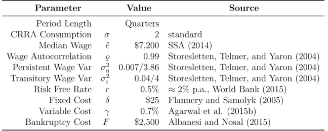
In order to capture the typical short duration of small dollar loans, the period length of the model is set to quarters. Households’ coefficient of relative risk aversion is set to a standard value ofσ = 2.
The income process e = ˆe·y represents idiosyncratic income that households earn.
It has a constant component ˆe that represents the median endowment in the economy.
Additionally, y represents idiosyncratic income risk that households face. It is defined
as the residual of regressing household income on observables such as age and education. Following standard assumptions in the literature, it is composed of a persistent AR(1) process zi,t and transitory white noiseεi,t. For household i at timet it is given by
log (yi,t) =zi,t+εi,t
zi,t =%zi,t−1+ηi,t,
(2.8) where %∈[0,1],ε∼N(0, σ2ε) and η ∼N(0, ση2). Using data from the PSID, Storesletten,
Telmer, and Yaron (2004) estimate the auto correlation coefficient % and the standard
deviations ofεandη. I convert their values to quarterly values. To that end, I assume that
Storesletten, Telmer, and Yaron’s annual process is the result of aggregating a quarterly income process. I report the quarterly values in Table 2.1. Median quarterly income is set to ˆe = $7,200 as reported by the Social Security Administration (SSA).9
The risk-free interest rate at which banks can refinance externally is set to r = 0.5%
quarterly. This roughly translates to an annual real interest rate of 2%.10 Transaction
cost for creating loans are set toγ = 0.7%, which corresponds to roughly 3% p.a. and is in
line with the operational cost of 3.4% estimated by Agarwal, Chomsisengphet, Mahoney,
and Stroebel (2015). Lending fixed cost are set to δ= $25, as documented by Flannery
and Samolyk (2005).
Out-of-pocket expenses when filing for bankruptcy (F) are set to $2,500, following the
analysis by Albanesi and Nosal (2015). These expenses comprise of court fees and lawyer fees, both of which are unavoidable if a household files for Chapter 7 bankruptcy.
9See
https://www.ssa.gov/oact/cola/central.html.
10See
Table 2.1: Exogenous Parameters
Parameter Value Source
Period Length Quarters
CRRA Consumption σ 2 standard
Median Wage eˆ $7,200 SSA (2014)
Wage Autocorrelation % 0.99 Storesletten, Telmer, and Yaron (2004)
Persistent Wage Var σ2
η 0.007/3.86 Storesletten, Telmer, and Yaron (2004)
Transitory Wage Var σ2
ε 0.04/4 Storesletten, Telmer, and Yaron (2004)
Risk Free Rate r 0.5% ≈2% p.a., World Bank (2015)
Fixed Cost δ $25 Flannery and Samolyk (2005)
Variable Cost γ 0.7% Agarwal et al. (2015b)
Bankruptcy Cost F $2,500 Albanesi and Nosal (2015)
2.3.2 Simulated Method of Moments
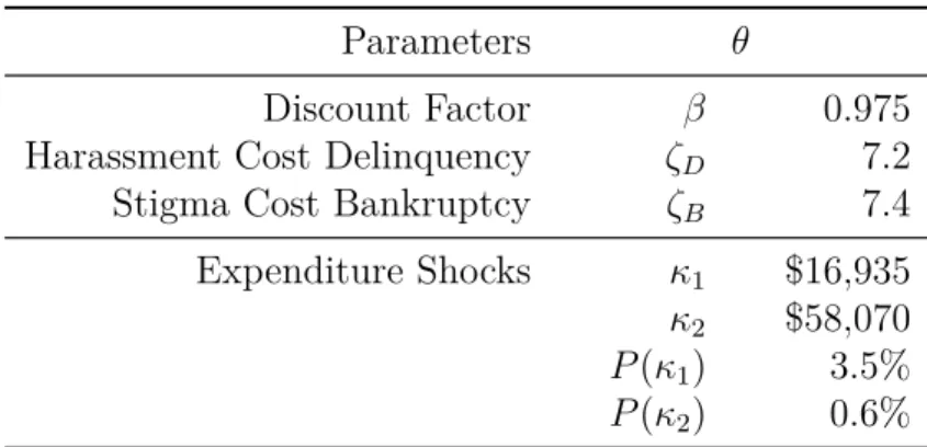
After setting nine parameters exogenously, seven parameters remain to be determined jointly. There are three utility parameters: the discount rate (β), the harassment cost
in delinquency (ζD) and stigma cost of bankruptcy (ζB). Following Livshits, MacGee,
and Tertilt (2010), I assume the expenditure shock to take two non-zero values. Hence, there are four additional parameters: two parameters governing the size (κ1, κ2 and
two parameters governing the respective realization probabilities (P(κ1), P(κ2)). These
parameters (summarized by θ) are set to minimize the percentage deviations between
model moments and data
min θ X i Mi(θ) Di −1 !2 . (2.9)
Here,Mi(θ), i ={1, . . . ,7} represent seven model moments as a function of the seven free
parameters θ. Di, i={1, . . . ,7} represent the corresponding data moments. The model
and data moments are reported in Table 2.2; Table 2.3 presents the parameter estimates. The debt to income ratio for unsecured debt relative to quarterly household income of roughly 35% is slightly overestimated by the model. On the other hand, the fraction of households holding debt is underestimated. The model captures equilibrium delinquencies and bankruptcies well, with 1.2% of households being delinquent in any given quarter
and 0.3% of households declaring bankruptcy per quarter.
Following the empirical evidence presented in Ernst and Young (2004), Skiba and Tobacman (2007), and Stango (2012a), my model features one lending technology to generate unsecured credit. I use two definitions to define small dollar loans: Firstly, Small Dollar Loans are defined as all loans featuring APRs higher than 30%. Credit cards, which provide the main source of unsecured debt in the US, almost always have rates
2.3 Calibration
Table 2.2: Data Fit
Model Data Source
Avg. Debt/Income 35.6% 28.9% SCF (2013) Fraction of HH in debt 19.1% 37.7% SCF (2013)
Delinquencies 1.2% 1.7% FRBNY/Equifax Bankruptcies 0.3% 0.3% SCF (2013) Small Dollar Loan APR (1) 128% 300% Skiba et al., 2007
(2) 121%
Credit Card APR (1) 12.7% 17.5% Stango et al., 2016 (2) 12.5%
Default Premium 33.1% 30% Skiba et al., 2007
Note: All moments represent quarterly values. SCF (2013) are the author’s calculation. Average debt to income is the average of each household’s ratio of unsecured debt holdings relative to quarterly household income. Fraction of households in debt is the fraction of households that hold any positive amount of unsecured debt. See Appendix 2.A for more details on the calculation of these moments. The default premium is defined as the credit price spread due to default risk (in contrast to the spread due to lending costs). FRBNY/Equifax is the Federal Reserve Bank of New York’s “Consumer Credit Panel / Equifax” data as estimated by Athreya, Sánchez, Tam, and Young (2015).
lower than 30%. Using a large administrative data set, Stango and Zinman (2016, Table 2) documents that 90% of revolving credit card balances feature APRs of less than 28%. Hence, a cut-off of 30% seems reasonable. Secondly, all loans smaller than $1,000 are
defined as small dollar loans. According to Skiba and Tobacman (2008), payday loans generally do not exceed this size. When calibrating the model, I will show statistics using both definitions:
(1) APR:All loans featuring APRs higher than 30% are defined as small dollar loans.
(2) Size: All loans smaller than $1,000 are defined as small dollar loans.
In the calibration, I target the APR-based definition (1). I also report the APRs generated when using definition (2) in order to show that I am indeed capturing small loans that carry interest rates in excess of 30%.
Featuring realistic fixed cost of loan creation, the model is able to partially capture high APRs observed in the small dollar lending market according to both definitions presented above. Even though my framework falls short in terms of magnitude, it provides a much better fit than setups without any fixed cost in lending. These setups typically produce very low interest rates for the smallest loans.
Also due to fixed cost of loan creation, the model is able to match the default premium of credit prices very well (33% vs. 30% in the data). The default premium is defined as
Table 2.3: Estimated Parameters
Parameters θ
Discount Factor β 0.975
Harassment Cost Delinquency ζD 7.2
Stigma Cost Bankruptcy ζB 7.4
Expenditure Shocks κ1 $16,935
κ2 $58,070
P(κ1) 3.5%
P(κ2) 0.6%
the fraction of credit spreads that arises due to nonpayment risk rather than operating cost. In models without any fixed cost in lending, risk based credit spreads account for nearly 100% of credit spreads, since only variable lending costs (i.e. costs of funds) drive a small wedge between the risk free rate and the borrowing interest rate.
Finally, credit card interest rates are matched reasonably well according to both definitions. They remain slightly too low, though.
The endogenous parameters to to generate these moments are shown in Table 2.3. The discount factor is β = 0.975. Utility cost in delinquency and bankruptcy are 7.2 and
7.4. In terms of dollar values, these correspond to the utility loss induced by reducing a
median income household’s assets from $0 to −$30.000. Since households in the lowest
income bin have much higher marginal utility, this amount is only −$2.800 for them.
The expenditure shocks estimated in the simulated method of moments are smaller but more likely than those estimated in Livshits, MacGee, and Tertilt (2010). Since these shocks are assumed to be i.i.d., the expected realization per period is simplyP
i=1,2P(κi)κi.
In my calibration, households are on average hit by unforeseen expenditures that amount to 13% of median income whereas households in Livshits, MacGee, and Tertilt on average have to cover 40% of median income. This is mainly because Livshits, MacGee, and Tertilt feature a very large health shock that exceeds the large shock in Table 2.3 by an order of magnitude.
2.3.3 Untargeted Moments
This section compares the model to data along non-targeted dimensions. I document cross-sections of credit prices with respect to loan size and borrowers’ income. Fixed cost of loan creation generate credit prices that match the cross-section of the data well. The model can thus be used to derive reliable implications when analyzing two potential policy reforms in the following sections.
2.3 Calibration 10 15 20 25 30 (mean) APR 1 2 3 4 5 5 quantiles of size meanAPR_CCsum_bysizequant_5 (a) Data (SCF, 2013) 1 2 3 4 5 8 10 12 14 16 18 20
Loan Size Quintiles
(mean) APR
(b) Model
Figure 2.1: Average Credit Prices (APR), by loan size
Even though not directly targeted in the calibration, the model produces realistic price schedules for small dollar loans. Fixed cost of loan creation drive up interest rates for small loans, even in the absence of default risk. In standard models without fixed cost of loan creation, only default risk can increase interest rates on loans. This usually leads to small loans carrying counterfactually low interest rates. Since default risk is low for small loans, interest rates are low for small loans, too.11
Using data from the SCF (2013), Figure 2.1a depicts a decreasing relationship between interest rates and unsecured loan size. I not only represent credit card debt in this figure but also all “other loans” reported in the SCF that are unsecured and not for business purposes. “Other loans” are any kind of loans a household hold besides credit card debt, mortgage debt or home equity lines of credit. Households may hold more than one loan, since each loan size–APR bundle is treated as one observation.12 Average interest rates
only increase for very large loans. This is very closely replicated in equilibrium, as shown in Figure 2.1b. Despite not being targeted in the calibration, the model clearly exhibits decreasing interest rates over the four lowest quintiles with an increase for largest loans. Besides this qualitative feature, the model also does well in predicting the level of interest rates quantitatively, relative to loan size. Only for loans in the first and fourth quintile, the model underestimates interest rates.
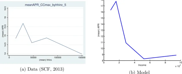
Also when analyzing realized interest rates relative to income, the model replicates important facts. Figure 2.2a depicts average loan prices in the data, measured by the APR, plotted against income quintiles. Low income households face much higher average cost, with a peak at the second quintile. When income increases, costs of credit decrease.
11For a theoretical derivation of increasing prices in the size of loans, see Chatterjee, Corbae, Nakajima,
and Ríos-Rull (2007, Theorem 6).
14 14.5 15 15.5 16 16.5 (mean) APR 0 50000 100000 150000 (mean) hhinc meanAPR_CCmax_byhhinc_5 (a) Data (SCF, 2013) 0 2 4 6 8 10 x 104 8 9 10 11 12 13 14 15 16 17 18 Income (mean) APR (b) Model
Figure 2.2: Average Credit Prices (APR), by income
Figure 2.2b depicts the model counterpart that exhibits the same features. Low income households tend to take smaller loans. Hence, fixed cost and higher nonpayment risk drive up prices for low income households.
The SCF oversamples high income households to precisely capture debt and asset holdings in the U.S. There is evidence that it does not contain complete information on the balance sheets of very low income households, though (Ratcliffe et al., 2007). The SCF recently introduced a question regarding the use of payday loans. When analyzing the balance sheet of households that report to use payday loans, these payday loans are rarely represented. Not being mentioned in the “other loans” category, small dollar loans are clearly underreported. Consequently, there are very few observations of very high interest rates in the SCF, even though small dollar loans are clearly used in reality.13
2.4 Delinquency as Insurance Device
This section highlights the trade-off of households that become delinquent or declare bankruptcy. Bankruptcy, on the one hand, might be prohibitively expensive in the period of filing for bankruptcy but offers total debt relief in the following period. If available, Chapter 7 bankruptcy thus insures households against adverse shocks. On the other hand, delinquency is more affordable in the short run (at least for low income households) but households enjoy no or only partial reduction of debt. I document that delinquent households might thus be “trapped” in debt long enough to repay more than they originally owed. Delinquency consequently provides low insurance or even anti-insurance. These findings will help to understand why the proposed repayment plan does not yield any
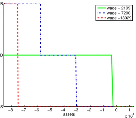
2.4 Delinquency as Insurance Device −8 −7 −6 −5 −4 −3 −2 −1 0 1 x 10⁴ S D B assets wage = 2199 wage = 7200 wage =13029
Figure 2.3: Repayment Decision, large expenditure shock
welfare gains (c.f. Section 2.5) whereas a bankruptcy advance makes households better off (c.f. Section 2.6).
2.4.1 Household Default Decisions
To understand the fundamental trade-off between delinquency and Chapter 7 bankruptcy, it is instructive to examine household default decisions more closely. Figure 2.3 depicts repayment decisions of low income, median income and high-income households that face a large expenditure shock. The policy functions p={S, D, B} are plotted as a function
of asset holdings minus the expenditure shock.14 High-income individuals can afford
repayment for very high levels of debt. Consequently, these individuals file for bankruptcy (p =B) only when debt is very high and otherwise stay solvent. Since they can easily
pay out-of-pocket expenses from current income, these households avoid delinquency and directly file for Chapter 7 bankruptcy.
Median income households cannot afford to repay such high levels of debt. Hence, they choose bankruptcy for lower levels of debt. Since out-of-pocket expenses of declaring bankruptcy are significant for these households, they choose delinquency (p= D) over
bankruptcy when debt is moderate. Only when debt levels are sufficiently high, these individuals choose bankruptcy in order to forgo collection efforts by banks.
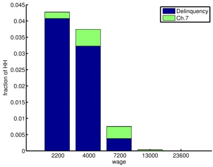
2200 4000 7200 13000 23600 0 0.005 0.01 0.015 0.02 0.025 0.03 0.035 0.04 0.045 wage fraction of HH Delinquency Ch.7
Figure 2.4: Average Repayment Decision
Low-income households, on the other hand, do not file for bankruptcy. When solvency becomes too expensive, these households become delinquent. Filing fees prove prohibitively high for these households, which de facto excludes them from Chapter 7 debt relief.15
The policy functions presented in Figure 2.3 clearly showed that low income households are effectively excluded from filing for Chapter 7 bankruptcy. This exclusion clearly materializes in the simulated equilibrium, too. Figure 2.4 presents repayment decisions as realized in equilibrium by income groups. Not surprisingly, higher income households are more likely to be solvent. While a significant fraction of low income households does not repay, they rarely file for Chapter 7 bankruptcy. Due to prohibitively high filing fees, these low income households rather become delinquent. As income increases, delinquency is substituted by filing for bankruptcy.
The cross-section of delinquency and bankruptcy filings with respect to income are not targeted in the calibration. The model nevertheless correctly predicts delinquencies to be more prevalent than bankruptcies for low income households. Table 2.4 compares the share of delinquencies and bankruptcy filings by households in the lowest 30% of the income distribution to the data. While fitting delinquencies quite well, the model underestimates bankruptcy filings by low income households.
15See Figure 2.B.1a in Appendix 2.B for the debt pricing function that results from this repayment
2.4 Delinquency as Insurance Device
Table 2.4: Non-Payment by 30% Lowest Income Households Non-Payment Decision Model Data
Delinquency 85% 75% Bankruptcy 42% 64%
Note: This table depicts the share of delinquency and bankruptcy decisions by households with the lowest 30% of income relative to total delinquency and bankruptcy decisions. Calculated from the Federal Reserve Bank of New York’s “Consumer Credit Panel / Equifax” data set (as seen in Athreya, Sánchez, Tam, and Young, 2015).
2.4.2 Delinquency as a “Debt Trap”
In the absence of state-contingent contracts, households use bankruptcy and delinquency to insure against adverse shocks. When choosing bankruptcy, households gain full debt relief in the next period. Debt relief tomorrow comes at a cost today: Bankrupts have to pay out-of-pocket fees F and they suffer utility cost ζB.
When choosing delinquency, households do not necessarily receive full debt relief in the next period. But, in the current period, cost of delinquency do not contain lump-sum expenditures. Delinquent households repay late feesL which depend on the household’s
state. Since banks make households indifferent between suffering collection or paying late fees, the total utility cost (relative to consuming the endowment) are simply the utility loss due to collection, ζD. Late fees can be directly backed out of the banks’ problem
in Equation (2.7). L = e −u−1(u(e)−ζ
D) makes the household indifferent between
consuminge−Lwithout utility cost or consuming e and facing a utility cost of ζD.
The difference in instantaneous utilities between delinquency and bankruptcy is ∆0 =u(e)−ζD −(u(e−F)−ζB) =U(e, F) +ζB−ζD, (2.10)
whereU(e, F) =u(e)−u(e−F) denotes the utility loss when paying lump sum filing fees F with income e. Hence, the difference in instantaneous utilities between delinquency and
bankruptcy (first term in Equation (2.10)) can be interpreted as the difference between the utility cost of bankruptcyU(e, F) +ζB and the utility cost of delinquency ζD (second
term in Equation (2.10)).
If ∆0 >0, delinquency is preferable relative to bankruptcy in the current period. In a
sense, it is a more affordable option to not repay outstanding debt. Thus, instantaneous utility from delinquency is higher than utility from bankruptcy, or equivalently, the utility cost of delinquency are lower than the cost of bankruptcy. Due to standard assumptions on the utility function (see the discussion following Equation (2.4)), utility cost of bankruptcy
0.4 0.6 0.8 1 1.2 1.4 1.6 1.8 x 10⁴ −15 −10 −5 0 5 10 15 Income ∆0 ∆ 1 ∆ 0+β∆1
Figure 2.5: Delinquency vs. Bankruptcy become infinitely large if filing cost F approach income:
U(e, F)→ ∞ for e−F →0, e > F.
If U(·) → ∞ , so does ∆0 → ∞. In other words, delinquency becomes increasingly
favorable as bankruptcy becomes infeasible (and instantaneous utility of bankruptcy diverges to −∞). In these cases, bankruptcy is not available for households to insure
against adverse shocks.16
In the period after delinquency or bankruptcy, expected values differ, too. While bankruptcy offers complete debt relief (a0 = 0), households in delinquency get partial or
no debt relief (a0 =α≤0). The difference between expected future utilities of delinquency
and bankruptcy thus is
∆1 =Es(V(α, s0)−V(0, s0)). (2.11)
Since V is a well-behaved value function, the expected future value of bankruptcy with
debt relief is higher than that of delinquency: −∞<∆1 ≤0. This is simply becauseV is
bounded and because ∂V /∂a >0.17
To sum up, households trade-off current period expenditures with future debt relief. Better insurance in bankruptcy (i.e. higher debt relief tomorrow) comes at higher cost
16On the other hand, ifF →0 ore→ ∞, lump sum fees become unimportant i.e. U(e, F)→0. Then,
the instantaneous utility difference converges to the difference in direct utility cost: ∆0→ζD−ζB. 17The last inequality can be strict, if∃α: q(α, s)α <0.