Multiclass and Multilabel
Classification
Vom Fachbereich Informatik der Technischen Universit¨at Darmstadt zur Erlangung des akademischen Grades eines
Doktor-Ingenieurs (Dr.-Ing.) genehmigte
Dissertation
vonDipl.-Inform. Sang-Hyeun Park (geboren in Frankfurt am Main)
Erstreferent: Prof. Dr. Johannes F¨urnkranz Korreferent: Prof. Dr. Eyke H¨ullermeier
(Philipps-Universit¨at Marburg) Tag der Einreichung: 29.03.12
Tag der Disputation: 24.05.12
D17 Darmstadt 2012
URL: http://tuprints.ulb.tu-darmstadt.de/2994
This document is provided by tuprints, E-Publishing-Service of the TU Darmstadt
http://tuprints.ulb.tu-darmstadt.de [email protected]
Decomposition-based methods are widely used for multiclass and multilabel classifi-cation. These approaches transform or reduce the original task to a set of smaller possibly simpler problems and allow thereby often to utilize many established learning algorithms, which are not amenable to the original task. Even for directly applicable learning algorithms, the combination with a decomposition-scheme may outperform the direct approach, e.g., if the resulting subproblems are simpler (in the sense of learnability). This thesis addresses mainly the efficiency of decomposition-based methods and provides several contributions improving the scalability with respect to the number of classes or labels, number of classifiers and number of instances.
Initially, we present two approaches improving the efficiency of the training phase of multiclass classification. The first of them shows that by minimizing redundant learning processes, which can occur in decomposition-based approaches for multiclass problems, the number of operations in the training phase can be significantly reduced. The second approach is tailored to Na¨ıve Bayes as base learner. By a tight coupling of Na¨ıve Bayes and arbitrary decompositions, it allows an even higher reduction of the training complexity with respect to the number of classifiers. Moreover, an approach improving the efficiency of the testing phase is also presented. It is capable of reducing testing effort with respect to the number of classes independently of the base learner.
Furthermore, efficient decomposition-based methods for multilabel classification are also addressed in this thesis. Besides proposing an efficient prediction method, an approach rebalancing predictive performance, time and memory complexity is presented. Aside from the efficiency-focused methods, this thesis contains also a study about a special case of the multilabel classification setting, which is elaborated, formalized and tackled by a prototypical decomposition-based approach.
Multiklassen- und Multilabel-Klassifikationsprobleme werden h¨aufig durch zerle-gungsbasierte Ans¨atze gel¨ost. Zerlegungsbasierte Ans¨atze haben gemeinsam, dass sie das urspr¨ungliche Problem auf eine Menge von kleineren potentiell einfacheren Problemen abbilden. Oft erm¨oglichen solche Ans¨atze die Wiederverwendung von vielen bew¨ahrten Lernalgorithmen, die nicht direkt auf das urspr¨ungliche Problem anwendbar sind. Dar¨uber hinaus k¨onnen auch f¨ur direkt anwendbare Lernalgorithmen die zerlegten Teilprobleme einfacher (im Sinne der Lernbarkeit) sein, so dass ein zerle-gungsbasierter Ansatz insgesamt eine h¨ohere Vorhersagequalit¨at besitzen kann als die direkte L¨osung des Problems. Diese Dissertation besch¨aftigt sich haupts¨achlich mit der Effizienz der zerlegungsbasierten Methoden und erarbeitet mehrere Ans¨atze mit einer besseren Skalierbarkeit bez¨uglich Anzahl der Klassen bzw. Labels, Klassifizierer und Instanzen der Daten.
Es werden zun¨achst zwei Ans¨atze vorgestellt, welche die Trainingsphase f¨ur Multi-klassenprobleme beschleunigen. In dem ersten Ansatz wird gezeigt, dass durch Mini-mierung von redundanten Lernvorg¨angen, die oft in zerlegungsbasierten Multiklassen-Klassifikationsans¨atzen vorkommen k¨onnen, Einsparungen in der Trainingsphase m¨oglich sind. Der zweite Ansatz ist speziell auf Na¨ıve Bayes als Basislerner ausge-richtet und erm¨oglicht durch die Ausnutzung spezieller Eigenschaften in diesem Fall eine noch gr¨oßere Reduktion der Lernkomplexit¨at bez¨uglich der Klassifiziereranzahl. Es wird zus¨atzlich ein Ansatz pr¨asentiert, welches die Klassifikationsphase f¨ur Mul-tiklassenprobleme beschleunigt. Dieses Verfahren ist unabh¨angig vom verwendeten Basislerner und reduziert die Klassifikationskomplexit¨at bez¨uglich der Klassenanzahl.
Dar¨uber hinaus werden in dieser Dissertation auch Multilabelprobleme behandelt und daf¨ur neben einer effizienten Klassifikationsmethode auch ein Ansatz vorgestellt, welches die Vorhersagequalit¨at, den Zeitaufwand und die Speicherkomplexit¨at neu abw¨agt. Neben den effizienzfokussierten Ans¨atzen beinhaltet diese Dissertation auch eine Studie, die einen Spezialfall von Multilabel-Klassifikationsproblemen vorstellt, formalisiert und mittels einem prototypischen zerlegungsbasierten Ansatz zu l¨osen versucht.
1 Introduction 1
1.1 Motivation . . . 2
1.2 Contributions. . . 2
1.3 Structure of this thesis. . . 3
2 Binary Classification 5 2.1 Binary Setting . . . 5
2.2 Classification Evaluation and Variants . . . 6
2.2.1 Standard Measures and Methods . . . 6
2.2.2 Cost-Sensitive Classification . . . 7
2.2.3 Area under the ROC Curve (AUC). . . 8
2.3 Learning Algorithms . . . 8
2.3.1 Rule Learning . . . 10
2.3.2 Decision Trees . . . 10
2.3.3 Perceptrons . . . 11
2.3.4 Support Vector Machines (SVM) . . . 12
2.3.5 Na¨ıve Bayes. . . 12
Part I Multiclass Classification 13 3 Multiclass Preliminaries 15 3.1 Multiclass Setting . . . 15
3.2 Multiclass Evaluation and Variants. . . 16
3.3 Common Decomposition-Based Approaches . . . 16
3.3.1 One-Against-All (OAA) . . . 16
3.3.2 Pairwise Classification (OAO) . . . 17
3.3.3 Efficient Pairwise Prediction (QWeighted) . . . 19
3.4 Error-Correcting Output Codes (ECOCs) . . . 21
3.4.1 Binary ECOCs . . . 21
3.4.2 Ternary ECOCs . . . 22
3.4.3 Code Design for (Ternary) ECOCs . . . 23
4 Efficient ECOC Training by Exploiting Code-Redundancies 27 4.1 Code Redundancy in ECOC . . . 27
4.2 Exploitation of Code Redundancies . . . 28
4.2.2 Greedy Computing of Steiner Trees . . . 32
4.2.3 Incremental Learning with Training Graph . . . 33
4.2.4 SVM Learning with Training Graph . . . 33
4.3 Experimental Evaluation . . . 35 4.3.1 Experimental Setup . . . 35 4.3.2 Hoeffding Trees. . . 36 4.3.3 LibSVM . . . 37 4.4 Related Work. . . 41 4.5 Conclusions . . . 41
5 Efficient ECOC Training with Na¨ıve Bayes 43 5.1 Na¨ıve Bayes. . . 44
5.2 Computation of ECOC for Na¨ıve Bayes in a single pass . . . 44
5.2.1 Reduction to Base Probabilities. . . 44
5.2.2 Complexity . . . 45 5.2.3 Precalculation . . . 46 5.2.4 ECOC-NBAlgorithm . . . 48 5.3 Experimental Evaluation . . . 48 5.3.1 Experimental Setup . . . 48 5.3.2 Accuracy Evaluation . . . 49 5.3.3 Run-time Evaluation. . . 50 5.4 Conclusions . . . 51
6 Efficient ECOC Prediction 55 6.1 Efficient ECOC Decoding . . . 55
6.1.1 Reducing Hamming Distances to Voting . . . 56
6.1.2 Next Classifier Selection . . . 57
6.1.3 Stopping Criterion . . . 57
6.1.4 Quick ECOC Algorithm . . . 58
6.1.5 Adaption to Different Decoding Strategies . . . 60
6.2 Experimental Evaluation . . . 63
6.2.1 Pairwise Classification - Evaluation of QWeighted . . . 63
6.2.2 ECOC Classification - Evaluation of QuickECOC. . . 70
6.3 Analysis of (k,3)-Exhaustive Ternary Codes . . . 78
6.4 Conclusions . . . 81
Part II Multilabel Classification 83 7 Multilabel Preliminaries 85 7.1 Multilabel Setting . . . 85
7.2 Multilabel Evaluation . . . 86
7.2.1 Labelset Loss Functions . . . 86
7.2.3 Averaging Methods . . . 90
7.3 Decomposition-Based Approaches . . . 90
7.3.1 Binary Relevance (BR) . . . 90
7.3.2 Multilabel Pairwise Learning (MLP) . . . 91
7.3.3 Calibrated Label Ranking (CLR) . . . 93
7.3.4 Hierarchy of Multilabel Classifiers (HOMER) . . . 94
8 Efficient Pairwise Multilabel Prediction 97 8.1 Perceptrons . . . 98
8.1.1 MLPP and CMLPP . . . 99
8.2 Quick Weighted Voting for Multilabel Classification . . . 99
8.2.1 QCMLPP1. . . 99 8.2.2 QCMLPP2. . . 101 8.2.3 Discussion. . . 101 8.3 Computational Complexity . . . 101 8.3.1 Memory Requirements . . . 101 8.3.2 Training . . . 102 8.3.3 Prediction . . . 102 8.4 Experimental Evaluation . . . 103 8.4.1 Datasets. . . 103 8.4.2 Experimental Setup . . . 105 8.4.3 Computational Efficiency . . . 105 8.4.4 Predictive Quality . . . 109
8.4.5 Support Vector Machines . . . 111
8.5 Conclusions . . . 112
9 Combination of Multilabel Classification Decompositions 115 9.1 Combination of HOMERand QCLR . . . 116
9.1.1 Memory-Complexity . . . 116
9.2 Experimental Evaluation . . . 117
9.2.1 Experimental Setup . . . 118
9.2.2 Results of HOMERwithQCLR. . . 118
9.2.3 Comparison of HOMERagainst its base classifiers. . . 124
9.3 Conclusions . . . 127
10 Multilabel Classification with Label Constraints 129 10.1 Label Constraints . . . 130
10.1.1 Definition of Label Constraints . . . 130
10.1.2 Constraint-Based Correction of Predictions . . . 131
10.1.3 Experimental Evaluation . . . 134
10.2 Discovering Label Constraints from Data . . . 136
10.2.1 Association Rules as Constraints . . . 137
10.2.2 Experiments on Real-World Data. . . 138
11 Summary 143 11.1 Summary . . . 143 11.2 Outlook . . . 145 Bibliography 149 Own Publications 159 A Appendix 163
3.1 One-against-all and pairwise binarization . . . 17
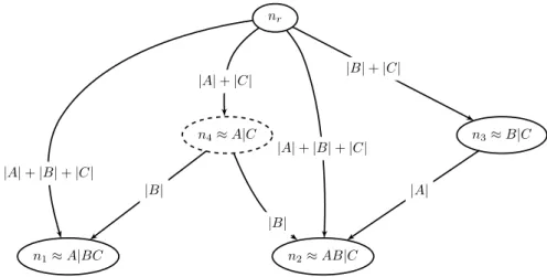
4.1 Training graph example . . . 29
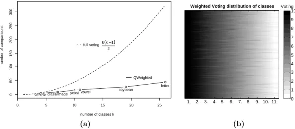
6.1 Prediction efficiency: QWeightedvs. full pairwise classifier. . . 66
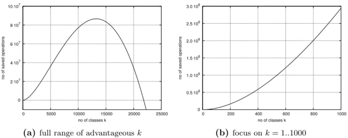
6.2 Approximate computational savings of QWeighted . . . 70
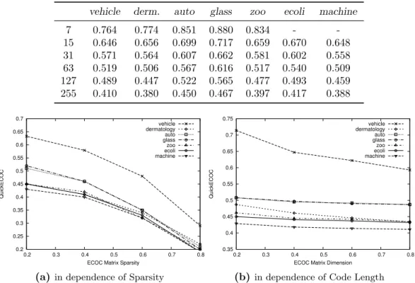
6.3 QuickECOCperformance on random codes . . . 73
6.4 QuickECOCanalysis: Dependency of stopping criteria (ecoli) . . . 79
6.5 QuickECOCanalysis: Impact of stopping criteria (ecoli) . . . 79
6.6 Simplified QuickECOCvs. actual performance (ecoli). . . 80
7.1 Diagrams of predicted label rankings . . . 89
7.2 Subproblems in binary relevance for multilabel classification . . . 91
7.3 Subproblems in pairwise multilabel classification . . . 91
7.4 MLP voting aggregation . . . 92
7.5 MLP training, calibration and CLR training . . . 93
7.6 CLR voting aggregation . . . 94
7.7 HOMER: Sample hierarchy multilabel classification task . . . 95
8.1 Prediction complexity of QWeightedand QCMLPP . . . 108
8.2 Prediction complexity of QCMLPP (more detailed) . . . 110
9.1 Micro recall over number of partitions for six HOMERvariants. . . 119
9.2 Micro precision over number of partitions for six HOMERvariants. 120 9.3 Micro F1 over number of partitions for sixHOMERvariants . . . . 121
9.4 Training time over number of partitions for six HOMERvariants. . 122
9.5 Testing time over number of partitions for six HOMERvariants . . 123
1 QWeighted . . . 20
2 Training Graph Generation . . . 31
3 Greedy Steiner Tree Computation . . . 32
4 ECOC-NB training scheme . . . 48
5 ECOC-NB testing scheme . . . 48
6 QuickECOC . . . 59
7 MLPP . . . 99
8 QCMLPP2 . . . 100
4.1 Training data reduction: standard vs. min-redundant scheme . . . . 37
4.2 Training runtime: standard vs. min-redundant scheme . . . 38
4.3 GSteiner running time in seconds . . . 38
4.4 Training time in seconds (cache size: 25 %). . . 39
4.5 GSteiner running time for random codes in seconds. . . 39
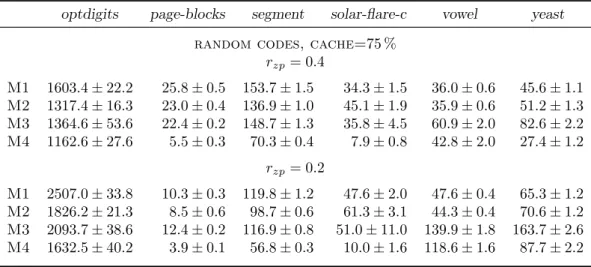
4.6 Training time in seconds of random codes (cache size: 75 %) . . . 40
4.7 Comparison of LibSVM optimization iterations. . . 40
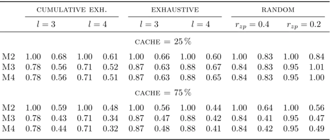
4.8 Cache efficiency and min-redundant training scheme impact . . . 41
5.1 ECOC-NB: Predictive performance (normal density estimators) . . 50
5.2 ECOC-NB: Predictive performance (kernel density estimators) . . . 51
5.3 ECOC-NB: Training efficiency (normal density estimators) . . . 52
5.4 ECOC-NB: Training efficiency (kernel density estimators). . . 53
5.5 Dataset characteristics . . . 54
6.1 Comparison of QWeightedand DDAG with various base learners . 65 6.2 Prediction complexity:QWeightedvs. full pairwise classifier . . . . 67
6.3 QWeightedperformance on datasets with high number of classes . 69 6.4 QuickECOCperformance on exhaustive ternary codes . . . 72
6.5 QuickECOCperformance on BCH Codes. . . 73
6.6 QuickECOCperformance with all decoding methods . . . 75
6.7 QuickECOCperformance on datasets with high number of classes. 76 6.8 Prediction complexity:QuickECOCvs. full ensemble of classifiers . 77 8.1 Computational complexity of BR,MLPPand QCMLPP . . . 102
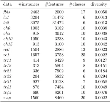
8.2 Dataset characteristics . . . 103
8.3 Computational prediction costs . . . 106
8.4 Predictive performance: BRvs.(Q)CMLPP . . . 109
8.5 Computational prediction costs (base learner: SVM) . . . 111
8.6 Predictive performance: BRvs.(Q)CMLPP(base learner: SVM) . 113 9.1 Dataset characteristics . . . 118
9.2 Performance of BR,QCLR,H+BRand H+QCLR . . . 125
9.3 Computational costs of BR,QCLR,H+BRand H+QCLR . . . . 126
10.1 Experiments on synthetic data generated with constraintsZ1 . . . . 135
10.3 Experiments on 100 random synthetic datasets . . . 136
10.4 Experiments on real-world data:yeast . . . 138
10.5 Experiments on real-world data:siam . . . 139
10.6 Constraint Generation:yeast . . . 140
10.7 Constraint Generation:siam. . . 140
A.1 Accuracy performance of ECOC with various code types . . . 163
A.2 ECOC Redundancies: results usingLibSVM (cum. exh. codes) . . . 164
A.3 ECOC Redundancies: results usingLibSVM (exh. codes) . . . 165
~
x, x∈X instance (see text), set of instances
t number of instances
D dataset
a∈A feature, set of features
g number of features
c∈K class, set of classes
λ∈L label, set of labels
k number of classes/labels
P relevant labels or positive classes
N irrelevant labels or negative classes
d average number of relevant labels
y output variable
f(x)∈C classifier, set of classifiers
n number of classifiers
~
cw= (b1, . . . , bn) code word, code bits
~
w weight vector
rzp random zero probability (random codes)
τ, τ(λ) ranking (of labels/classes), rank position of labelλ β number of partitions (HOMER)
z∈Z label constraint, set of label constraints
pr∈P R preference, set of preferences
q number of label constraints
N,R natural numbers, real numbers
S permutation space
The classification task is one of the most elementary problems in machine learning. The automatic learning of a predictor function from a given set oftraininginstances, which maps unseentest instances to its corresponding true class was studied exten-sively since the beginning of machine learning. The distinct formulation and easy comprehensibility of the underlying setting have certainly contributed to this high attention. It is a testbed from which many successful learning algorithms evolved, e.g.,Ripper/Slipper(Cohen,1995; Cohen and Singer,1999),C4.5 (Quinlan,1993) andSVM(Vapnik,1998).
It is apparent that automatic classification also has a high direct practical value. The possibility to learn an accurate predictor in domains such as speech recognition, optical character recognition or spam classification improves the convenience for humans. Though these tasks are in principle trivial for humans, in light of the increasing mass of digital information, manual classification becomes infeasible for large scale datasets and efficient automatic classification methods grow in importance. Another aspect is the automatic analysis of data, which may complement the human analysis and provide analternativeview – the rules of a learned classifier may expose previously unknown insights about the data. The aspired discovery of these so-called “nuggets”, i.e. new patterns or rules inherent in data, provides a strong incentive for
research in machine learning or data mining in general respectively.
Multiclass and multilabel classification are special cases of the above-mentioned classification task and impose different restrictions on the target output variable. For multiclass classification the target variable has to be one of a given set of identifiers, calledclasses. An example is the task of optical character recognition, where the target variable is one of the alphabetic or numeric characters. For the multilabel case, the target variable is a subset of a given set of classes. This means more than one class (in this context typically called labels) can be associated with the instance. A Germanmovie mcategorized as an action-film withcomedy-elements may be seen as
the multilabel instance (m,{german,comedy,action}).
These tasks are commonly tackled by so-calleddecomposition-basedapproaches, which transform the problem into a set of smaller possibly simpler problems. For instance, ak-class classification problem can be transformed to a set of binary (2-class) problems. This makes many classification algorithms which are only applicable for 2-class problems amenable for this task. Decompositions allow to reuse learn algorithms readily in more complex tasks by applying an appropriate transformation scheme. Besides this practical convenience, the decompositions to simpler problems can also lead to a better predictive and efficiency performance compared to the direct approach (Ghani,2000;Hsu and Lin,2002;F¨urnkranz,2002).
1.1 Motivation
In contrast to classical computer science algorithms such as sorting algorithms, where the only acceptable correctness is fully sortedand algorithm research was focused in minimizing time and memory complexity, in machine learning a perfect (predictive) result is seldom feasible. It is apparent to prioritize the predictive performance over time and memory complexity. Thus, predictive performance is the predominant measure considered in multiclass and multilabel methods.
However, in light of the growing amount of data which needs to be processed, the time and memory complexity increased in its importance. At the latest, in extreme cases, where the memory or time complexity presents an infeasible bottleneck for the whole task, a reprioritization of these factors is necessary.
Furthermore, as previously described, classification is one of the basic components, which is often employed in a modular way for more complex machine learning tasks. For example, throughout this thesis, multiclass and multilabel classification will be tackled by anensembleof binary classifiers. In general for multiclass classification, we will be concerned with so-callederror-correcting output codes (ECOC) which provide a unified framework for common decomposition-based ensemble types. Efficiency bottlenecks of base classifiers can drastically accumulate throughout the ensemble or the whole framework. This means also that efficiency improvements on the base classifier level may have a drastic overall reduction to the whole task.
Besides the illustrated extreme case, improving the efficiency can also implicitly improve the predictive performance. The sheer capability of processing more data in a fixed time means obviously to increase thesample-size and, therefore, to strengthen the statistical powerof the underlying statistical learning algorithms or at least of the various employed statistical measures.
1.2 Contributions
In this thesis, we present mainly efficiency and partly efficacy improvements for decomposition-based multiclass and multilabel classification methods.
Multiclass Classification
Efficient ECOC Training by Exploiting Code-Redundancies
ECOC-based classifier ensembles can have overlapping training processes. We develop a training schedule, which tries to minimize these redundant learning processes. This schedule based learning is directly applicable for genuine incremental learners, but we also develop modifications for the genuine batch learner SVMto be applicable for this approach.
Efficient ECOC Training with Na¨ıve Bayes
A simple tight combination of Na¨ıve Bayes and ECOC is presented, which reduces the training effort significantly compared to the straight-forward combination. This is mainly done by an alternative equivalent computation scheme exploiting some special relations in this setting.
Efficient ECOC Prediction
Here, we present an efficient prediction/decoding scheme for ECOC classifiers. It is based on the fact, that it is not always necessary to consider all classifier evaluations for the decoding phase. Although we do not give a theoretical average-case analysis, extensive empirical evaluations indicate the significance of this approach in practice.
Multilabel Classification
Efficient Pairwise Multilabel Prediction
Two efficient prediction algorithms for the calibrated label ranking approach for multilabel classification are presented. The prediction phase of the underlying ensemble of pairwise classifiers (special type of binary classifiers) is similarly improved as for the case of ECOC classifiers in multiclass prediction.
Combination of Multilabel Classification Decompositions
Here, the efficiency and also the predictive performance of the above approach is further improved in combination with theHOMERapproach, which transforms the original multilabel problem into a set of smaller multilabel problems. Multilabel Classification with Label Constraints
We consider a variant of the multilabel setting and elaborate on the existence of constraints, or at least, dependencies among labels in real data. Besides using association-rule learning to find such constraints, we experiment with two methods on incorporating them into the learning process.
1.3 Structure of this thesis
This thesis is divided into two parts:Part I is dedicated to multiclass andPart II to multilabel classification. Each part begins with its own preliminaries chapter (Chapter 3 and Chapter 7), which briefly recapitulates the setting, measures and common decomposition-based methods. Except for the introduction (Chapter 1), the introductory chapter on binary classification (Chapter 2) and the summary (Chapter 11), each of the remaining chapters is dedicated to one contribution, which in turn is based on a publication. The corresponding references are shown in the following list. Please note, that the basics chapters are also mainly based on these publications.
Part IMulticlass Classification
Chapter 4, Efficient ECOC Training by Exploiting Code-Redundancies (Park, Weizs¨acker, and F¨urnkranz,2010)
Chapter 5, Efficient ECOC Training with Na¨ıve Bayes (Park and F¨urnkranz,2011)
Chapter 6, Efficient ECOC Prediction (Park and F¨urnkranz,2012)
Part II Multilabel Classification
Chapter 8, Efficient Pairwise Multilabel Prediction (Loza Menc´ıa, Park, and F¨urnkranz,2010)
Chapter 9, Combination of Multilabel Classification Decompositions
(Tsoumakas, Loza Menc´ıa, Katakis, Park, and F¨urnkranz,2009) Chapter 10, Multilabel Classification with Label Constraints
Contents
2.1 Binary Setting . . . 5 2.2 Classification Evaluation and Variants . . . 6 2.2.1 Standard Measures and Methods . . . 6 2.2.2 Cost-Sensitive Classification . . . 7 2.2.3 Area under the ROC Curve (AUC) . . . 8 2.3 Learning Algorithms . . . 8 2.3.1 Rule Learning. . . 10 2.3.2 Decision Trees . . . 10 2.3.3 Perceptrons . . . 11 2.3.4 Support Vector Machines (SVM) . . . 12 2.3.5 Na¨ıve Bayes . . . 12
Binary classification refers to the task of automatically mapping input instances to their most probable class or category, where the number of classes is restricted to two classes. A multitude of approaches based on different learningconceptsoriginated for thesebinary problems.
This chapter contains a brief recapitulation of basic knowledge about binary classification and standard learning algorithms for this task.
2.1 Binary Setting
In the binary classification setting, we consider a set of instances/examples X =
{~xi |i= 1. . . t}, where each instance is associated to one of two classes. One often
speaks of thepositiveand thenegativeclass in this context, similarly also for instances, i.e. positive instances are instances which true class is the positive class and vice versa. Thus, we consider instance-class pairs (~x, y), wherey ∈ K = {cpos, cneg} or
{+,−}. Furthermore, each instance is represented as a vector~x= (a1, . . . , ag) in a
feature spaceRg.
Typically, a subset of instances ¯X ⊆X along with their corresponding true class associations is given, i.e. we have given a set of pairs (~x, y)i, which are used to learn
a classifierf(.) :X →K. This classifier is supposed to predict for previously unseen instances~xithe correct class, such that some performance criterion (e.g., classification
In the following, we will often neglect the vector notation of instances for convenience reasons, i.e. we will usexsynonymously with~x, except for cases, where we particularly focus on the featuresai of an instance. Furthermore, if it is clear from the context,
that the same instancexi is addressed, we will often also omit the index.
2.2 Classification Evaluation and Variants
2.2.1 Standard Measures and MethodsWe will provide a short description of standard performance measures and methods used in binary classification.
Accuracy
The following measure describes the empirical accuracyof classifierf for a given set of instances ¯X, which is the predominant predictive evaluation measure in binary classification. Acc(f,X¯) := 1 t t X i=1 I(f(xi) =yi)
whereI(.) denotes the indicator function, which returns 1 if the statement is true and 0 otherwise. It represents the fraction of correctly predicted instances. Usually, one is interested in obtaining a classifier, which optimizes this measure for unseen related instances. This task is typically viewed in the following way: the given (training-) set of instances ¯X represents onlya subset of an unknown complete, possibly infinite set of instancesX and we are rather interested in a classifier which optimizesAcc(f, X). Thus, instances x∈X, which are not necessarily members of ¯X can appear during the prediction phase. In probabilistic terms, the general objective is to maximize
E(x,y)∼XI(f(x) =y)
The expected value of the complementary event, i.e. I(f(x)6=y), is also called the true riskof a classifierf.
True Negative Rate and True Positive Rate
The true negative rate (TNR) and true positive rate (TPR) describe the accuracy only for one of the two classes, i.e. it describes the fraction of correctly predicted negative or positive instances respectively. The computation is similar to accuracy except that one iterates only over the negative or positive instances respectively. False Negative Rate and False Positive Rate
The false negative rate (FNR) describes the fraction of positive instances which were incorrectly classified as negative ones, or shorter, the fraction of incorrectly predicted
positive instances. This equals 1−TPR or can be computed similarly as the TPR by considering only positive instances and determining the fraction of mispredictions, i.e.I(f(xi)6=yi).
Similar to the false negative rate, the false positive rate (TPR) describes the ratio of incorrectly predicted negative instances, i.e. which were predicted as positive. Again, it can be computed by 1−TNR or if TNR is not given in a straight-forward manner.
Cross-Validation
Since, in practice, the complete set of instances is not known or not finite, one can only approximate the true risk or other similar measures of a classifier. One well-known approach for evaluating thegeneralizationproperty of a classifier iscross-validation. This method repeatedly trains and tests on disjoint subsets of the given data such that each instance serves at least once as training instance as well as testing instance. First, the dataset is equally divided intonfolds. Then, the classifier is typically evaluated by using n−1 folds for training and the remaining fold for testing. This process is repeated n-times, such that each fold is used exactly once for testing. Finally, the multiple evaluation results are combined by averaging. This process is called
n-fold cross validation and if the folds are additionally sampled according to the class distribution of the set of training instances, one speaks ofstratified cross-validation. Furthermore, the special case ofn=t, i.e. considering each single instance as a fold, is calledleave-one-out validation.
2.2.2 Cost-Sensitive Classification
Cost-sensitive classification is a variant of the basic setting. Until now, accuracy treated each class as equally important. This is sometimes not the case in real-world problems. For instance, the prediction of not cancer of a patient, who has cancer is obviously a more severe error than the reverse case. So, in this setting different importance among classes and the severity of their mispredictions are tackled by associating different cost-valuesγa,bfor each pair of classes (true classaand predicted
classb). Thus, the objective in this case is to minimize acost-weightederror measure:
Cost(f,X¯) = 1 t t X i=1 I( ˆyi 6=yi)·γyi,yˆi where ˆyi =f(xi)
For the multiclass classification setting, which will be introduced in the next chapter and involves more than two classes, the cost matrix γa,b ∈ RK×K allows not only
to associate different cost values for the mispredictionbetween classes, e.g., that a misprediction of the diagnosisnot canceris more costly than the misprediction of cancer. It is also possible to differentiate between different mispredictions for each class, for instance in weather forecasting (posed as a 3-class problem) that for the true eventhot, the misprediction of coldis associated with a higher cost than mild.
Note that the cost-sensitive classification setting is actually a generalization of the standard classification setting. By setting all elements of the cost matrix to 1, the objective is reduced to accuracy. Actually, it is sufficient when the non-diagonal elements are set to 1. Here, the diagonal elements are essentially ignored, since the indicator function returns in these cases (correct predictions) a value of zero.
2.2.3 Area under the ROC Curve (AUC)
Besides accuracy and cost-weighted errors, in some related tasks, one is interested in the ranking capability of classifiers. Here, classifiers are assumed to return ascore
s∈Rwhich quantifies the degree of class-membership of an instance. Classification
can be achieved by using an appropriate thresholding value, which divides the space of score values into positive and negative class spaces (in the two-class case). To assess such ranking capabilities of a classifier/rankerf thearea under the ROC curve(AUC) is commonly used. The receiver operating characteristic (ROC) curve has its origin from signal theory and was adapted to the machine learning field. Foremost, it is a graphical 2-d plot, which shows the false positive rate (x-axis) and the true positive rate (y-axis) of a binary classifier for varying thresholding values. If the classifier f is a good ranker, i.e. if positive examples are mostly ranked before negative examples with respect to their score, the ROC curve should ideally be convex, lie clearly above the diagonal (which represents a random ranker) and close as possible to the axis parallels of the unit square. The area under the ROC curve, i.e. the integral of the ROC curve, summarizes these criteria roughly in a single value.
2.3 Learning Algorithms
Before we provide superficial descriptions of some common learning algorithms, we will recapitulate in the following text a brief general view of learning algorithms based on (Mitchell,1997;Witten et al.,2011).
It is not an easy task to give a general unified view over the multitude of various learning algorithms for classification. Some textbooks regard the learning process as a search process to provide a simple unified view for introductory purposes. A large portion of learning algorithms are covered by this perspective (but not all), particularly if one considers that optimization problems can be viewed as a search problem similarly. So, we make use of the same perspective here. Assuming an enumerable space of all learnable classifier functions (e.g., linear or axis-parallel decision boundaries in the feature space) for a given learning algorithm, the task is to find a classifier function which maximizes some criterion on the training data. A simple algorithm which enumerates over all possible classifier functions and determines thereby the maximizer might represent a sufficient learning algorithm, if the search space is finite and small enough. But, this is seldom the case, such that typical learning algorithms employ different more efficient but also not necessarily globally optimal methods to be practical.
One important concept related to the generalization property of classifiers is the inductive bias, which consists of a set of assumptions or restrictions related to the learning process. To generalize, we have to make some assumptions about the classifier function and the data. Amongst others, we have to precisely definein which form we generalize. An overly simplified but illustrative example which is often used for describing inductive reasoning is the following:
Socrates is a human. Socrates is mortal.
o Induction
−−−−−−→ All humans are mortal.
Now, there is no real justification for generalizing the mortal property toall humans. It is equally valid to infer that, e.g., 2 human beings are mortal or only the next encountered human is mortal. As one might have noticed, the generalization is obviously influenced by the choice ofoperatorsand/or quantifierswe allow and in general by thelanguage in which statements are formed.
The previous simple example shows that the form of generalization can differ, and that there is no general right choice. But it is clear that these kind of decisions have to be made eventually during learning. Another example is to fit a line to a set of observed 2-dimensional points. Here, we make the assumption that the x, y
coordinates have a linear relationship and have restricted the model to lines, excluding arbitrary functions. In general, we have no guarantee that the “true” relationship which generated these points might not have been a very spiky curve. Of course, by using the assumption that the examples are independent and identically distributed, we get a different situation. But, also here, in the extreme case, where we do not restrict the classifier function, we may end up with a function which represents the total memorization of the points, if we are primarily searching for a classifier function which matches the most with the training data. This kind of overly adapting the model to the training data and therefore losing its generalization capabilities is called overfitting. In total, it is essential to the learning process to impose some restrictions and make assumptions on the classifier function as well as on the data.
Consider the set of arbitrary classifier functions, then, different actual learning algorithms can be superficially characterized by imposing different explicit and implicit biases/restrictions distinguished in three categories:
• description language or model: What is the underlying representation language used by the classifier? For rule learning, it might be arbitrary proposi-tional logic formulas. For perceptrons, the search space consists of all possible hyperplanes of the feature space.
• search-method, optimization and details: In which order, if any, is the search space examined. Is a greedy method, e.g. gradient descent, applied? Which additional criteria are used during search?
• overfitting-avoidance method: Are there separate mechanics for this pur-pose? In which form are they integrated?
In the following, we will provide only a brief overview of some common learning algorithms in its most basic form. Detailed knowledge about these algorithms are in general not necessary for this thesis, since the contributions in the following chapters are mostly independent of the used base learner. However, if the details of a particular learning algorithm are relevant, a more detailed description will be provided in the corresponding chapter (SVMs inChapter 4, Na¨ıve Bayes inChapter 5 and perceptrons in Chapter 8).
2.3.1 Rule Learning
In this context, the objective is to learn a set of rules in the following form: IF attribute-value condition(s) THEN class y
The conditions which are formed by conjunctions of propositions using the given fea-ture representation are typically learned within the separate-and-conquerframework. Starting from the empty rule, i.e. the set of attribute-value conditions is empty, one tries to determine the best attribute-test according to some measure on the resulting partitioning and is added to the set of conditions. This process is repeated until some stopping criterion is met. Then, the implication of the rule is associated with the majority class of the covered instances, i.e. the instances which satisfy the conditions. Afterwards, all instances which are covered by this rule are removed from the training set (SEPARATE). The process repeats by learning the next rule (CONQUER), until, again, some stopping criteria is met. Some rule learning algorithms try to learn only rules for one class and conclude the set of rules with a so-called default-rule, which classifies all remaining instances with the other class.
Within this thesis, our choice of a rule learner in various experiments is Ripper (Cohen,1995) in its implementation of the Weka-framework (Hall et al.,2009), called
JRip.
2.3.2 Decision Trees
The generation of decision trees can be viewed as a learning process, which generates non-overlapping rules arranged in a tree. Starting with all training instances, an attribute is determined according to some criterion which generates a partitioning of the training data corresponding to the values of this attribute. The attribute is represented as a node in a graph, from which directed edges are connected to child nodes, one for each different attribute value. These child nodes represent the partitions, which satisfy the corresponding attribute-value test. This process is recursively repeated on the child nodes until all remaining instances are members of one class or met some stopping criterion. Now, if you consider each path from the root node to the leaf, it represents a rule consisting of the conjunction of attribute-value tests and an implication to a particular class. The non-overlapping property follows by considering that for each pair of distinct root-leaf paths, there is exactly one attribute-test, in which they exclude each other. This kind of recursive explicit
excluding process is commonly referred to as thedivide-and-conquer approach in contrast to the separate-and-conquer approach from rule learning, where different rules can cover the same instance.
The above-mentioned criteria to select the next attribute is typically minimizing the spreadof instances of each class to different partitions. Examples of measures which address this issue are Information Gain and the Gini-Index (Breiman et al.,1984). In the following chapters, we will mainly use the implementation of C4.5 (Quinlan, 1993) in Weka (Hall et al.,2009), calledJ48, as a representative for decision tree learners.
Hoeffding Trees
Hoeffding Trees (Domingos and Hulten,2000) are a special kind of decision trees, which make use of the so-called Hoeffding-bound. It is a result known from statistics, which provides an upper bound on the probability, that the empirical mean of random variables deviates from its expected value by some value t. Consider the previously mentioned attribute-selection criterion for decision trees evaluating each attribute by a numeric valuevc in an incremental manner. Using the bound it is possible to
make the statement after observing a portion of the instances, that the current best attribute is with a specifiable probability really the best attribute, if the mean of its corresponding valuevbest has a larger distance to the mean of the second best attribute valuevsecond thant. Roughly speaking, the mean of the random variable
vbest stabilizeswith increasing number of observations. The Hoeffding bound allows to compute the number of necessary observations or instances, after which it is very unlikely that the deviation is higher than the distance to the second best attribute value. So, it is possible to select attributes and therefore build a decision tree in an incremental manner instead after observing all instances. In total, this results in a very fast incremental decision tree learner with anytime properties, i.e. it is possible to classify during the learning process. One of its main features is that its prediction is guaranteed to be asymptotically nearly identical to that of a corresponding batch learned tree.
2.3.3 Perceptrons
Perceptrons or artificial neurons (McCulloch and Pitts,1943;Rosenblatt,1958) are based on the human neurons in the brain. Human neurons are inter-connected and influence each other. Theactivationorexcitationof a neuron, which can be caused for instance by seeing something, is distributed in different strengths among its connected neurons, where each neuron may react differently to the input signals. The actual functionality of a neuron is modeled in perceptrons as a simple linear combination of its input signals accompanied with a thresholding function. The weighted sum of the input signals have to satisfy some threshold to forward an activation signal and the learning task is essentially to learn the weights.
For the learning of complex functions, typically a network of artificial neurons are utilized, which are calledartificial neural networks. However, a single artificial neuron is also often used as a classifier model, i.e. a linear function is learned which (by thresholding) discriminates one class against another one, often visualized as a hyperplane of the feature/input space, which separates instances of different classes. 2.3.4 Support Vector Machines (SVM)
Roughly speaking, support vector machines (Vapnik,1998) also learn a linear separator but include two significant techniques. First, it is possible to alter the working feature space in an efficient way by using so-calledkernel functions, i.e. it is possible to learn a linear separating function in some projected feature space in feasible time. Since it is nearly always possible to learn a linear separable function in a sufficient high-dimensional feature space for a given set of training instances, this technique makes a powerful tool. However, because of the resulting massive flexibility of the model, the probability of overfitting increases. One integral approach of SVMs which tries to address this issue, is to select the one separator from the possibly infinite set of linear separators, which maximizes the margin, i.e. the distance between the hyperplane to the nearest positive example plus the distance from it to the nearest negative example. This margin-maximization principle has to be shown to have desireable properties with respect to generalization (Shawe-Taylor et al.,1998;Smola et al.,2000).
In this thesis, we will utilize three different implementations/variants of SVMs: an SVM implementation in Weka called SMO, the implementation of LibLinear (Fan et al.,2008) and the one from LibSVM (Chang and Lin,2011).
2.3.5 Na¨ıve Bayes
Na¨ıve Bayes is one of the probabilistic approaches to classification. It is assumed, that there exists a joint probability distribution of instance-class pair events and the classification objective is to return the most probable class, after observing a test instance. Thus, basically, the learning of such a model is primarily focused with estimating relevant probabilities from training data. Since the estimation of the prob-ability distribution requires a very large number of instances, the direct approach is in general not practical. Na¨ıve Bayes makes a probabilistic model amenable by imposing a strong assumption about the distribution. It uses a “naive” assumption, namely that the attributes are conditionally independent given the class. In combination with the Bayes Theorem, this makes the training process tremendously efficient and feasible.
Again, we used in this thesis the Na¨ıve Bayes implementation of Weka, denoted by NB.
Multiclass Classification
3 Multiclass Preliminaries 15
4 Efficient ECOC Training by Exploiting Code-Redundancies 27
5 Efficient ECOC Training with Na¨ıve Bayes 43
Contents
3.1 Multiclass Setting . . . 15 3.2 Multiclass Evaluation and Variants . . . 16 3.3 Common Decomposition-Based Approaches . . . 16 3.3.1 One-Against-All (OAA) . . . 16
3.3.2 Pairwise Classification (OAO) . . . 17
3.3.3 Efficient Pairwise Prediction (QWeighted). . . 19
3.4 Error-Correcting Output Codes (ECOCs) . . . 21 3.4.1 Binary ECOCs . . . 21 3.4.2 Ternary ECOCs . . . 22 3.4.3 Code Design for (Ternary) ECOCs . . . 23
Multiclass classification extends binary classification by considering more than two classes. For multiclass classification problems, besides direct multiclass-capable learn-ing algorithms, the common approaches are so-called decomposition-based approaches, which reuse binary learners from the previous chapter.
This chapter contains a brief recapitulation of basic knowledge about multiclass clas-sification and decomposition-based approaches for this task. We will focus particularly only on necessary information for this thesis.
3.1 Multiclass Setting
The multiclass classification setting is identical to the binary classification setting except that now the set of classesK = {ci |i= 1. . . k} is not anymore restricted
to two classes, i.e. k ≥ 2 instead of k = 2. It is assumed, that there exists at least one instance for each class. Moreover, the number of instances t is typically significantly greater than the number of classesk in order to make any reasonable induction.
One typical example of multiclass classification problems is optical character recog-nition. Here, the task is to recover a text, which is given in an image-representation. Seen as a classification task, a natural approach is to consider each alphabetic and numeric character as a class. This task becomes non-trivial for hand-written texts and also for machine-generated texts, e.g., by considering the multitude of different font styles.
3.2 Multiclass Evaluation and Variants
Nearly all previously introduced measures and setting variants for binary classification apply straight-forwardly also for multiclass classification. We will briefly describe the few exceptions in the following text.
The previously introduced measures true positive rate and true negative rate, which were essentially class-based accuracy values apply also for the multiclass setting. However, there is no more the distinction betweenthepositive andthenegative class, such that both notions lose the association to a particular class. The underlying semantic becomes essentially redundant if we neglect this. Thus, often only one term, the true positive rate regardinga particular class ca is used to denote the class-based
accuracy ofca.
Similarly, the semantics of the notions of false negative and false positive rates have to be slightly altered. Again, the semantic for both notions changes. Not the misprediction rate of positive or negative instances are determined respectively, but all mispredictions predicting a particular class. Here also, one usually agrees on one term, the false positive rate regarding a particular class, to denote the measure in this sense.
Regarding the AUC, there is no consensus for the multiclass case, but various approaches which tackle the multiclass ROC analysis by projecting them to binary ones were proposed in the literature (Hand and Till,2001;Provost and Domingos, 2003).
3.3 Common Decomposition-Based Approaches
Many learning algorithms can only deal with two-class problems. For multiclass problems, they have to rely onbinary decomposition(orbinarization)procedures that transform the original learning problem into a series of binary learning problems. In the following, we will recapitulate the well-knownone-against-allandone-against-one decompositions, which will be used throughout this thesis. Afterwards, in the next section, we will describe a general framework for decomposition-based approaches. 3.3.1 One-Against-All (OAA)
A standard solution for this problem is the one-against-all approach, also known as one-against-rest, which constructs one binary classifierfi for each class ci, where the
positive training examples are those belonging to this class and the negative training examples are formed by the union of all other classes, i.e. all remaining examples. An illustration of this decomposition scheme is shown inFigure 3.1aon the facing page.
At prediction time, all classifiers are queried on the given test instance. If exactly one classifierfipredicts the instance as positive, the corresponding classciis returned
as the overall prediction. For the other cases, i.e., if more than one or none classifier predicts the instance as positive, usually two solutions are possible. If the classifiers return score, confidence or probability values instead of a binary value (negative or
~ ~ ~ ~ ~ ~ ~ ~ ~ ~ ~ ~ ~ ~ -- -- -- -# # # # # # # # # # # # o o o o o o o o o o o o o o o o o o o + + ++ + + + + + + + + + + + + + + x x x x x x x x x x x x x x
(a)One-Against-All Classification:
kclassifiers, each separates one class from all other classes. Here:+against all other classes
~ ~ ~ ~ ~ ~ ~ ~ ~ ~ ~ ~ ~ ~ + + ++ + + + + + + + + + + + + + + (b) Pairwise Classification: k(k−1)
2 classifiers, one for each pair of classes.
Here: + against∼.
Figure 3.1: One-against-all and pairwise binarization (F¨urnkranz, 2002)
positive), one can return the class, which corresponding classifier maximizes this measure. In the case, that the maximal value is not unique, or the classifiers return only binary values, one usually applies a random tie-breaking, i.e. randomly selecting one class among the set of predicted classes.
3.3.2 Pairwise Classification (OAO)
Pairwise classification also known as round-robin classification (F¨urnkranz, 2002; Wu et al., 2004) and one-against-oneis besides one-against-all one of the well-known decomposition schemes. This approach has been shown to produce more accurate results than the one-against-all approach for a wide variety of learning algorithms such as support vector machines (Hsu and Lin, 2002) or rule learning algorithms (F¨urnkranz,2002). Further support is given by a recent extensive experimental study
ofGalar et al. (2011).
The key idea of pairwise classification is to learn one classifier for each pair of classes. At classification time, the prediction of these classifiers are then combined into an overall prediction.
Training Phase
A pairwise or round robin classifier trains a set ofk(k−1)/2 binary classifiers fi,j,
one for each pair of classes (ci, cj), i < j. Each binary classifier is only trained on
the subset of training examples belonging to classesci and cj, all other examples are
ignored1 for the training offi,j. An example of this procedure is shown inFigure 3.1b.
1 Several extensions of the pairwise approach, such as Tri-Class SVMs (Angulo et al.,2006) and Pairwise Correcting Classifiers (Moreira and Mayoraz,1998), also integrate the remaining examples
We will refer to the learning algorithm that is used to train these classifiers fi,j as
thebase learner. We will also say that classifierfi,j is incident to classesci andcj.
It is important to note that the total effort required to train the entire ensemble of thek(k−1)/2 classifiers is only linear in the number of classesk, and, in fact, cheaper than the training of a one-against-all ensemble. It is easy to see this, if one considers that in the one-against-all case each training example is used k times (namely in each of the k binary problems), while in the round robin approach each example is only used k−1 times, namely only in those binary problems, where its own class is paired against one of the otherk−1 classes (cf. alsoF¨urnkranz,2002).
Typically, the binary classifiers are class-symmetric, i.e., the classifiersfi,j and fj,i
are identical. However, for some types of classifiers this does not hold. For example, standard rule learning algorithms will always learn rules for the positive class, and classify all uncovered examples as negative. Thus, the predictions may depend on whether class ci or class cj has been used as the positive class. As has been noted
in (F¨urnkranz,2002), a simple method for solving this problem is to average the predictions of fi,j and fj,i, which basically amounts to the use of a so-calleddouble
round robin procedure, where we have two classifiers for each pair of classes. Prediction Phase
At classification time, each binary classifier fi,j is queried and issues a vote (a
prediction for either ci or cj) for the given example. This can be compared with
sports and games tournaments, in which each player plays each other player once. In each game, the winner receives a point, and the player with the maximum number of points is the winner of the tournament.
In this thesis, we will assume binary classifiers fi,j that return class probabilities
p(ci|ci∨cj) andp(cj |ci∨cj) if not stated otherwise. These can be used forweighted
voting (also called max-wins), i.e., we predict the classc∗ that receives the maximum weighted number of votes:
c∗ = argmax
c∈K
X
c0∈K\c
p c|c∨c0
Other choices for decoding pairwise classifiers are possible (cf., e.g., Wu et al., 2004; Hastie and Tibshirani, 1997), but voting is surprisingly stable. For example, one can show that weighted voting, where each binary vote is split according to the probability distribution estimated by the binary classifier, minimizes the Spearman’s rank correlation coefficient with the correct ranking of classes, provided that the classifier provides good probability estimates (H¨ullermeier et al.,2008). Also, empiri-cally and theoretiempiri-cally, weighted voting seems to be a fairly robust method that is hard to beat with other, more complex methods (H¨ullermeier and F¨urnkranz,2004; H¨ullermeier and Vanderlooy,2010).
into the training process. In several experiments, this has lead to an improved performance, which has to be paid with a considerable increase in training time, and more complex decision boundaries for the involved classifiers.
3.3.3 Efficient Pairwise Prediction (QWeighted)
Although the training effort for the entire ensemble of pairwise classifiers is only linear in the number of examples, at prediction time we still have to query a quadratic number of classifiers, which can be very inefficient for a high number of classesk. In this section, we discuss a recently proposed algorithm (Park, 2006; Park and F¨urnkranz, 2007) that allows to significantly reduce the number of classifier evaluations in practice without changing the prediction of the ensemble.
Key Idea
Weighted or unweighted voting predicts the top rank classc∗ by returning the class with the highest accumulated voting mass after evaluation of all pairwise classifiers. During such a procedure there exist many situations where particular classes can be excluded from the set of possible top rank classes, even if they reach the maximal voting mass in the remaining evaluations. Consider the following simple example: Givenk classes and an arbitrary numberj ∈Nwith j < k, if, currently, classcb has
lostj votings and classcahas received more than k−j votes, it is impossible for cb
to achieve a higher total voting mass thanca. Thus further evaluations involving cb
can be safely ignored for the comparison of these two classes.
To increase the reduction of evaluations we are interested in obtaining such exploitable situations frequently. Pairwise classifiers will be selected depending on a loss value, which is the amount of potential voting mass that a class hasnot received. More specifically, the lossli of a class ci is defined as li :=pi−vi, where pi is the
number of evaluated incident classifiers ofci and vi is the current vote amount ofci.
Obviously, the loss will begin with a value of zero and is monotonically increasing. The class with the current minimal loss is one of the top candidates for the top rank class.
The QWeighted Algorithm
Algorithm 1on the next page shows the QWeighted algorithm, which implements this idea. First, the pairwise classifierfa,b will be selected for which the lossesla and
lb of the relevant classesca and cb are minimal, provided that the classifierfa,b has
not yet been evaluated. In the case of multiple classes that have the same minimal loss, there exists no further distinction, and we select a class randomly from this set. Then, the lossesla andlb will be updated based on the evaluation returned byfa,b
(recall thatvab is interpreted as the amount of the voting mass of the classifierfa,b
that goes to classca and 1−vab is the amount that goes to classcb). These two steps
will be repeated until all classifiers for the classcm with the minimal loss has been
evaluated. Thus the current/estimated losslm is the correct loss for this class. As all
other classes already have a greater or equal loss and considering that the losses are monotonically increasing,cm is the correct top rank class or among the set of equal
Algorithm 1 QWeighted
Require: pairwise classifiers fi,j with 1≤i < j ≤k, testing instance x∈X
1: ~l∈Rk←0 # loss values vector
2: c∗ ←NULL
3: G← ∅ # keep track of evaluated classifiers
4: whilec∗= NULL do
5: ca←argmin ci∈K
li # select top candidate class
6: cb←argmin cj∈K\{ca},fa,j∈/G
lj # select second
7: if nocb existsthen
8: c∗ ←ca # top rank class determined
9: else # evaluate
10: vab←fa,b(x) # one vote for ca (vab = 1) orcb (vab= 0)
11: la←la+ (1−vab) # update voting loss forca
12: lb ←lb+vab # update voting loss forcb
13: G←G∪fa,b # update already evaluated classifiers
14: return c∗
Theoretically, a minimal number of comparisons of k−1 is possible (best case). Assuming that the incident classifiers of the correct top rank c∗ always return the maximum voting amount (l∗ = 0),c∗ is always in the set{cj ∈K |lj = minci∈Kli}. In addition, c∗ should be selected as the first class in step 1 of the algorithm among the classes with the minimal loss value. It follows that exactlyk−1 comparisons will be evaluated, more precisely all incident classifiers ofc∗. The algorithm terminates and returnsc∗ as the correct top rank.
The worst case, on the other hand, is still k(k−1)/2 comparisons, which can, e.g., occur if all pairwise classifiers classify randomly with a probability of 0.5. In practice, the number of comparisons will be somewhere between these two extremes, depending on the nature of the problem.
QWeightedwill always predict the same class as the full pairwise classifier except for ambiguous predictions, but the actual runtime complexity of the algorithm is close to linear in the number of classes, in particular for large numbers of classes, where the problem is most stringent. For very hard problems, where the performance of the binary classifiers reduces to random guessing, its worst-case performance is still quadratic in the number of classes as mentioned before, but even there practical gains can be expected. These properties of QWeighted are based on empirical evaluations done in (Park and F¨urnkranz,2007) and will be re-validated later in Section 6.2.1on page 63 on extended experiments.
Alternative Approaches
The lossli, which we use for selecting the next classifier, is essentially identical to the
allows to reliably conclude a class when not all of the pairwise classifiers are present. For example, Cutzu claims that using the voting-against rule one could correctly predict classci even if none of the incident pairwise classifiers fi,j (j= 1. . . k, j 6=i)
are used. However, this argument is based on the assumption that all base classifiers classify correctly. Moreover, if there is a second classcj that should ideally receive
k−2 votes, voting-against could only conclude a tie between classes ci and cj, as
long as the vote of classifierfi,j is not known. The main contribution of his work,
however, is a method for computing posterior class probabilities in the voting-against scenario.
The voting-against principle was already used byPlatt et al. (1999) earlier in the form of DDAGs (Decision Directed Acyclic Graphs), which organize the binary base classifiers in a decision graph. Each node represents a binary decision that rules out the class that is not predicted by the corresponding binary classifier. At classification time, only the classifiers on the path from the root to a leaf of the tree (at mostk−1 classifiers) are consulted. While the authors empirically show that the method does not lose accuracy on three benchmark problems, it does not have the guarantee of QWeighted, which will always predict the same class as the full pairwise classifier. Intuitively, one would also presume that a static evaluation routine that uses onlyk−1 of thek(k−1)/2 base classifiers will sacrifice one of the main strengths of the pairwise approach, namely that the influence of a single incorrectly trained binary classifier is diminished in a large ensemble of classifiers (F¨urnkranz,2003). Our empirical results (presented in Section 6.2.1on page 63) will confirm that DDAGs are only slightly
more efficient but less accurate than theQWeightedapproach.
3.4 Error-Correcting Output Codes (ECOCs)
Error-correcting output codes (ECOCs) (Dietterich and Bakiri,1995) are a general framework for decomposition-based multiclass classification methods. This frame-work unifies common approaches such as the previously described one-against-one and one-against-all. ECOCs have its origin in coding and Information Theory (MacWilliams and Sloane,1983;Gallager,1968), where it is used for detecting and correcting errors in suitably encoded signals. In the context of classification, we encode the class variable with an n-dimensional binary code word, whose entries specify whether the example in question is a positive or a negative example in the corresponding binary classifier.
3.4.1 Binary ECOCs
Formally, each class ci (i= 1. . . k) is associated with a so-calledcode word cw~ i ∈
{−1,1}n of lengthn. We denote thej-th bit ofcw~
i asbi,j. In the context of ECOC,
all relevant information is summarized in a so-calledcoding matrix (mi,j) =M ∈
{−1,1}k×n, whose i-th row describes code word cw~
i, whereas thej-th column
Furthermore, the coding matrix implicitly describes a decomposition scheme of the original multiclass problem. In each columnj the rows contain a (1) for all classes whose training examples are used as positive examples, and (−1) for all negative examples for the corresponding classifier fj.
M = 1 1 1 −1 −1 −1 1 −1 −1 1 1 −1 −1 −1 −1 1 −1 1 −1 −1 1 −1 1 1
The previous example shows a coding matrix for 4 classes (rows), which are encoded with 6 classifiers (columns). The first classifier uses the examples of classes 1 and 2 as positive examples, and the examples of classes 3 and 4 as negative examples.
At prediction time, all binary classifiers are queried, and collectively predict an n -dimensional vector, which must bedecoded into one of the original class values, e.g., by assigning it to the class of the closest code word. More precisely, for the classification of a test instancex, all binary classifiers are evaluated and their predictions, which form aprediction vector ~p= [f1(x), f2(x), . . . , fn(x)], are compared to the code words.
The class c∗ whose associated code wordcw~ c∗ is “nearest” to ~p according to some
distance measure d(.) is returned as the overall prediction, i.e.
c∗ = argmin
c
d(cw~ c, ~p)
For computing the similarity between the prediction vector and the code word, the most common choice is the Hamming Distance, which measures the number of bit positions in which the prediction vectorp~differs from a code wordcw~ i.
dH(cw~ i, ~p) = n X j=1 |mi,j−pj| 2 (3.1)
Typically, the number of classifiers exceeds the number of classes, i.e., n > k. This allows for longer code words, so that the mapping to the closest code word is not compromised by individual mistakes of a few binary classifiers. Thus, ECOCs not only make multiclass problems amenable to binary classifiers, but may also yield a better predictive performance than conventional multiclass classifiers.
The good performance of ECOCs has been confirmed in subsequent theoretical and practical work. For example, it has been shown that ECOCs can to some extent correct variance and even bias of the underlying learning algorithm (Kong and Dietterich, 1995). An exhaustive survey of this area can be found in (Windeatt and Ghaderi, 2003).
3.4.2 Ternary ECOCs
Conventional ECOCs as described in the previous section always use all classes and all training examples for training each binary classifier. Thus, binary decompositions
which use only parts of the data (such as pairwise classification) can not be modeled in this framework.
Allwein et al.(2000) extended the ECOC approach to the ternary case, where code words are now of the form cw~ i ∈ {−1,0,1}n. The additional codemi,j = 0 denotes
that examples of classci are ignored for training classifier fj. We will sometimes also
denote a classifierfj asfPj,Nj, where Pj is the set of classes that are used as positive examples, andNj is the set of all classes that are used as negative examples. We
will adapt the notion of incidency (from pairwise classifiers) and say that a ECOC classifierfj =fPj,Nj isincident to a class ci, if the examples of ci are either positive or negative examples forfj, i.e., if ci ∈Pj orci ∈Nj, which implies that mi,j 6= 0.
This extension increases the expressive power of ECOCs, so that now nearly all common multiclass binarization methods can be modeled. For example, pairwise classification (Section 3.3.2on page 17), where one classifier is trained for each pair of classes, could not be modeled in the original framework, but can be modeled with ternary ECOCs. Its coding matrix hasn=k(k−1)/2 columns, each consisting of exactly one positive value (+1), exactly one negative value (−1), and k−2 zero values (0). Below, we show the coding matrix of a pairwise classifier for a 4-class problem. M = 1 1 1 0 0 0 −1 0 0 1 1 0 0 −1 0 −1 0 1 0 0 −1 0 −1 −1 (3.2)
The conventionally used Hamming decoding can be adapted to this scenario straight-forwardly. Note that while the code word can now contain 0-values, the prediction vector is considered as a set of binary predictions which can only predict either−1 or 1. Thus, a zero symbol in the code word (mi,j= 0) will always increase
the distance by 12 (independent of the actual prediction).
Many alternative decoding strategies have been proposed in the literature. Along with the generalization of ECOCs to the ternary case,Allwein et al. (2000) proposed a loss-based strategy.Escalera et al. (2006) discussed the shortcomings of traditional Hamming distance for ternary ECOCs and presented two novel decoding strategies, which should be more appropriate for dealing with the zero symbol. We will address them inSection 6.1.5 on page 60.
3.4.3 Code Design for (Ternary) ECOCs
A well-known theorem from coding theory states that if the minimal Hamming Distance between two arbitrary code words ish, the error detection and correction framework is capable of correcting up tobh2c bits. This is easy to see, since every code wordcw~ i has abh2cneighborhood, for which every code in this neighborhood
is nearer to cw~ i than to any other code word. Thus, it is obvious that good error
Unfortunately, some of the results in coding theory are not fully applicable to the machine learning setting. For example, the above result assumes that the bit-wise error is independent, which leads to the conclusion that the minimal Hamming Distance is the main criterion for a good code. But this assumption does not necessarily hold in machine learning. Classifiers are learned with similar training examples and therefore their predictions tend to correlate (as noted in Dietterich and Bakiri, 1995). Thus, a good ECOC code also has to consider, e.g., column distances, which may be taken as a rough measure for the independence of the involved classifiers, since they resemble to some extent training set overlaps.
In the machine-learning literature, a considerable amount of research has been devoted to code design for ternary ECOCs (see, e.g., Crammer and Singer,2002b; Pimenta et al.,2008), but without reaching a clear conclusion. We want to emphasize that this thesis does not contribute to this discussion, because we will mainly not be concerned with comparing the predictive quality of different coding schemes.
Nevertheless, we will briefly review common coding schemes, which will be used in experimental evaluations in some of the following chapters.
Exhaustive Ternary Codes
These codes coverallpossible classifiers involving a given number of classesl≤k. More formally, a (k, l)-exhaustive ternary code defines a ternary coding matrixM, for which every columnjcontains exactlylnon-zero values, i.e.,∀j∈ {1, . . . , n}.P
i∈K|mi,j|=
l. Obviously, in the context of multiclass classification, only columns with at least one positive (+1) and one negative (−1) class are useful. The following example shows a (4,3)-exhaustive code. M = 1 1 −1 1 1 −1 1 1 −1 0 0 0 1 −1 1 1 −1 1 0 0 0 1 1 −1 −1 1 1 0 0 0 1 −1 1 1 −1 1 0 0 0 −1 1 1 −1 1 1 −1 1 1 (3.3)
The number of classifiers for a (k, l) exhaustive ternary code is kl(2l−1−1), since the number ofbinaryexhaustive codes is 2l−1−1 and the number of combinations to select
l row positions fromkrows is kl. These codes are a straight-forward generalization of the exhaustive binary codes, which were considered in the first works on ECOC (Dietterich and Bakiri,1995), to the ternary case. Note that (k,2)-exhaustive codes
correspond to pairwise classification.
In addition, we define a cumulative version of exhaustive ternary codes, which subsumes all (k, i)-exhaustive codes with i= 2,3, . . . , l up to a specific level l. In this case, we speak of (k, l)-cumulative exhaustive codes, which generate a total of Pl
i=2
k i
(2i−1−1) columns. For a dataset withkclasses, (k, k)-cumulative exhaustive codes represent the set of all possible binary classifiers.