Semi-Automated Text Classification

(1)

Giacomo Berardi

Semi-Automated Text Classification

Anno 2014

UNIVERSITÀ DI PISA

Scuola di Dottorato in Ingegneria “Leonardo da Vinci”

Corso di Dottorato di Ricerca in

INGEGNERIA DELL’INFORMAZIONE

(2)

(3)

Autore:

Giacomo Berardi

Relatori:

Prof. Luca Simoncini Dott. Fabrizio Sebastiani Dott. Andrea Esuli

Semi-Automated Text Classification

Anno 2014 SSD ING-INF/05

UNIVERSITÀ DI PISA

Scuola di Dottorato in Ingegneria “Leonardo da Vinci”

Corso di Dottorato di Ricerca in

Ingegneria dell'Informazione

(4)

(5)

Sommario

Al giorno d’oggi esiste una forte domanda di sistemi informatici per l’analisi automa-tica dei dati testuali. Le grandi industrie e organizzazioni hanno bisogno di elaborare enormi quantità di dati testuali, un’attività che non può essere eseguita con il solo lavoro umano. LaText Classification(TC) è l’attività di etichettare automaticamente i documenti testuali di un insiemeDcon le categorie tematiche di un insieme predefi-nitoC. I sistemi di text classification lavorano con un’alta efficienza, ma non possono garantire un’accuratezza impeccabile dell’etichettatura.

La Semi-Automated Text Classification (SATC) consiste nell’attivit`a di ordinare

un insieme di documenti testuali etichettati automaticamente Din modo che, se un

annotatore umano validasse (i.e., ispezionasse e correggesse dove appropriato) una porzione dei primi documenti dell’ordinamento con l’obiettivo di incrementare l’accu-ratezza dell’etichettatura diD, l’incremento atteso venga massimizzato. Una strategia ovvia `e quella di ordinareDin modo che i documenti che il classificatore ha etichettato con confidenza pi`u bassa siano i primi dell’ordinamento. In questa tesi dimostriamo

che questa strategia `e subottimale. Sviluppiamo nuovi metodi di ordinamento basati

sulla teoria dell’utilit`a e sul concetto di guadagno della validazione, definito come il miglioramento dell’efficacia di classificazione che deriverebbe validando un dato do-cumento etichettato automaticamente. Proponiamo inoltre nuove misure di efficacia per i metodi di ordinamento orientati alla SATC, basati sulla riduzione attesa del-l’errore di classificazione, riduzione ottenuta dalla validazione di parte della lista do documenti generata da un dato metodo di ordinamento.

Riportiamo i risultati degli esperimenti che dimostrano che, in confronto al metodo di base di cui sopra, e secondo le misure proposte, i nostri metodi di ordinamento basati sulla teoria dell’utilità sono in grado di ottenere una riduzione attesa dell’errore di classificazione sostanzialmente maggiore. Esploriamo quindi l’attività della SATC e il potenziale dei nostri metodi, in molteplici contesti della text classification. Questa tesi è, al meglio delle nostre conoscenze, la prima ad affrontare l’attività della semi-automated text classification.

(6)

(7)

Abstract

Nowadays there is a high demand of information systems for the automatic analysis of textual data. Large industries and organizations need to process huge amounts

of textual data, an activity that cannot be performed with human work only. Text

Classification (TC) is the task of automatically labelling textual documents from a

set D with thematic categories from a predefined set C. Text classification systems

work with high efficiency, but they cannot guarantee impeccable labelling accuracy.

Semi-Automated Text Classification (SATC) is the task of ranking a set D of

automatically labelled textual documents in such a way that, if a human annotator validates (i.e., inspects and corrects where appropriate) the documents in a top-ranked

portion of D with the goal of increasing the overall labelling accuracy of D, the

expected such increase is maximized. An obvious strategy is to rank Dso that the

documents that the classifier has labelled with the lowest confidence are top-ranked. In this dissertation we show that this strategy is suboptimal. We develop new

utility-theoretic ranking methods based on the notion of validation gain, defined as the

improvement in classification effectiveness that would derive by validating a given automatically labelled document. We also propose new effectiveness measures for SATC-oriented ranking methods, based on the expected reduction in classification error brought about by partially validating a list generated by a given ranking method. We report the results of experiments showing that, with respect to the baseline method above, and according to the proposed measures, our utility-theoretic ranking methods can achieve substantially higher expected reductions in classification error. We therefore explore the task of SATC and the potential of our methods, in multiple text classification contexts. This dissertation is, to the best of our knowledge, the first to address the task of semi-automated text classification.

(8)

(9)

List of Figures

2.1 An example of a hyperplane which brings the largest separation

margin of documents for classcj. The vector space has two dimensions for termst1andt2. . . 11 2.2 The_MP-Boostalgorithm . . . 13 2.3 An example of a contingency table of a single-label classification of

T P +T N+F P +F N= 20 documents. . . 15

2.4 Cumulative distributions of confidence estimates for_MP-Boost

(Figure a) and SVMs (Figure b) on the_Reuters21578test set. The

total number of classifications is|T e| · |C|, that for_Reuters21578is equivalent to 3299·115 = 379385 . . . 19

3.1 A worked-out example, representing a contingency table (upper left

part of the figure) deriving from the automatically labelled examples

(lower part) and from which accuracy is computed (upper right part). . 22

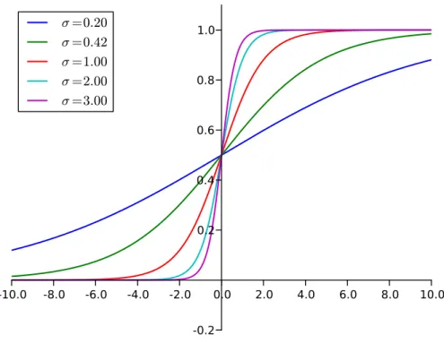
3.2 The generalized logistic function. . . 25

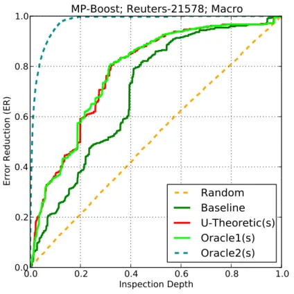
3.3 Error reduction, measured asERM

ρ , as a function of validation depth.

The dataset is _{Reuters-21578}, the learner is_MP-Boost. The

Randomcurve indicates the results of our estimation of the expected

ERof the random ranker via a Monte Carlo method with 100 random

trials. Higher curves are better. . . 32

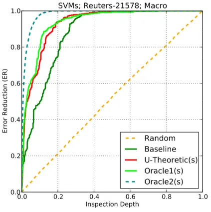
3.4 Same as Figure 3.3, but with the SVM learner in place of_MP-Boost. 40

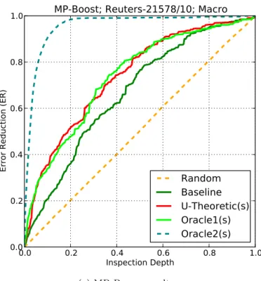
3.5 Results obtained by (i) splitting the_{Reuters-21578}test set into 10

random, equally-sized parts, (ii) running the analogous experiments of Figure 3.3 independently on each part, and (iii) averaging the results across the 10 parts. . . 43

3.6 Same as Figure 3.5 but with _{Reuters-21578/100} in place of

(14)

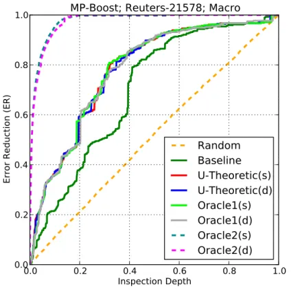
4.1 Error reduction, measured asERρM, as a function of validation depth.

The dataset is Reuters-21578, the learner isMP-Boost. The

Randomcurve indicates the results of our estimation of the expected

ERof the random ranker via a Monte Carlo method with 100 random

trials. Higher curves are better. . . 57

4.2 Same as Figure 4.1, but with the SVM learner in place of_MP-Boost. 58

4.3 Results obtained by (i) splitting theReuters-21578test set into 10

random, equally-sized parts, (ii) running the analogous experiments of Figure 4.1 independently on each part, and (iii) averaging the results across the 10 parts. . . 59

4.4 Same as Figure 4.3 but with _{Reuters-21578/100} in place of

Reuters-21578/10. . . 59 4.5 Error reduction, measured asERµ_ρ, as a function of validation depth.

The dataset is_{Reuters-21578}, the learner is_MP-Boost. . . 68

5.1 Results for macro-averagedF1 of active learning runs, the evaluation

is made onT e, learners are_MP-Boost(5.1a and 5.1c) and SVMs

(5.1b and 5.1d), datasets are_{Reuters-21578} (5.1a and 5.1b) and

OHSUMED-S(5.1c and 5.1d). . . 81

5.2 Results for micro-averaged F1 of active learning runs, the evaluation

is made onT e, learners are_MP-Boost(5.2a and 5.2c) and SVMs

(5.2b and 5.2d), datasets are_{Reuters-21578} (5.2a and 5.2b) and

5.3 Results for macro-averaged error reduction of active learning methods

applied on SATC, for learnersMP-Boost(5.3a and 5.3c) and SVMs

(5.3b and 5.3d), on datasetsReuters-21578 (5.3a and 5.3b) and

5.4 Results for micro-averaged error reduction of active learning methods

applied on SATC, for learners_MP-Boost(5.4a and 5.4c) and SVMs

(5.4b and 5.4d), on datasets_{Reuters-21578} (5.4a and 5.4b) and

OHSUMED-S(5.4c and 5.4d). . . 85 6.1 Comparison of the actual and estimatedF₁M andF₁µ on the test sets.

The curves describe the increment inF1 during manual validation of

the test sets. . . 93

6.2 Results obtained on _{Reuters-21578} with _MP-Boost for the

measuresERM

(15)

List of Tables

2.1 Characteristics of the test collections used. From left to right we report the number of training documents (2), the number of test documents (3), the number of classes (4), and the average number of classes per test document (5). Columns 6-9 report the initial accuracy (bothF1M andF

µ

1) generated by theMP-Boostand SVMs classifiers. 18

3.1 Results of various ranking methods, applied toMP-Boostand several

test collections, in terms ofEN ERM

ρ (ξ), for ξ∈ {0.05,0.10,0.20}. Improvements listed for the various methods are relative to the

baseline. _{Reuters-21578/10} and _{Reuters-21578/100} are

respectively named as_R-21578/10and _R-21578/100. . . 38

3.2 Results of various ranking methods, applied to SVMs and several

test collections, in terms ofEN ERM_ρ (ξ), for ξ∈ {0.05,0.10,0.20}. Improvements listed for the various methods are relative to the

baseline. _{Reuters-21578/10} and _{Reuters-21578/100} are

respectively named as_R-21578/10and _R-21578/100. . . 39 3.3 Characteristics of the test collections used. From left to right we

report the number of test sets (Column 2) and, for each test set, the number of training documents (3), the number of test documents (4), the number of classes (5), and the average number of classes per test

document (6). Columns 7-10 report the initial error (both EM

1 and

E₁µ) generated by the_MP-Boostand SVMs classifiers. . . 41

4.1 Results of various ranking methods, applied to_MP-Boostand several

test collections, in terms ofEN ERMρ (ξ), forξ∈ {0.05,0.10,0.20}. . . . 60

4.2 Results of various ranking methods, applied to SVMs and several test

collections, in terms ofEN ERM

ρ (ξ), forξ∈ {0.05,0.10,0.20}. . . 61

4.3 Comparison between the actual computation times (in seconds) of the

U-Theoretic(s)andU-Theoretic(d)methods on our five datasets. . . 62

4.4 As Table 4.1, but withEN ERµ

(16)

4.5 As Table 4.2, but withEN ERρµ(ξ) in place ofEN ERMρ (ξ). . . 67

5.1 Results of ranking methods based on active learning strategies, applied

to_MP-Boostand SVMs, on_{Reuters-21578} and_OHSUMED-S,

in terms ofEN ERM

ρ (ξ), for ξ ∈ {0.05,0.10,0.20}. Improvements

listed for the various methods are relative to the baseline. . . 86

5.2 Results of ranking methods based on active learning strategies, applied

toMP-Boostand SVMs, onReuters-21578 andOHSUMED-S, in terms ofEN ERµ_ρ(ξ), forξ∈ {0.05,0.10,0.20}. Improvements listed for the various methods are relative to the baseline. . . 87

6.1 Comparison of learners effectiveness and estimated FM

1 and F

µ

1.

Datasets are indicated as_Rfor_{Reuters-21578},_Ofor_OHSUMED

and _O-S for _OHSUMED-S. In the first column we indicate the evaluation of the classifiers onT e, in the second column we indicate the evaluations estimated onT rvia 10-fold cross-validation, and in the third column we indicate the estimated evaluation after the total manual validation ofT e. . . 94

6.2 Errors generated by the_MP-Boostand SVMs classifiers, evaluating

the classification accuracy withF0.5 andF2. . . 96

6.3 Results of ranking methods applied to MP-Boostand SVMs, on

Reuters-21578, OHSUMED and OHSUMED-S, in terms of

EN ERµ₀_.₅(ξ), for ξ∈ {0.05,0.10,0.20}. Improvements listed for the

various methods are relative to the baseline. . . 98

6.4 Results of ranking methods applied to _MP-Boostand SVMs, on

Reuters-21578, OHSUMED and OHSUMED-S, in terms of

EN ERµ₂(ξ), for ξ∈ {0.05,0.10,0.20}. Improvements listed for the

6.5 Results of ranking methods applied to _MP-Boostand SVMs, on

Reuters-21578, Reuters-21578/10andReuters-21578/100, in

terms ofEDN ERM

ρ (ξ), forξ∈ {0.05,0.10,0.20}. Improvements listed for the various methods are relative to the baseline. . . 103

6.6 Results of ranking methods applied to SVMs, on Reuters-21578,

Reuters-21578/10 and Reuters-21578/100, in terms of

EDN ERµ

ρ(ξ), forξ∈ {0.05,0.10,0.20}. Improvements listed for the various methods are relative to the baseline. . . 104

(17)

6.7 Characteristics of the ten market research datasets (LL-A to LL-L), four customer satisfaction datasets (Egg-A1 to Egg-B2), and one social science dataset (ANES L/D), that we have used here for experimentation. The columns represent the name of the dataset, the number of training verbatims (|T r|) and the number of test verbatims (|T e|), the number of codes in the codeframe (|C|), the average

number of positive training verbatims per code (AV C), the average

training verbatim length (AV L), and the initial error (bothEM

1 and

E₁µ) generated by the_MP-Boostand SVMs classifiers. . . 105

6.8 Results of SATC ranking methods on survey datasets, in terms of

EN ERM

ρ (ξ), for ξ∈ {0.05,0.10,0.20}. Improvements listed for the

6.9 Results of SATC ranking methods on survey datasets, in terms of

EN ERµ

ρ(ξ), for ξ∈ {0.05,0.10,0.20}. Improvements listed for the

(18)

(19)

1 Introduction

Textual data is present in our everyday activities, e.g., when we read the news on the Web, when we fill out paperwork, etc. Analyzing textual data is an important activity in many scenarios of our society, but it sometimes involves difficult challenges that we can barely manage with human effort only. One of the main problems in text analysis is that texts are now generated at high rates, thus it is often the case that the size of the data forces us to entrust this analysis to computing systems.

There is a high demand of automatic systems for extracting information and un-derstanding the content of textual data. The need of structuring knowledge from texts can be tackled computationally, so in the last years many research studies in informa-tion technology have pushed forward the state of the art oftext mining technologies. Several tasks make up the text mining field, and for each task different approaches have been proposed to solve them. Applications of text mining usually have to follow specific requirements, which are imposed by the need of extracting or accessing partic-ular types of information. The challenge for a researcher is to find and apply the right methods, in order to optimize the effectiveness and the efficiency of the applications. Modern search engines are a popular application for automatic access to textual data. Search engines are a solution to the activity ofinformation retrieval(IR) [54, 78]. A retrieval application has to answer the information need of a user, by exploring and identifying the relevant data. Information retrieval embraces a wide area of the text mining research and the impact of IR research is huge in our society. Sometimes a text mining application has to meet more specific requirements, which do not respond to a generic need as in the case of search engines. Some applications answer the demand of a single customer, or they are applied on particular textual data, publicly accessible or private. This scenario is more common for today’s large organizations and industries, which are faced with the need of processing large amounts of textual data in order to understand the satisfaction of their clients or to manage their own knowledge bases.

(20)

CHAPTER 1. INTRODUCTION

1.1 Text classification

Suppose an organization needs to classify a setDof textual documents under a classi-fication schemeC, that consists of a set of labelscj∈ C, each of which can be assigned or not to any of the documents di ∈ D. Suppose that Dis too large to be classified manually, so that resorting to some form of automatedtext classification (TC) [2, 73] is the only viable option. TC is the activity of automatically labelling natural lan-guage texts with thematic classes (or categories or labels) from this predefined set

C.

In this task the knowledge we can access is in the form of textual documents, and no other information is available. The categories are just symbolic labels, and they identify a set of documents according to some predefined criteria. One could group documents by topic, by opinion, or according to other aspects, depending of the TC application; some examples of applications are:

• the categorization of news articles, where documents are classified according to

the topic they deal with (e.g., politics, sport, etc.), or are filtered according to the profile of the user [42];

• spam filtering [15], in which the TC application is integrated in the e-mail client,

so that the e-mails automatically labelled as spam are filtered out by the client;

• sentiment classification [52], in which TC is used together withcomputational

lin-guistic technologies, in order to label documents (e.g., product reviews or political

debates) according to the opinions they contain.

Typical applications of TC are in scenarios where a large quantity of documents has to be analyzed, and the human cost needed to manually perform the annotation is, most of the times, prohibitive. TC applications may be not as accurate as human labellers, but they are cheaper and surely more efficient.

The TC task can be further characterized depending on the desired application. For example, one might accept that any number of categories can be assigned to a document; this is the multi-label case of TC. Alternatively, or one could restrict this number to one, so that exactly one category from the set must be assigned to a doc-ument (thesingle-label case). In general these characteristics are parameters of a TC

framework. The modern and effective approach to TC is throughsupervised learning.

A TC framework built on supervised learning algorithms works in two phases: (i) it receives in input the setC and a set of documents, labelled with the categories inC (the so-calledtraining data); it learns from the data, understanding the characteristics which link the documents to the categories, and it models the learned information into

a classifier; (ii) the classifier performs the automatic classification of the documents

inD, according to the categories inC.

The effectiveness of a classifier is dependent of the information on which it is built. The quality of the training data, that is usually generated manually, and the choice of the algorithm and its parameters determine the accuracy of the classifier.

(21)

1.2. SEMI-AUTOMATED TEXT CLASSIFICATION But what if, as a consequence, the customer is not satisfied by the accuracy of the automatic classification? What if the customer is willing to do, or pay for, a part of the classification manually? We answer these questions by introducing a novel scenario for text classification.

1.2 Semi-automated text classification

Suppose that an organization which needs to classify documents has strict accuracy standards, so that the level of effectiveness obtainable via state-of-the-art TC tech-nology is not sufficient. In this case, the most plausible strategy to follow is to classify

the setDof documents by means of an automatic classifier (which we assume here to

be generated by a supervised learning algorithm), and then to have a human editor validate (i.e., inspect and correct where appropriate) the results of the automatic

clas-sification. The human annotator will obviously validate only a subsetD0 _{⊂ D}_(since

it would not otherwise make sense to have an initial automated classification phase), e.g., until she is confident that the overall level of accuracy ofDis sufficient, or until she has time. We call this scenariosemi-automated text classification (SATC).

An automatic TC system may support this task by ranking, after the classification phase has ended and before the validation begins, the classified documents in such a way that, if the human annotator validates the documents starting from the top of the ranking, the expected increase in classification effectiveness that derives from this validation is maximized.

In this dissertation we will devise effective ranking strategies for this task, and we will explore the feasibility of SATC applications and their integration into TC systems.

Anyone already familiar with TC technologies might ask: why not just useactive

learning? In active learning (AL) [74] the human effort is spent for annotating new

documents (typically from the set of automatically labelled documents), which are added to the training data in order to learn from a richer set of documents. The goal of SATC is not improving classifier quality, but directly improving the accuracy of the set of automatically classified documents. The human validation typical of

SATC comes after the automatic classification phase, guarantees a positive gain in

effectiveness, which is a strict requirement.In this dissertation we will investigate the relationship between SATC and AL.

Another question can come to mind: is there a real need for SATC applications? The answer is yes, there are multiple scenarios in which automatic classification and human intervention both play a role, and we will discuss them in this dissertation. An example task in which human validation is a critical phase ise-discovery [29, 63]. E-discovery is a process, in a legal case, where one party has to make available to the other the digital material in its possession that is pertinent with the case. This material is often in the form of textual data, and the size of these data makes this task difficult to process by means of manual work only. The process of reviewing

(22)

the documents is oftentechnology-assisted, and split in several steps: in a first phase a subset of documents is retrieved and annotated according to its relevance to the case, then a classifier is built so as to find the maximum possible number of relevant documents. The final goal is to produce an accurate classification of relevant and non-relevant documents, with a continuous interaction of human reviewers throughout the process. Documents are usually ranked, for presentation to the reviewers, by means of their relevance (computed from the classification output scores), so as to optimize the reviewers’ work. In this scenario SATC seems to be the right solution for optimizing the manual, expensive work of human labelling. In fact, ranking documents by relevance is suboptimal (as we will show in this dissertation), if the objective is validating the classification process. We can thus realize that SATC is applicable in any process that involves the automatic analysis of data with the support of human validators.

1.3 Our contribution

An obvious strategy for a SATC method is to rank the documents in ascending order of the confidence scores returned by the classifier. In fact, classifiers based on supervised learning algorithms usually output a real value along with the classification decision, which is proportional to their confidence in the decision. By employing this strategy, the top-ranked documents are the ones that the classifier has labelled with the lowest confidence. We call this strategy “obvious” because of the evident similarities between SATC and active learning, where this strategy is an often used baseline. However, to the best of our knowledge, the application of this ranking method (or of any other ranking method, for that matter) to SATC has never actually been discussed in the literature. The rationale for this method is that an increase in effectiveness can derive

only by validatingmisclassifieddocuments, and that a good ranking method is simply

the one that top-ranks the documents with the highest probability of misclassification, which (in the absence of other information) we may take to be the documents which the classifier has categorized with the lowest confidence.

In this work we show that this strategy is, in general, suboptimal. Simply stated, the reason is that the improvements in effectiveness that derive from correcting a false positive (an erroneous assignment of a class) or a false negative (an erroneous non-assignment of a class) may not be the same, depending on which evaluation function we take to represent our notion of “effectiveness”. Additionally, the ratio between these improvements may vary during the validation process. In other words, an optimal ranking strategy must take into account the above improvements and how these impact on the evaluation function; we will thus look at ranking methods based

on explicit loss minimization, i.e., optimized for the specific effectiveness measures

used.

(23)

1.4. STRUCTURE OF THE THESIS

• we develop new utility-theoretic ranking methods for SATC based on the notion

of validation gain, i.e., the improvement in effectiveness that would derive by

correcting a given type of mistake (i.e., false positive or false negative);

• we introduce a further ranking method, which is based on the notion of “dynamic”

adjustment of validation gains;

• we formulate the above ranking methods for two different methods of averaging

classification accuracy across different classes;

• we propose a new evaluation measure for SATC, and use it to evaluate our

exper-iments on standard datasets;

• we perform a number of analyses and extensions of the methods above and the

evaluation measures above, and we apply our SATC methods in different applica-tion contexts.

The results of all the experiments in this dissertation show that, with respect to the confidence-based baseline method above, our ranking methods are substantially more effective.

This dissertation presents, to the best of our knowledge, the first systematic work on the task of semi-automated text classification. This work has resulted in the fol-lowing scientific publications:

I) A utility-theoretic ranking method for semi-automated text classification. Gia-como Berardi, Andrea Esuli, and Fabrizio Sebastiani. InProceedings of the 35th International ACM SIGIR Conference on Research and Development in

Infor-mation Retrieval (SIGIR 2012), Portland, US. This is The first technical paper

we have published on the topic.

II) Optimising Human Inspection Work in Automated Verbatim Coding. Giacomo

Berardi, Andrea Esuli, and Fabrizio Sebastiani. International Journal of

Mar-ket Research. To appear. This is a paper which introduces SATC in

easy-to-understand terms to a non-specialized audience (market researchers) of potential users of this technology.

III) Utility-Theoretic Ranking for Semi-Automated Text Classification. Giacomo Be-rardi, Andrea Esuli, and Fabrizio Sebastiani.ERCIM News, 2013(92). This is an extended abstract of I), published in an international computer science bulletin. IV) Utility-Theoretic Ranking for Semi-Automated Text Classification. Giacomo

Be-rardi, Andrea Esuli, and Fabrizio Sebastiani. Submitted to ACM Transactions

on Information Systems. This is a substantially revised and extended version of

I), submitted to the top information retrieval journal.

1.4 Structure of the thesis

The dissertation is organized as follows.

In Chapter 2 we describe how automated text classification is actually achieved. We introduce preliminary definitions, notations, and the approach to TC by means

(24)

of supervised learning. We thus describe algorithms, evaluation measures, and data collections that we use as the core in the development of SATC methods.

In Chapter 3 we introduce our approach to SATC. We describe our basic utility-theoretic strategy for ranking the automatically labelled documents. Furthermore, we propose a novel effectiveness measure for this task based on a probabilistic user model. We report the results of our experiments in which we test the effectiveness of ranking strategies by simulating the work of a human annotator who validates variable-sized portions of the labelled test set. Finally, we propose some further readings about the discussed subjects.

In Chapter 4 we address a potential problem deriving from the “static” nature of our strategy, by describing a “dynamic” (albeit computationally more expensive) version of the same strategy, and draw an experimental comparison between the two. Then we acknowledge the existence of two different ways (“micro” and “macro”) of averaging effectiveness results across classes, and show that the methods we have developed so far are optimized for macro-averaging; we thus develop and test methods optimized for micro-averaged effectiveness.

In Chapter 5 we investigate the task of active learning and its relationships with SATC. We look at the common aspects and the differences of the two tasks. We compare methods specific to AL or SATC in two steps: first we test our SATC ranking methods in an AL scenario, then we apply AL methods to a SATC setting.

In Chapter 6 we further explore the potential of our SATC methods, facing a number of subtasks: first we try to determine if we can dynamically estimate the achieved level of accuracy of the classification, which is a central aspect of a SATC application. We then study other classification accuracy measures, and a new variant of our evaluation function for SATC. We finally we apply SATC ranking methods in the context of automatic classification of market research surveys.

(25)

2 Text Classification

In this chapter we describe the basic notions and the methods for performing auto-matic text classification [2, 73]. Along the chapter we introduce the notation used in this dissertation.

Given a set of textual documents Dand a predefined set of classes (or categories) C={c1, . . . , cm},multi-class multi-label TC is usually defined as the task of estimat-ing an unknowntarget function Φ:D × C → {−1,+1}, that describes how documents ought to be classified, by means of a function ˆΦ:D × C → {−1,+1} called the

clas-sifier1_{; +1 and} ₋_{1 represent membership and non-membership of the document in}

the class. Here, “multi-class” means that there arem≥2 classes, while “multi-label” refers to the fact that each document may belong to zero, one, or several classes at

the same time. Multi-class multi-label TC is usually accomplished by generating m

independent binary classifiers ˆΦj, one for eachcj ∈ C, each entrusted with deciding whether a document belongs or not to a classcj.

In this dissertation we will actually restrict our attention to classifiers ˆΦj that, aside from taking a binary decision Dij ∈ {−1,+1} on a given document di, also return a confidence estimate Cij, i.e., a numerical value representing the strength of their belief in the fact that Dij is correct (the higher the value, the higher the confidence). We formalize this by taking a binary classifier to be a function ˆΦj :D →R

in which the sign of the returned valueDij ≡sgn( ˆΦj(di))∈ {−1,+1} indicates the binary decision of the classifier, and the absolute valueCij ≡ |Φˆj(di)| represents its confidence in the decision.

2.1 Supervised learning

In order to obtain the classifier ˆΦwe use a Machine Learning (ML) approach to TC.

In ML a classifier is estimated through an automatic process of learning. The learner builds a classifier by observing the documents that a human annotator, who is an

1

Consistently with most mathematical literature we use the caret symbol (ˆ) to indicate estimation.

(26)

CHAPTER 2. TEXT CLASSIFICATION

expert in the domain of the considered textual data, has classified. For a categorycj

the learner analyzes the characteristics of the documents labelled with both cj and

¯

cj. This inductive process models the characteristics that a new, unseen, document

should have in order to be classified under cj. This solution to classification is also known as supervised learning, that is the activity of learning under the supervision of the knowledge extracted from the set of training documents. The key aspect for building an effective classifier is in the available resources, these are the documents in

Dand the categories inC, which are assigned to the documents. The data resources

are usually provided by the customer of the classification service, an organization or a company, that owns a knowledge base and wants to automate the activity of extending this knowledge.

In supervised learning we need an initial, classified, set of documents D =

{d1, . . . , d|D|} ⊂ D. Documents in D are classified under C, so the values of Φ are

known for each pair hdi, cji ∈ D × C. This set is used for two fundamental goals: (i) building the classifier, that is eventually used on new documents; (ii) tuning and evaluating the classification model.

In a common experimental setting, D is divided in two subsets:

• The training set T r ={d1, . . . , d|T r|} ⊂D, that is used in thelearning process,

namely the construction of the classification model;

• The test setT e={d|T r|+1, . . . , d|D|} ⊂D, that is used for evaluating the classifier

ˆ

Φ built on T r. The evaluation of the effectiveness of the classifier is performed comparing the values of sgn( ˆΦ(di)) against the values of sgn(Φ(di)), for each

di∈T e.

The key aspect of this experimental setting is that the classification model is built working exclusively onT r. The purpose is to simulate a real scenario in which we do not know anything about the documents to be classified, as those belonging toT e.

The effectiveness of a classifier can be estimated on T r through a k-fold cross-validation. In this approachT r is divided ink partitions, sok experiments are

con-ducted using the training/test approach. The validation is composed ofk

learning/-classification stages, i.e.kclassifiers are built and evaluated on the training and test set pairs hT ri =D−T ei, T eii,∀i ∈ [1, k]. The final evaluation is computed as the average of thekevaluations performed on every T ei. In some learning algorithms it is possible to set parameters in order to adjust the specific behaviors of the learners. The k-fold cross-validation is a solid tool for exploring and selecting the parameter values: a validation is performed for each value, the best parameter values are the ones for which thekclassifiers have the best average effectiveness.

In the next sections we introduce in detail the techniques for analyzing and repre-senting textual data; two ML algorithms are discussed: SVMs and Boosting. Finally the reference evaluation measures are presented. All these elements, with the ex-perimental methodology discussed above, are the basis of SATC methods and their evaluation.

(27)

2.1. SUPERVISED LEARNING 2.1.1 Text representation

Text semantics have to be represented in a form that can be interpreted by the ML

algorithms. Documents are passed under a process of indexing, that is performed

uniformly for all the documents in D. In this process the meaningful units of the

texts are identified and each document is converted to a numerical representation. In TC each sample of the data is a document, and it is represented by a vector; each component of a document vector is a feature, and its value defines the feature weight; features are units, characteristics, which describe a document. The most common features for texts are the terms of the documents; a term can be identified as a word, so a term weight can be defined as the importance of the word for a document.

In the learning phase we identify the features from the available data, represented by the training set. In the vector space of documents each dimension is a term of the dictionary drawn fromT r, so the representation ofdi is di =hw1i, . . . , w|T |ii where T is the dictionary, namely the set of terms that occur at least once in at least one

document of T r. If the dictionary is made of words, we call this approach Bag of

Words (BOW). Word weights can be binary (i.e. 0 or 1 is the word is respectively present or not in the document) or real values:wki ∈ [0,1]. The higher the weight, the greater is its contribution to the semantics of a document. With this approach words are taken as independent units, discarding the semantic dependencies of the language, which are not employed by the learners.

In order to obtain document vectors, a function for computing weights is necessary.

In the case of binary weights we simply set wki to 1 if the term tk occurs in the

document di. A richer semantic could be the number of occurrences of the term,

this measure is usually calledterm frequency, defined by the function tf(tk, di). The intuition behind the term frequency is that the representativeness of a term for a document is directly proportional with its frequency in that document. The problem with term frequency is that the most common terms of a language, like prepositions,

conjunctions, etc., have high tf in every document. The same is true for the most

common terms of a specific domain, e.g. the word “game” is very frequent in a training set about the subject “sport”. In order to mitigate this problem, we can weight the term frequency by the inverse of the document frequency. The importance of a term is then a combination of its occurrences in the documents and its occurrences in the whole training set. The functiontf idf [70] is defined as

tf idf(tk, di) =tf(tk, di)·log

|T r|

df(tk)

where df(tk) is the number of documents in T r in which tk occurs. An alternative weighting function is the normalized tf idf, which returns values that fall in [0,1] interval. We can normalize the document vectors through the cosine normalization:

wki=

tf idf(tk, di) q

P|T |

(28)

In the BOW approach some preprocessing steps are usually performed before the vectorization of documents. Textual data is cleaned in order to keep only the useful semantics and discards useless units of text, the standard process consists in filtering

out punctuation and stop words. Stop words are the elements of a language that

are used for the construction of the syntax, which do not carry useful semantics: articles, prepositions, conjunctions, “to be”, “to have”, etc. A successive common preprocessing step isstemming, in which words are reduced to their stem, base or root form. Multiple words can be related to the same stem (e.g. “logically” and “logics” are related to “logic”), by using stems we obtain a more compact and meaningful representation of the document semantics.

2.1.2 Support vector machines

Support vector machines (SVMs) [16] are supervised learning algorithms that learn from the training data by separating the space of the samples according to their classes. A SVMs learner builds ahyperplanein the multi-dimensional space of features, which better separates the samples that belong to a class from the others (binary classification case). The optimal separation is the one that brings about the largest margin between the hyperplane and the samples of both sides. The closest samples

to the hyperplane are called the support vectors, as they alone define the decision

boundary between the two sides.

One big advantage of SVMs is their modularity, that allows to train the model on samples that are not linearly separable. In TC it is common to explore only linear solutions (linear SVMs), as they have proven to be effective [17]. SVMs have been adopted in TC [36, 37] for their favorable characteristics: they behave efficiently for high dimension space inputs; they can handle irrelevant features and very sparse vectors, two aspects that are very common in textual data; it is possible to easily

tune a SVM learner in order to overcome the problem ofoverfitting. However, SVMs

are generally effective in TC with the standard setting of their parameters.

Multi-class multi-label TC with SVMs can be achieved employing the binary clas-sification approach, so we build an independent classifier for each class cj. In the

vector space of documents we can define any hyperplanehas

w·d−b= 0

For each categorycj, and any documentdi inD, we want to find a hyperplane such as

wj·di−bj ≥+1 if Dij = +1 wj·di−bj ≤ −1 if Dij =−1 This can be rewritten as:

Dij(wj·di−bj)−1≥0

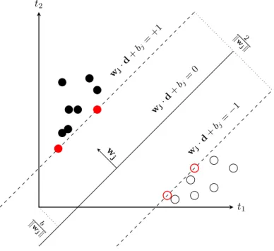
The points that intersect the planesh+1:wj·di−bj = +1 andh−1:wj·di−bj = +1 are the support vectors, they are marked in red in Figure 2.1.

(29)

2.1. SUPERVISED LEARNING t2 t1 wj ·d +b j= 0 wj ·d+ bj= +1 wj ·d +b j= −1 2 k_w jk b k_w j_k w j

Figure 2.1: An example of a hyperplane which brings the largest separation margin of documents for classcj. The vector space has two dimensions for termst1andt2.

In order to find the best hyperplane, i.e. the one for which the distance between it and the support vectors is maximum, we solve an optimization problem. We search for the vectorwj that maximizes the distance fromh+1 to the hyperplaneh, that is equivalent to the distance betweenh−1 andh:

wj·di−bj

kwjk

= 1

kwjk

The problem to be solved is a minimization problem, with the constraints defined by the samples of the training set:

min (wj,bj)

kwjk s.t.:

Dij(wj·di−bj)−1≥0 ∀di∈T r We can alter the initial function min

(wj,bj)

kwjkinto min

(wj,bj)

1 2kwjk

2_{, thus the optimization} problem is transformed in a quadratic programming problem, which can be solved with the method of Lagrange multipliers [16].

After the optimal separation is found, we can classify new documents according to their relative position to the hyperplane. In the learning phase we obtain the param-eters of the function ˆΦj(di) =wjbest·di−bbestj , that returns strictly positive values if the documentdiis classified with the classcj, strictly negative values otherwise. The

(30)

function returns 0 if the document lies on the hyperplane. The confidence of classifi-cation is then proportional to the distance of the document point from the decision boundary defined by the optimal hyperplane.

In [16] the authors introduce a further parameter into the learning algorithm, in order to manage noisy points - outliers that can negatively affect the decision bound-ary. TheCparameter plays a role of regularization of the function to be minimized; it controls the relative importance of minimizingkwjk, that is equivalent to controlling

the size of the margin. When we assign toCvalues close to 0, we allow samples near

the decision boundary to violate the constraints of the minimization problem, so the learner excludes points that can easily overfit the model on the training data. The

opposite happens when we setCto values close to∞, the constraints imposed on the

training samples are strictly followed in the solution of the optimization problem.

2.1.3 Boosted decision trees

The family of ML algorithms called boosting algorithms is based on the principle of

combining several learners, in order to produce one effective classifier. The typical boosting method starts by creating weak classifiers, models whose classification effec-tiveness is low. Weak classifiers are usually built learning only a few (limited) aspects of the training data, consequently their classification accuracy is limited. In boosting several weak classifiers are built with the final goal of combining them in a global strong classifier, that is able to deal with all the characteristics of the data.

One popular variant of boosting is AdaBoost, its name stands for Adaptive Boost-ing. In AdaBoost weak classifiers are built iteratively, each one is tuned in order to perform better on the data that the previous weak classifier has misclassified, the algorithm adapts itself to the training data.

A variant of AdaBoost is _MP-Boost [19], that is an improved version of

Ad-aBoost.MH[72]. These two variants are optimized for multi-label classification, the

weak classifiers they create are decision trees, trained on specific terms. Each weak classifier is built around a pivot term and sets up its classification on the presence or the absence of the term in the document (binary feature weights). The improvement of MP-Boost, compared toAdaBoost.MH, is in how pivot terms are chosen. At each iteration, more pivot terms are selected, one for each class. The algorithm then constructs a set of weak classifiers at each iteration, each of them is optimized for a specific class.

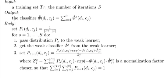
MP-Boost algorithm

In MP-Boost weak classifiers are generated iteratively, so if S is the number of iterations, we have ˆΦ1_{. . .}_ΦˆS _{weak classifiers. At the end of each iteration the final} classifier is obtained summing up the weak classifiers ˆΦ = PS_s₌₁Φˆs_{, so both the}

(31)

2.1. SUPERVISED LEARNING

Input:

a training set T r, the number of iterationsS

Output: the classifier ˆΦ(di, cj) = PS s=1Φˆ s₍_d i, cj) Body: set P1(di, cj) = _|_{T r}1_|·|C| fors= 1, . . . , S do:

1. pass distributionPsto the weak learner;

2. get the weak classifier ˆΦs_{from the weak learner;} 3. setPs+1(di, cj) = Ps(di,cj)·exp(−Φ(di,cj)·Φˆsj) Zs j whereZs j = P|T r|

i=1 Ps(di, cj)·exp(−Φ(di, cj)·Φˆsj) is a normalization factor chosen so thatP|T r|

i=1

P|C|

j=1Ps+1(di, cj) = 1

Figure 2.2: The _MP-Boostalgorithm

confidence estimates and the classification decisions of ˆΦare obtained from the sum of the values of the single weak classifiers.

The algorithm (Figure 2.2) creates a weak classifier for each class at each iteration, then we have |C| weak classifiers at each iteration. For class cj, at iteration s, the classifier ˆΦs

j is built.MP-Boostupdates a distribution of weights on the training set

pairshdi, cjiat each iterations. We definePs+1as the distribution that is used by the algorithm at iterations+ 1. The value ofPs+1(di, cj) is updated in order to capture the effectiveness of the classifiers ˆΦ1_j. . .Φˆs_j in assigning classcj to the document di. The weights are proportional to the ability of the classifiers of correctly assigning the class, the higher the weight, the more difficult the assignment. The weak classifier

ˆ

Φs_j+1, in order to better classify documents with higher weights, concentrates on those features that allows to better discriminate the classcj. Every weak learner at iteration

s+ 1 takes in input the training set and the distributionPs+1.

The initial distributionP1is uniform; at iterationsweights are updated according to: Ps+1(di, cj) = Ps(di, cj)·exp(−Φ(di, cj)·Φˆsj) Zs j where Z_js= |T r| X i=1 Ps(di, cj)·exp(−Φ(di, cj)·Φˆsj)

is a normalization factor, so Ps+1(di, cj) is a distribution, the sum of all the weight values is 1.

A weight is updated proportionally to its previous value, it is increased if the

(32)

−Φ(di, cj)·Φˆsj is positive if the target function and the weak classifier have differ-ent sign, in this case the expondiffer-ential functionexpis≥1.

MP-Boost weak classifiers

Text is represented with binary feature weights. The weightwkiof a document vector

di is equal to 1 if the term tk is contained in the document, 0 otherwise. A weak

classifier ˆΦs

j is a decision tree, with only one root and two leaves. It returns a specific real value if a term is present in the document and a different value if it is not. The term is calledpivot term, thus we have|C|pivot terms at each iteration s. The weak classifier is defined as ˆ Φs_j(di) = aj₀ifwj_ki= 0 aj₁ifwj_ki= 1

Creating a weak classifier means choosing a termtj_k and the valuesaj₀ andaj₁. These three parameters are obtained during the learning phase, that consists in minimizing the error of the weak classifier. This error can be measured by the normalization factorZs

j.

In order to obtain ˆΦs_j these two steps are executed (at iterations): 1. Select among all ˆΦs

j that have a specific term as pivot term, the one which mini-mizesZs

j. In this step we create |T |weak classifiers, and for each one we choose the values aj₀andaj₁.

2. Select among all the best weak classifiers previously created, the one which mini-mizeZ_js. In this step we choose the unique pivot termtj_kfor the current iteration. The first step is critical, since we can not enumerate all the possible values ofaj₀ and

aj₁._MP-Boostdeals with this step using the same approach of_AdaBoost.MH; this approach is argued in [71], where the authors have proven that:

ˆ Φbest_j (k)(di) =      1 2log W₊₁0jk W₋0jk₁ ifw j ki= 0 1 2log W₊₁1jk W₋1jk₁ ifw j ki= 1

where best(k) denotes the best weak classifier for termtj_k, selected at the first step, and where W_bxjk= |tr| X i=1 Ps(di, cj)·Jw j ki=xK·JΦ(di, cj) =bK

forb∈ {−1,+1},x∈ {0,1}, and where_Jπ_Kis the characteristic function of predicate

π, so ifπis true the function returns 1, 0 otherwise. The valuesW_bxjk are equivalent to the weight, with respect to the distributionPs, of the documents that contain (or does not contain) the termtj_k, which are classified (or are not) withcj.

Reminding that ˆΦs(di, cj)≡Φˆsj(di), the final classifier is ˆΦ(di, cj) = PS

s=1Φˆ

s₍_d i, cj),

where S is the number of iterations (the only free parameter of MP-Boost

algo-rithm). The classification values are thus a combination of the valuesaj₀andaj₁of the pivot terms of each iteration.

(33)

2.2. EVALUATING TEXT CLASSIFICATION

2.2 Evaluating text classification

Several measures exist for evaluating the accuracy of text classifiers. It is possible to estimate the accuracy of a classifier during the learning phase, performing a validation step (e.g. k-fold cross-validation). While these operations are performed on T r, the

final evaluation is executed on T e. We use T e in order to simulate a “production”

phase, in which the classifier is applied on new, unseen and unlabelled documents. The evaluation scores we obtain onT eare used for comparing the classifier effectiveness. We implicitly refer to the evaluation onT ehereafter.

In a classification task, for each assignment of a class to a document, we can define four possible events, according to the true label of the document. We can obtain a true positive, a true negative, a false positive or a false negative. The terms “positive” and “negative” refer to the predicted assignment made by the classifier, while “true” and “false” refer to the correctness of the prediction with respect to the real assignment of the document. We useT P(ij) to indicate that ˆΦj(di) is a true positive, and useF P(ij) (false positive),F N(ij) (false negative), andT N(ij) (true negative) with analogous meanings; e.g. ifT N(ij) is true, then the classifier has correctly not assigned the class

cj to the documentdi.

With T Pj,F Pj, F Nj, and T Nj we indicate the numbers of true positives, false positives, false negatives and true negatives in the test set T e for category cj. The

four values can be formulated in a contingency table as in Figure 2.3, each value is

represented in acontingency cell.

predicted

Y N

true Y T P = 4 F P = 3

N F N= 4 T N= 9

Figure 2.3: An example of a contingency table of a single-label classification ofT P+

T N+F P+F N = 20 documents.

2.2.1 Evaluation measures

The well known notions ofprecision andrecall in Information Retrieval, can be

de-signed as evaluation measures in TC. The two measure can be formulated on the contingency table: precisionj( ˆΦj(T e)) = T Pj T Pj+F Pj recallj( ˆΦj(T e)) = T Pj T Pj+F Nj

(34)

For a class cj, precisionj is the fraction of correct positive predictions on all the positive predictions, while recallj is the fraction of correct positive predictions on

the number of documents inT ebelonging to cj. The values of both functions range

between 0 (worst) and 1 (best).

Precision and recall can have different priority in the evaluation of a TC system, according to the type of application we evaluate. An example of application that gives precedence to precision is the classification of medical reports, where the category set is made of diagnosable diseases. Assigning the right classes is critical for choosing the right treatment. An example of application that requires high recall is the e-mail spam filter, where e-mails are classified as positive if they are not spam. In this case high recall means low probability that good e-mails are wasted in the spam folder.

A measure that combines precision and recall is the F-measure. The harmonic

mean of precision and recall is defined as theF1 measure:

F1( ˆΦj(T e)) = 2·precisionj·recallj precisionj+recallj = = 2·T Pj 2·T Pj+F Pj+F Nj

F1 is a specific instance of the generic Fβ measure [78]. The parameter β is used to weight the importance of precision over recall, with positive values lower than 1 we put emphasis on precision while with values grater than 1 we put emphasis on recall.

Withβ= 1 we have theF1 defined above.

Fβ( ˆΦj(T e)) = (1 +β2)· precisionj·recallj (β2_·_precision j) +recallj = = (1 +β 2₎_·_{T P} j (1 +β2₎_·_{T P} j+F Pj+ (1 +β2)·F Nj

Note that F1 is undefined when T Pj = F Pj = F Nj = 0; in this case we take

F1( ˆΦj(T e)) = 1, since ˆΦj has correctly classified all documents as negative exam-ples. Note also that in the evaluation based onF1the correct negative classifications are excluded, in fact the function does not embrace the true negative. We will con-centrate on the F1 measure in this dissertation, but it will be successively evident that any kind of measure computed on the contingency table can be used in SATC methods.

We have restricted the discussion of evaluation measures on binary classification. In order to evaluate the effectiveness of multi-class multi-label TC we use two approaches for averaging on the classes:

• macro-averaged F1(notedF1M or macroF1), which is obtained by computing the

class-specificF1 values and averaging them across all thecj∈ C.

F₁M(T e) = P|C|

j=1F1( ˆΦj(T e)) |C|

(35)

2.2. EVALUATING TEXT CLASSIFICATION

• micro-averaged F1 (noted F1µ or microF1), which is obtained by computing the

F1 on a global contingency table, where each contingency cell is the sum of the

respective class-specific contingency cells.

F₁µ(T e) = 2 P|C| j=1T Pj 2P|C| j=1T Pj+ P|C| j=1F Pj+ P|C| j=1F Nj

The two methods of averaging can be applied to any measure, they differ in the im-portance given to the frequency of assigned classes. Macro-averaging weights equally each class; with a macro-averaged measure the evaluation of infrequent classes, which are more likely to produce errors, has the same importance of the evaluation of the most frequent ones. Micro-averaging gives the same importance to each binary clas-sification, so it is independent of the distribution of the classes.

Many evaluation measures exist for classification, in this dissertation we will often use “accuracy of classification” concerning to any measure of effectiveness. We will quantify this definition mostly with theF1measure.

2.2.2 Datasets for text classification benchmarks

Text collections are set of documents and categories made for benchmarking purposes. These collections are publicly available and they come with the true labels assigned to documents, in order to use the entire set of samples for evaluation. They also come with configurations of dataset splitting, in order to define common training and test sets across experiments. TC evaluations are performed choosing datasets together with specific splitting configurations.

Our first dataset is the _{Reuters-21578}[45] corpus. It consists of a set of 12,902 news stories, partitioned (according to the standard “ModApt´e” split we adopt) into a training set of 9603 documents and a test set of 3299 documents. The documents are labelled by 118 categories; the average number of categories per document is 1.08, ranging from a minimum of 0 to a maximum of 16; the number of positive examples per class ranges from a minimum of 1 to a maximum of 3964. In our experiments we restrict our attention to the 115 categories with at least one positive training example. This dataset is publicly available2and it is probably the most widely used benchmark in TC research; this fact allows other researchers to easily replicate the results of our experiments.

Another dataset we use is _OHSUMED [31], a test collection consisting of a set

of 348,566 MEDLINE references spanning the years from 1987 to 1991. Each entry consists of summary information relative to a paper published on one of 270 med-ical journals. The available fields are title, abstract, MeSH indexing terms, author, source, and publication type. Not all the entries contain abstract and MeSH indexing terms. In our experiments we scrupulously follow the experimental setup presented in

2

(36)

[48]. In particular, (i) we use for our experiments only the 233,445 entries with both abstract and MeSH indexing terms; (ii) we use the entries relative to years 1987 to 1990 (183,229 documents) as the training set and those relative to year 1991 (50,216 documents) as the test set; (iii) as the categories on which to perform our experiments

we use themain heading MeSH index terms assigned to the entries. Concerning this

latter point, we restrict our experiments to the 97 MeSH index terms that belong to

the Heart Disease (HD) subtree of the MeSH tree, and that have at least one

pos-itive training example. This is the only point in which we deviate from [48], which experiments only on the 77 most frequent MeSH index terms of the HD subtree.

There are two main reasons why we have chosen exactly these datasets:

1. All of them are publicly available and very widely used in TC research, which allows other researchers to easily replicate the results of our experiments. 2. OHSUMED is one of the largest datasets used to date in TC research, which

lends robustness to our results.

The main characteristics of our datasets are conveniently summarized in Table 2.1. The evaluations on the two collections’ test sets point out the effectiveness of the two

learners. It is clear the_OHSUMEDcollection is a more difficult benchmark dataset

for TC. The learners get different effectiveness on both collections, while_MP-Boost

is stronger onF1M, SVMs is better on F

µ

1; this means that SVMs is less effective on the infrequent classes (assigned to very few documents), so the accuracy averaged on all classes is negatively affected by the rare ones, but it is more effective on the

few very frequent categories. Datasets such as _Reuters21578have a large number

of infrequent categories in the test set, which predominate in the computation of

macro-averaged classification accuracy. For example in _Reuters21578 we have 54

categories with frequency≤10, 45 with frequency≤100, 14 with frequency≤1000,

and two categories with frequency 1650 and 2877.

Dataset |T r| |T e| |C| ACD F M 1 F µ 1 MP-B SVMs MP-B SVMs OHSUMED 183229 50216 97 0.132 .447 .423 .611 .676 Reuters-21578 9603 3299 115 1.135 .608 .527 .848 .860 Table 2.1: Characteristics of the test collections used. From left to right we report the number of training documents (2), the number of test documents (3), the number of classes (4), and the average number of classes per test document (5). Columns 6-9 report the initial accuracy (bothFM

1 andF

µ

1) generated by theMP-Boostand

(37)

2.3. CONCLUSIONS

Another interesting analysis is on the confidence scores of classifiers, that is useful for understanding some intrinsic processes of the learners. The values returned by the classifiers range in [−∞,+∞], so the confidence values range in [0,+∞], but they are distributed differently, according to the machine learning algorithm. In Figure 2.4 we show the histograms of the distributions of the confidence estimates returned by

the two classifiers, applied on the test set of _Reuters21578. We notice that SVMs

produces values more uniformly distributed, in a narrow range, while MP-Boost

confidence values are concentrated on a discrete set of values. This ensues different confidence estimates of the two learners, an aspect that influences the development of SATC methods presented in Chapter 3.

0 500 1000 1500 2000 2500 3000 3500 4000 4500

Confidence estimates

0 5000 10000 15000 20000 25000 30000 35000 40000 45000

Number of classifications

(a)_MP-Boostconfidences distribution.

0 1 2 3 4 5 6

Confidence estimates

0 2000 4000 6000 8000 10000 12000 14000 16000 18000

Number of classifications

(b) SVMs confidences distribution.

Figure 2.4: Cumulative distributions of confidence estimates forMP-Boost(Figure

a) and SVMs (Figure b) on theReuters21578test set. The total number of

classi-fications is|T e| · |C|, that forReuters21578is equivalent to 3299·115 = 379385

2.3 Conclusions

In this chapter we have introduced the basis for understanding text classification and its technical aspects. The notions described have been studied in depth in the last years, in the machine learning community. We have limited this dissertation to few of the many techniques for achieving automatic classification of texts, and in the next chapters we apply these techniques to a new task connected to TC.

Semi-automated text classification originates with the idea of improving the cur-rent standard methods for text classification. In an established TC framework we can plug in SATC methods and evaluation functions, without modifying the solid approaches defined in this chapter. This allow us to extend any classification system, bringing new tools into the TC ecosystem.

(38)

(39)

3 A Ranking Method for Semi-Automated Text

Classification

Semi-Automated Text Classification (SATC) is the task of improving the final accu-racy of an automatic TC process via human inspection of the classified documents. We introduced the importance of this task in a scenario in which accuracy of classifi-cation is critical. If we can rely on the support of human work we can aim to maximize the improvement in classification accuracy. In SATC we have to deal with the cost of human effort, with the goal of minimizing it and making the best of the limited availability of human validators. For this reason the principal objective is to develop

methods for ranking the documents to be validated. We want to rankT ein order to

maximize the expected increase in classification effectiveness, obtained by a human annotator that inspects a subset ofT eby working down from the top of the list.

In this chapter we are going to present a ranking method based on an “utility function”. The method and the solutions for its implementation are discussed in detail. We introduce the chapter with a worked-out example of SATC (Section 3.1). Sections 3.2 and 3.3 describe our basic utility-theoretic strategy for ranking the automatically labelled documents, while in Section 3.4 we propose a novel effectiveness measure for this task based on a probabilistic user model. Section 3.5 reports the results of our experiments, in which we test the effectiveness of our utility-theoretic ranking strategy, by simulating the work of a human annotator that inspects variable portions of the labelled test set.

3.1 A worked-out example

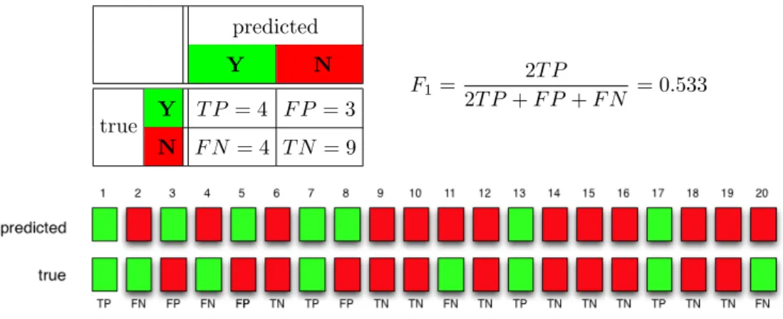
In order to see how human annotators may be effectively supported in their post-editing work, let us look at a specific example. Let us assume that the classifying task consists in deciding whether a given class applies or not to any of a set of unlabelled documents (binary case). Let us also assume that a set of unlabelled documents have been automatically classified; for simplicity of illustration we here assume that this set consists of 20 documents only. We can measure the accuracy obtained in this automatic classification job by (a) choosing an accuracy measure, (b) filling out a

(40)

CHAPTER 3. A RANKING METHOD FOR SATC predicted Y N true Y T P = 4 F P = 3 N F N= 4 T N = 9 F1= 2T P 2T P+F P +F N = 0.533

Figure 3.1: A worked-out example, representing a contingency table (upper left part of the figure) deriving from the automatically labelled examples (lower part) and from which accuracy is computed (upper right part).

contingency table, and (c) evaluating the chosen measure on this table. For illustration

purposes we assume that our accuracy measure is the well-known F1, described in

Chapter 2. Figure 3.1 depicts a situation in which the automatic classification process has returned 4 true positives, 3 false positives, 4 false negatives, and 9 true negatives, resulting in a value of F1 = ₍₂_·₄₎₊₃₊₄2·4 = 0.533. The 20 documents are represented in the two rows at the bottom via green and red cards; the upper row represents the classification decisions of the system (“predictions”), while the lower row represents the correct decisions that an ideal system would have taken. A green card represents a “yes” (the documents has the category), while a red card represents a “no” (the documents does not have the category); a correct decision is thus represented by the upper and lower card in the same column having the same colour.

Let us imagine a scenario in which the customer insists that the data must be clas-sified with an accuracy level of at leastF1= 0.800. In this case, after checking that the value ofF1that the automatic classifier has obtained is 0.533, the human annotator decides to validate some of the documents until the desired level of accuracy has been

obtained1_{. Let us assume that the coder examines the documents at the bottom of}

Figure 3.1 in left-to-right order. The first document that the annotator examines is a true positive; no correction needs to be done, the value ofF1 is unmodified, and the annotator moves on to the second document. This is a false negative, and

correct-ing it decreasesF N by 1 and increasesF P by 1, which means thatF1now becomes

F1=(2·5)+3+32·5 = 0.625. The third is a false positive, and correcting it decreasesF P by 1 and increasesT N by 1, which means thatF1 now becomesF1= ₍₂_·₅₎₊₂₊₃2·5 = 0.667.

1 _{Actually, the human annotator does} _not _{know the level of accuracy that the automatic}

classifier has obtained, since she does not know the true classification of documents. How-ever, this level of accuracy can be at leastestimated via ak-fold cross-validation.