Tree-based ensemble methods for predicting PV power generation and their comparison with support vector regression

(1)

Tree-based ensemble methods for predicting PV power generation

and their comparison with support vector regression

Muhammad Waseem Ahmad

*

, Monjur Mourshed, Yacine Rezgui

BRE Centre for Sustainable Engineering, School of Engineering, Cardiff University, Cardiff CF24 3AA, United Kingdom

a r t i c l e i n f o

Article history:

Received 13 April 2018 Received in revised form 24 August 2018 Accepted 28 August 2018 Available online 30 August 2018 Keywords:

Artiﬁcial intelligence Extremely randomised trees Random forest

Decision trees Ensemble algorithms Photovoltaic systems Prediction

Renewable energy systems

a b s t r a c t

The variability of renewable energy resources, due to the characteristic weatherfluctuations, introduces uncertainty in generation output that are greater than the conventional energy reserves the grid uses to deal with the relatively predictable uncertainties in demand. The high variability of renewable genera-tion makes forecasting critical for optimal balancing and dispatch of generagenera-tion plants in a smarter grid. The challenge is to improve the accuracy and the confidence level of forecasts at a reasonable compu-tational cost. Ensemble methods such as random forest (RF) and extra trees (ET) are well suited for predicting stochastic photovoltaic (PV) generation output as they reduce variance and bias by combining several machine learning techniques while improving the stability; i.e. generalisation capabilities. This paper investigated the accuracy, stability and computational cost of RF and ET for predicting hourly PV generation output, and compared their performance with support vector regression (SVR), a supervised machine learning technique. All developed models have comparable predictive power and are equally applicable for predicting hourly PV output. Despite their comparable predictive power, ET outperformed RF and SVR in terms of computational cost. The stability and algorithmic efficiency of ETs make them an ideal candidate for wider deployment in PV output forecasting.

1. Introduction

The projected global energy demand by 2050 will be approxi-mately 130 PWh or the equivalent of 1010tons of oil yearly [1,2]. The demand should be achieved without increasing global CO2 emis-sions level or relying only on the fossil-fuel based energy systems [3,4]. Developed and developing countries alike have initiated policies to raise the share of renewable energy in energy use as part of the global response to climate change. In March 2007, the EU set a target of 20% renewable energy by the year 2020. Photovoltaic systems will play a key role in mitigating climate change and meeting world's future energy demands. Solar energy is one of the most desirable sources of green energy because it is widely avail-able, clean, inexhaustible, safe and economically viable. The worldwide market of photovoltaic systems is increasing day by day due to the deterioration of the environmental conditions and depletion of conventional fossil-fuel based systems.

To tackle the challenge of mitigating climate change, power

systems' planning and operation will need to be performed ac-cording to the Smart-grid (SG) vision [5]. The vision aims at introducing and using new technologies and services to make electrical networks more reliable, secure, efﬁcient and eco-friendly [6]. Photovoltaic systems being one of the most clean and economically viable technologies, will play an important part to-wards the Smart-grid vision. Non-predictable renewable energy sources, e.g. photovoltaic system are being integrated into existing and new energy supply infrastructure. However, the stochastic nature of solar renewable energy introduces challenging issues for the optimal operation and control of SG systems. A balance, which is important for the secure operation of power systems, will need to be maintained between electricity production and consumption at any moment by continuously controlling demand and adjusting power generation capacity [7]. Predictive analytics will play a sig-niﬁcant role towards real-time optimal management of energy use, secure operation of power systems, and maintaining balance be-tween consumption and production.

According to Zamo et al. [8], solar energy prediction can be categorised intoﬁve types:

*Corresponding author.

E-mail addresses:[email protected](M.W. Ahmad),MourshedM@Cardiff. ac.uk(M. Mourshed),[email protected](Y. Rezgui).

Contents lists available atScienceDirect

Energy

j o u r n a l h o m e p a g e :w w w . e l s e v i e r . c o m / l o c a t e / e n e r g y

https://doi.org/10.1016/j.energy.2018.08.207

(2)

Intra-hourepredicting for next 15 min to 2 h with a time step of 1 min;

Hour-ahead _e predictions with hourly granularity with a maximum lookahead time of 6 h;

Day-aheadeone to three days ahead of hourly predictions; Medium-term_efrom 1 week to 2 months lead-time and daily

production; and

Long-term e predicting one to several years for monthly or annual production.

Each of this prediction category serves a different purpose. Intra-hour prediction is used for forecasting ramps and high-frequency changes in energy production. Day-ahead predictions are beneﬁcial in power system planning for unit commitment and dispatch, and for electricity trading [7]. Medium-term prediction is used for planning and asset management. Long-term predictions are useful for assessing resources and selecting potential renewable energy sites [8]. PV power output predictions are thus important to guarantee a balance between generation and demand with reduced capacity and cost of the operating reserves [9]. Producers can use power prediction for making decisions on the energy market, enabling them to minimise the impact of deviations between scheduled and actual power generation [5]. This will increase the revenues while reducing the penalties related to regulation costs [5,10]. Prosumers can use PV prediction models for planning their consumption patterns for matching on-site power generation and therefore maximising their proﬁts [11]. Predictive analytic tool, a core component of smart-grid, could be used for the following applications:

Optimal control of decentralised energy systems can be ach-ieved by using prediction model of renewable energy resources (RES), which allows grid operators, users, owner, etc. to make informed decisions (e.g. increasing share of RES, etc.)

Analysing performance characteristics of different solar PV systems.

Fault detection and diagnosis of PV systems by comparing actual and predicted performance. Prediction models can be used to automatically activate an alarm in case of any potential failure. In a recent article by Youssef et al. [12], the authors reviewed different artificial intelligence techniques used for PV systems. Most of the reviewed techniques require data available from PV systems for defining expert rules or developing models. These models are then used for sizing, control, predictions and fault detection and diagnosis. A recent article by Reynolds et al. [13] also provided an overview of different modelling techniques suitable for online or near real-time control applications. One of the main benefits of data-driven models is that they require less time to perform prediction and can be used for quick power system plan-ning decisions. One example of the above mentioned prediction applications is detailed in Ahmad et al. [14]. The authors used nonlinear autoregressive neural networks for predicting hourly solar irradiation. According to the authors, the developed models can be used to develop intelligent controllers that allow users to efficiently manage energy generated from solar PV and thermal systems. Decision trees are one of the most widely used data mining techniques, which uses a tree like structure to classify a set of data into various predefined target values. One of the key ad-vantages of decision tree-based methods is that the trained model can represent logical statements, which are easy to understand by a non-expert. In the review article by Youssef et al. [12], none of the cited work focussed on using decision tree-based ensemble methods for predicting PV power output; this shows that

ensemble-based methods (particularly decision tree-based

ensemble methods _e random forests, extremely randomised

trees, gradient boosted regression trees) are less explored. Random forests and extremely randomised trees are based on ensemble learning theory and have the ability to learn simple and complex problems [15]. They also require lessﬁne-tuning and often default hyper-parameters can result in better prediction capabilities.

1.1. Motivation and contributions

Accurate prediction of energy produced by PV systems has been identiﬁed as one of the key challenges of massive PV integrations [16]. It allows grid operators to manage electricity generation by making informed decisions, and hence, reduces cost and un-certainties. Improved prediction is also useful for participants in the electricity balancing market and energy managers, as they could avoid possible penalties incurred due to the discrepancies between predicted and produced energy [17]. Most widely used machine learning methods (e.g., artiﬁcial neural networks, support vector machines) have instability issues, and therefore are prone to be unreliable [18]. The instability could lead in large variations in the predicted values due to small changes in the input data [18,19]. As the model developed in this research could be used for real-time fault detection and diagnosis, and energy management, therefore, the stability of developed models is important. More advanced machine learning techniques, ensemble learning, were developed in the early 1990s to overcome these instability issues [19,20]. Ensemble-based techniques generally perform better than the in-dividual learners that construct them, as they overcome their limitations and there might not be enough data available to train a single model with better generalisation capabilities [21,22].

The research presented in this paper mainly addresses the following aspects.

The use of tree-based ensemble methods to provide insight into the analysis of the variable importance of each input feature. Currently, domain knowledge is widely used to reduce input variable space;

The use of ensemble-based techniques for solar PV systems as most of the previous research work are focussed on artiﬁcial neural networks and its variants, support vector machines and regressive methods, and;

To demonstrate that tree-based ensemble methods can improve the prediction and stability of the developed model. These techniques are more computationally efﬁcient as compared to the most widely use techniques in the literature (for example, support vector regression).

The paper compares the performance of a recently developed machine learning methodeextra trees, with random forest and support vector regression. The rest of the paper is organised as follows: Section2details literature review of techniques used for PV power generation prediction. In Section3, we describe princi-ples of random forest, extremely randomised trees and support vector regression. The methodology of the developed prediction models is presented in Section4. Prediction results and discussion are detailed in Section5, whereas concluding remarks and future research directions are presented at the end of the paper. 2. Related work

In literature, different forecasting techniques have been applied to predict photovoltaic (PV) power output. These studies can be classiﬁed as direct [23e26] and indirect [27e31] techniques. Direct methods are based on the system output, i.e. using historical PV outputs and weather data as inputs [32]. In indirect methods, soalr

(3)

radiation is predictedfirst by using its historical values and weather data. These predicted solar radiation values are then used to predict PV power output [32]. Hiyama and Kitabayashi [33] developed an artificial neural network based method to predict maximum power generation from a PV module. The authors used solar irradiation, outdoor air temperature and wind velocity as input features. From the results, it was found that the proposed method was able to provide better prediction results. In literature, similar studies were also performed by Bahgat et al. [34], Chen et al. [35], Rus-Casas et al. [36]. According to the authors of these studies, feedforward ANN is the most recommended artificial neural network, while the most important input features for predicting solar output are solar ra-diation and outdoor air temperature.

Almonacid et al. [37] proposed a methodology for short-term (1 h ahead) PV forecasting. The methodology was based on the accurate short-term forecast of the solar radiation and outdoor dry-bulb temperature. The authors developed two dynamic artificial neural networks for forecasting solar radiation and outdoor air temperature. These predicted values were then used to predict PV power. Sulaiman et al. [38] developed a hybrid multi-layer feed-forward neural network for predicting the output from a grid-connected PV system. The authors used an artificial immune sys-tem tofind optimal values of network's hyper-parameters. In this paper, a small number of data samples were used as training and testing datasets and therefore, the resulting model may not have captured seasonal variations. Kazem et al. [39] modelled solar PV power output by using support vector machines. The developed model used solar radiation and outdoor air temperature as inputs and predicted photovoltaic current. Kazem and Yousif [40] also used SVM and compared its performance against generalised feedforward networks (GFF), multilayer perceptron (MLP) and self-organising feature maps (SOFM). It was found that all developed models achieved a low value of RMSE of about 0.25.

Support vector machine technique can solve non-linear and high-dimensional problems. One of the key advantages of SVM is that they can overcome the problem of over-ﬁtting and have fewer chances of getting stuck in the local minima as it is a convex opti-mization algorithm [41]. Yang et al. [32] proposed a weather-based hybrid method for day-ahead hourly prediction of PV power output. The authors used self-organising map (SOM) and learning vector quantization (LVQ) networks for classifying the historical PV power output data. Support vector regressions (SVR) was then employed to train the input/output dataset, and fuzzy inference method was used to select an adequate trained model. It was found that the proposed method achieved better performance than the simple SVR and ANN. Shi et al. [26] also proposed PV prediction methodology based on weather classiﬁcation and support vector machines. The results showed that the proposed prediction model was effective and promising for grid-connected systems.

It is evident from the literature that different methodologies have been applied to predict photovoltaic power output. Artiﬁcial neural network is one of the most widely used methods. However, ANN requires the user to specify different parameters of the model (e.g. no. of hidden layer (s) neurons, number of neurons in hidden layers(s), no. of training epochs, etc.). Also, ANN has some limita-tions while dealing with highly uncertain data. On the other hand, fuzzy logic can not learn directly from historical data and may not be effective as it is based on human knowledge [42]. Generating expert rules for fuzzy logic systems is a challenging task, and therefore best practices or human knowledge is often used to develop initial rules. A review on probabilistic forecasting techniques for PV power generation can be found in van der Meer et al. [43].

Decision trees are one of most widely used machine learning techniques for classiﬁcation and regression problems. The method uses a tree-like structure to classify a set of data into various

prede_fined target values (for regression problems) [15]. However, traditional CART (classification and regression trees) have some limitations, e.g. thefinal tree is not guaranteed to be optimal, trees are unstable, and significant changes can occur due to a small change in the training sample values [15]. In order to overcome this drawback, different enhancements of CART were developed, e.g. random forest, extra trees, gradient boosted regression trees. To the best of authors' knowledge, there are limited studies that investi-gated the applicability of decision tree based method and in particular tree-based ensemble methods for predicting PV power generation. Zamo et al. [8] benchmarked prediction models for hourly PV electricity production. The authors compared ten ma-chine learning models, including binary regression trees, bagging, boosting, random forest and support vector machines. It was found that the RMSE was between 9% and 12% for different power plants. A recent article by Ref. [44] also explored the use of RF for pre-dicting output current of a photovoltaic grid-connected system. The RF model performed better than the ANN-based model. The paper presents ensemble-based machine learning techniques for pre-dicting 1-h-ahead prediction of PV power generation.

3. Machine learning techniques for PV forecasting 3.1. Support vector regression

Support vector regression have been extensively applied in building energy and renewable energy generation prediction ap-plications. The method is highly effective in solving non-linear problems even with small sample of training datasets. SVM adopts the structure risk minimisation (SRM) principle, which minimises an upper bound of the generalisation error comprising of the sum of the training error and a conﬁdence level [45]. This principle is different from the traditional empirical risk mini-misation (ERM), which only minimises the training error. The basic concept of SVM applied to regression problems is to introduce kernel function, map the input space into a higher dimensional feature spaces via a non-linear mapping and to perform a linear regression in this feature space [46,47].

Assuming normalised input parameters consists of a vectorXi andYiis the photovoltaic power output (irepresents theith data-point in the dataset). For this case, the sample set can be de_ﬁned asfðXi;YiÞgNi¼1, whereNis the total number of samples. Support vector regression approximate the function using the form given in Equation(1)[45,48].

Y¼fðXÞ ¼W$∅ðXÞ þb (1)

In Equation (1), ∅ðXÞ denotes the high-dimensional space. A regularised risk function, given in Equation(2), is used to estimate coefﬁcientsWandb[46].

Minimise:1 2kWk 2_þ_C1 N XN i¼1 LεðYi;fðXiÞÞ (2) LεðYi;fðXiÞÞ ¼ 0; jYifðXiÞj ε jYifðXiÞj ε; others (3) kWk2

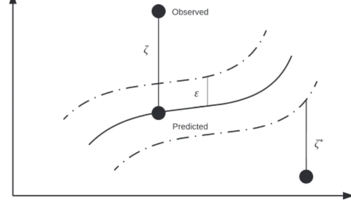
is known as regularised term andCis the penalty parameter to determine the trade-off between model ﬂatness and training error. The second term of Equation(2)is the empirical error and is measured by theε-intensity loss function (Equation(3)). This de-ﬁnes aεtube shown inFig. 1. The loss function is zero if the pre-dicted value is with the tube shown inFig. 1. Otherwise, the loss is the magnitude of the difference between the radiusεof the tube

(4)

and predicted value [46]. In order to estimate Wand b, above equation is transformed into the primal objective function given by Equation(4)[46].

z

1;

z

*1;W;b Minimise :1₂kWk2_þ_C1 N XN i¼1

z

1þ

z

*1 (4) Subject to: 8 < : YiW$∅ðxiÞ bεþ

z

1 W$∅ðxiÞ þbεþ

z

1;i¼1;2…;N

z

10

z

10

where,

z

1and

z

1are the slack variables. By introduction of kernel functionKðXi;XjÞ, the Equation(4)is written as bellow;

faig

a

* i Minimise :1₂XN i¼1 XN j¼1

a

i

a

*i

a

j

a

*j :KXi;Xj εXN i¼1

a

i

a

*i þXN i¼1 Yi

_a

i

a

*i (5) Subject to: 8 > < > : XN i¼1

a

i

a

i ¼0

a

i;

a

i2 0;C

In Equation (5),

a

i;

a

i are Lagrange multipliers, i and j are different samples. Therefore, Equation(1)becomes [46];

Y¼fðXÞ ¼XN i¼1

_a

i

a

i KX_i;X_jþb (6) 3.2. Random forest

A random forest (RF) is an ensemble-based machine learning technique, consisting of a large number of trees. In random forest, the performance of a number of weak learners (decision trees in this case) is boosted via a voting scheme. The main hallmarks of random forest are; 1) random feature selection, 2) bootstrap sam-pling, 3) out-of-bag (OOB) error estimation, and 4) full depth de-cision tree growing [51]. Random forest improves the classiﬁcation and regression trees (CART) by combining a large number of clas-siﬁcation and regression trees. In random forest, there is no need to

perform cross-validation as it can natively perform out-of-bag error estimation in the process of constructing the forest. The OOB error estimation is claimed to be unbiased in different tests [52].

The training procedure of a random forest can be summarised in following steps:

Draw a bootstrap sample from the original dataset;

For each bootstrap drawn in step 1, grow an unpruned regres-sion (or classiﬁcation) tree, with the following modiﬁcations: at each node, randomly sample (K) of the input variables and select the best split from among those variables; and

Repeat step 1 and 2 until C such trees as grown, and predict new data by aggregating the prediction of the C trees.

3.3. Extremely randomised regression trees

An extremely randomised trees (or extra trees) algorithm [53] is a tree-based ensemble machine learning method. It is a relatively recent algorithm and was developed as an extension of random forest algorithm. Extra trees algorithm uses a classical top-down procedure to build an ensemble of unpruned classiﬁ cation/regres-sion trees. Extra trees (ET) uses a random subset of features to train each base estimator, which is the same principle employed by random forest (RF) algorithm. However, instead of selecting the most discriminative split in each node, ET randomly selects the best feature along with the corresponding value for splitting the node [54]. Also, random forest uses bootstrap replica to train the pre-diction model, whereas, ET uses the whole training dataset to train each regression tree in the forest. These key differences make ET less likely to overﬁt a data as they have reported better perfor-mance in Ref. [53].

4. Methodology 4.1. Data description

The studied photovoltaic system has a peak power of 50 kWp and comprises of 200 modules with each having a capacity of 250 Wp. The system is installed in a low energy educational building (rated BREEAM excellentzLEED platinum). Power output from the system is metered every 30 min. The building also has an on-site weather station, which monitors solar radiation, outdoor air tem-perature and relative humidity, wind speed and direction, and at-mospheric pressure. The developed prediction models are deﬁned and trained to obtain best prediction results. For each trained model, the input dataset includes 1-h interval data of weather parameters, time information and previous hour solar PV power output values. The output of the model is the next hour PV power output from the system. The hourly values of outdoor air temper-ature, relative humidity, solar radiation and wind speed are shown inFig. 2.Fig. 3shows the system's hourly power output.

4.2. Model performance evaluation

To assess the performance of developed models, root mean square error (RMSE), mean absolute error (MAE) and determination coefficient (R2) were determined. Determination coefficient was adopted to measure the correlation between the actual and pre-dicted PV values. The former two indicators are defined as below;

RMSE¼ ffiffiffiffiffiffiffiffiffiffiffiffiffiffiffiffiffiffiffiffiffiffiffiffiffiffiffiffiffiffiffiffi PN i¼1ðyibyiÞ2 N s (7)

Fig. 1.The parameters of the support vector regression. Source: [49,50].

(5)

MAE¼1 N

XN i¼1

jbyiyij (8)

wherebyiis the predicted value,yiis the actual value, and N is the

total number of samples. In this work, root mean squared error (RMSE) is used as a primary evaluation metric. MAE is used as a_ﬁrst tie-breaker, and R2 is used as theﬁnal breaker. The two tie-breaker were taken in account when the primary evaluation metric (RMSE) did not provide a statistical difference between two models.

The implementation of extra trees, random forest, support vector regression included in the scikit-learn [55] module of python programming language was used for all developmental and experimental work. The work was carried out on a personal com-puter (Intel Core i5 2.50 GHz with 16 GB of RAM).

5. Prediction results and discussion

This section details the prediction results obtained with tree-based ensemble machine learning methods (random forest and extra trees) and support vector regression, which are described in Section3. This section also presents an assessment of the impact of different hyper-parameters on model's performance. For this pur-poses, a stepwise searching method to _ﬁnd optimal values of model's hyper-parameters.

5.1. ET and RF hyper-parametric tuning

Performance of studied ensemble tree-based algorithms de-pends on the adjustment of three-hyper-parameters, i.e. number of trees (M), number of minimum samples required for splitting a node (nmin) and attribute selection strength parameter (K).Kis the number of randomly selected features at each node during the tree growing process. It determines the strength of variable selection process and for most regression problems is set top, wherepis the dimension of the feature vector [53]. ParameterMdenotes the total number of trees in the forest, for this study weﬁxed this parameter to 1000 trees. It is worth mentioning that the number of trees is directly related to computational time, and therefore a reasonable number of trees needs to be selected to optimise prediction per-formance and computational time. For ET, different values ofnminin

Fig. 2.Weather data of Cardiff, Wales, UK. The data shown in theﬁgure is from 01/01/2015 00:00 until 31/12/2015 23:00.

Fig. 3.Actual hourly PV system power output. The data shown in theﬁgure is from 01/ 01/2015 00:00 until 31/12/2015 23:00.

Table 1

Results of variousnmin, whereK¼nandM¼1000 for ET model.

nmin R2₍₎ _{RMSE (kWh)} _{MAE (kWh)}

2 0.9221 2.2646 1.0281

3 0.9224 2.2605 1.0256

5 0.9234 2.2456 1.0190

7 0.9245 2.2301 1.0121

(6)

the range of [2,10] were experimented to assess the prediction performance dependence onnmin.Table 1details the performance of prediction models while varyingnmin. It was found that varying nmindid not yield a signiﬁcant improvement for photovoltaic po-wer prediction dataset. For this dataset, a value of 3 was selected as it resulted in slightly better performance than the default value of 2. The minimum number of samples required to split an internal node could be an important hyper-parameter depending on the problem. However, in our case, this parameter did not signiﬁcantly improve our result (as demonstrated in the ET parametric study) and therefore was kept as default (i.e. equal to 2) for RF models.

For ET, K values were varied in the range of [1,5] (i.e., total number of features selected for model construction process). Table 2 shows that the attribute selection parameter did not signiﬁcantly improve the performance and therefore a default value of 5 (i.e., total number of selected features) was selected for this problem.Table 3presents the results obtained by varyingKfor RF models; it was found that for predicting hourly photovoltaic power output, this parameter did not signiﬁcantly enhance the performance of RF models. Therefore, we selected K¼2 for our experiments as it performed slightly better than other values and the trained RF model had an R2value of 90.10.

Maximum tree depth was also varied to the study models' performance dependence on this parameter. Table 4 shows that maximum depth has a significant influence on ET model's mance. It was found that deeper trees resulted in better perfor-mance. A maximum depth of 1 resulted in an R2_{value of 0.729348} (under-fitted model). It was also found that for ET models, trees deeper than 7 did not perform significantly better as the perfor-mance metrics were approximately equal. Also, the perforperfor-mance of trees deeper than 12 levels started to deteriorate. The depth of a tree in the forest is implicitlyfixed bynmini.e., the smaller the value of minimum samples required for splitting a node, the deeper the tree.Table 5shows the effect of tree depth on the performance of a random forest. It was found that a random forest constructed with deeper trees resulted in better prediction accuracy. A maximum depth of 1 led to under-fitting, and the model resulted in a lower value of R2(0.729976) and higher values of MAE (3.752482) and RMSE (3.752482). Also, the performance of the model did not signi_ficantly improve with trees deeper than 7 levels. The results show that default values of hyper-parameters of studied ensemble tree-based models are near-optimal and could result in a robust prediction model.

5.2. SVR hyper-parametric tuning

Performance of support vector regression models depends on a) kernel function and b) speciﬁc parameters of the selected kernel function. In literature, radial-basis function (RBF) kernel is widely used for regression problems. It non-linearly maps samples into a higher dimensional space and can easily handle the non-linear relationship between class labels and attributes [49]. Polynomial kernel function has more hyper-parameter to tune as compared to RBF kernel, and as more parameters increase the complexity of the model, therefore RBF was selected as a preferred kernel function for

this problem. For RBF, there are three hyper-parameters to tune, i.e. kernel coefﬁcient (

g

), penalty parameter of the error term (C) and radius (ε).

According to the deﬁnition of kernel coefﬁcient by Chang and Lin [56],

g

¼1=K; where K is the number of input variables. Therefore, in this case,

g

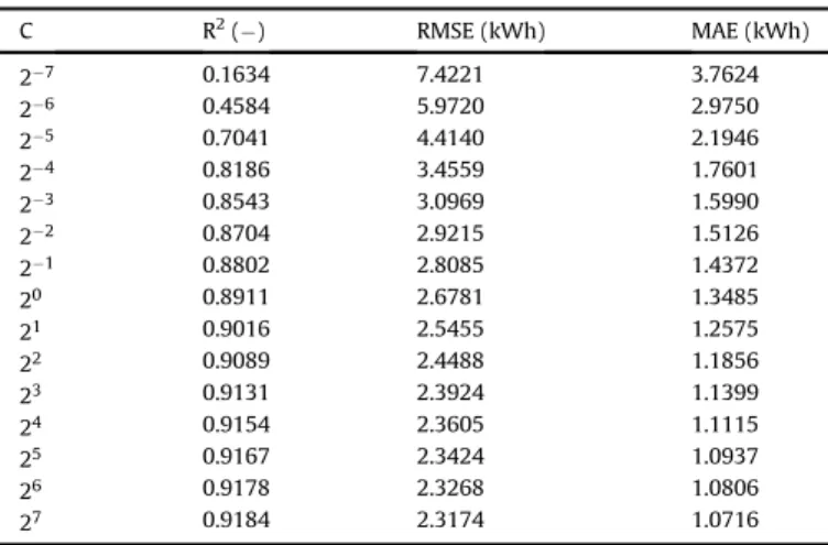
¼1/5 was used to estimate hourly PV power output values. Penalty parameter (C) is used tofind the trade-off between the model complexity and the degree to which deviations larger thanεare tolerated in the optimization formu-lation. A small value of C will place small weight on the training data and therefore result in under-fitted model [50]. On the other hand, too large values of C would under-fit the training dataset as the objective will only be to minimise the empirical risk only. A step-wise search was used tofind optimal values of C andε. In this study,εwasfixed at 0.1 while varying C over the range of 27_and 27_{. The results are shown in}_{Table 6}_{. From}_{Table 6}_{, it is evident that} initially there was significant increase in the performance of the model with an increase of C, however with larger values of C, the performance increased only slightly. It was also found that the larger values of C resulted in over-fitting the training dataset. It was concluded that higher values of C did not significantly enhance the model's performance and also it is computationally extensive to train SVR model with larger values of C. Therefore, a value of 23was selected for C. Parameterεcontrols the width of theε-intensive zone and a too large value of this parameter deteriorate the Table 2

Results of various K, wherenmin¼2 andM¼1000 for ET model.

K R2₍₎ _{RMSE (kWh)} _{MAE (kWh)} 1 0.9255 2.2148 1.0433 2 0.9258 2.2105 1.0164 3 0.9245 2.2300 1.0168 4 0.9226 2.2561 1.0242 5 0.9218 2.2685 1.0287 Table 3

Results of variousK, wherenmin¼2 andM¼1000 for RF model.

K R2₍₎ _{RMSE (kWh)} _{MAE (kWh)} 1 0.9260 2.2072 1.0202 2 0.9270 2.1923 0.9914 3 0.9257 2.2118 0.9959 4 0.9245 2.2291 0.9993 5 0.9239 2.2383 1.0019 Table 4

Results of variousdmin, wherenmin¼2,K¼5 andM¼1000 for ET model.

dmin R2₍₎ _{RMSE (kWh)} _{MAE (kWh)}

1 0.7293 4.2215 3.0193 3 0.8758 2.8598 1.6635 5 0.9122 2.4040 1.2384 7 0.9231 2.2499 1.0851 9 0.9258 2.2108 1.0326 10 0.9262 2.2043 1.0194 11 0.9261 2.2053 1.0126 12 0.9260 2.2080 1.0080 13 0.9251 2.2208 1.0109 15 0.9239 2.2381 1.0139 20 0.9220 2.2661 1.0273 Table 5

Results of variousdmin, wherenmin¼2,K¼5 andM¼1000 for RF model.

dmin R2₍₎ _{RMSE (kWh)} _{MAE (kWh)}

1 0.7300 4.2166 3.0440 3 0.8769 2.8470 1.6583 5 0.9122 2.4046 1.2348 7 0.9233 2.2470 1.0832 9 0.9266 2.1986 1.0244 10 0.9271 2.1903 1.0106 11 0.9272 2.1891 1.0007 12 0.9270 2.1919 0.9945 13 0.9265 2.1999 0.9922 15 0.9251 2.2201 0.9966 20 0.9237 2.2409 1.0028

(7)

accuracy of training dataset [49]. For tuningε, its values were varied over the range of 210_{and 2}3_{while keeping C}_¼_{8. From the results} inTable 7, it can be seen that smaller values ofεdid not have sig-niﬁcant inﬂuence on the performance of the model. However, the performance drastically reduced for values larger than 2. From re-sults, a value of 25_{was selected for}_ε_.

5.3. Testing results

Predictive performance of all of the three developed models are

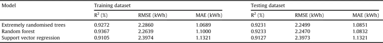
nearly comparable,Fig. 4illustrates the plots of hourly PV power output values predicted by RF model vs measured data for the testing dataset. The results clearly show the level of linear rela-tionship to illustrate the model's capability to accurately predict PV power output. Due to higher ﬂuctuations of solar radiation (and therefore in PV power output), more differences between actual and prediction values are observed during some of the hours in the testing dataset. Nevertheless, the developed models showed strong non-linear mapping generalisation ability, and can be effective in predicting hourly PV power output. A comparison between the measured and predicted values for both training and testing data-sets is given in Table 8. According to the results, RF performed marginally better on both training and testing datasets as compared to the other two developed models. For all three models, the R2values were higher than 90% and RMSE values were in the range of 2.24 and 2.40. From these results, it is evident that the developed models have capabilities to accurately predict the hourly PV power output.

A comparison of different computational intelligence models and actual PV data is presented inTable 9. The mean value, which measures the central tendency within a dataset, shows that all models closely resemble the actual PV data. Standard deviation quantify the amount of variations and it was found that SVM has nearly similar standard deviation as actual PV data. Median values of all three developed models do not match with the actual data. Minimum and maximum values assist in identifying outliers in the dataset. It was found that SVM has a slightly lower minimum value. Whereas, RF and ET have maximum values higher than the maximum value of the actual PV data. Skewness and Kurtosis measure the normality of a dataset. In other terms, Skewness and Kurtosis measure the“tailedness”and“asymmetry”of the proba-bility distribution of a real-valued random variable. It was found that the developed models have marginally different Skewness and Kurtosis values than the actual PV data's values.

5.4. Number of training samples

The number of samples in the training dataset has two impacts on machine learning model a) with the increase in the number of training data sample, it is expected that the prediction accuracy of the model will increase, and b) it increases the training time of the model and memory usage during the training phase. To demon-strate the effect of training data sample on model's performance and time required to construct a model, different experiments were performed by varying the number of samples in the training dataset.Fig. 5 (a)demonstrates the effect of the number of training data samples on prediction accuracy. Performance evaluation metric (R2) was calculated on training and testing datasets. For ET Table 6

Results of variousC, whereε¼0.1 for SVM model.

C R2₍₎ _{RMSE (kWh)} _{MAE (kWh)} 27 _0.1634 _7.4221 _3.7624 26 _0.4584 _5.9720 _2.9750 25 _0.7041 _4.4140 _2.1946 24 _0.8186 _3.4559 _1.7601 23 _0.8543 _3.0969 _1.5990 22 _0.8704 _2.9215 _1.5126 21 _0.8802 _2.8085 _1.4372 20 _0.8911 _2.6781 _1.3485 21 _0.9016 _2.5455 _1.2575 22 _0.9089 _2.4488 _1.1856 23 _0.9131 _2.3924 _1.1399 24 _0.9154 _2.3605 _1.1115 25 _0.9167 _2.3424 _1.0937 26 _0.9178 _2.3268 _1.0806 27 _0.9184 _2.3174 _1.0716 Table 7

Results of variousε, whereC¼23_{for SVM model.}

ε R2₍₎ _{RMSE (kWh)} _{MAE (kWh)} 210 _0.9127 _2.3980 _1.1310 29 _0.9127 _2.3982 _1.1310 28 _0.9126 _2.3984 _1.1312 27 _0.9126 _2.3983 _1.1312 26 _0.9126 _2.3981 _1.1315 25 _0.9127 _2.3974 _1.1320 24 _0.9129 _2.3951 _1.1340 23 _0.9131 _2.3915 _1.1456 22 _0.9132 _2.3899 _1.1745 21 0.9133 2.3890 1.2343 20 _0.9108 _2.4231 _1.4273 21 _0.8959 _2.6183 _1.8857 22 _0.8351 _3.2956 _2.7262 23 _0.6166 _5.0241 _4.3177

(8)

and RF, it was found that increasing the number of samples in-creases models' performance on the testing dataset. It can be seen inFig. 5(a) that both ET and RF showed almost same behaviour on the testing dataset, and models' accuracy quickly increased be-tween n¼250 and n¼1000. SVR showed relatively lower accuracy on both training and testing datasets.Fig. 5(b) shows that RF has signiﬁcantly higher training and prediction time as compared to ET and SVR. RF's training and prediction time has approximately direct relationship with the number of data samples. It can be noticed that ET has the lowest training and prediction time (8.46 s) than the other two techniques (14 s for SVR and 21.5 s for RF) on full sets of training and testing datasets. As discussed by Ahmad et al. [15], it is also worth mentioning that training time could depend on a number of factors. e.g. implementation of the studied algorithm, input data representation and sparsity, complexity of the model (e.g. increasing number of trees could increase the complexity of the problem and also the training time) and feature extraction.

Fig. 6shows the relative importance of each input feature used during the training phase of ensemble tree-based algorithms as well as its Pearson correlation with PV output. It is interesting to note that each of the tested machine learning models has different variable importance score for each input feature. As an example; for the ET model, solar radiation is the most inﬂuential input feature with a variable importance score of 0.782. On the other hand, the

previous hourly value of PV output is the most important param-eter for the RF model. Both of these input features (i.e. solar radi-ation and previous hour value) are highly correlated to PV power output, as demonstrated by their Pearson correlation coefﬁcients. It can also be noticed that month of the year, the day of the week and outdoor air relative humidity are negatively related to the PV power output. It is worth mentioning that the procedure of selecting important variables was performed before training ET and RF models, and only inﬂuential variables were used for model devel-opment purposes. Evaluating feature importance helps in dimen-sionality reduction to improve model's performance on a high-dimensional dataset. The performance by reducing dimension of input features can be enhanced by enhancing the generalisation capabilities of the model and/or reducing the training time [15]. Table 10illustrates the R2, RMSE and MAE values for both training and testing datasets by using all or some of the considered input variables for the ET model. First, the performance metrics are shown for a model which considers all of the input variables and then metrics are listed for the ET model considering fewer inputs. Table 8

Comparison of models on training and testing datasets.

Model Training dataset Testing dataset

R2_(%) _{RMSE (kWh)} _{MAE (kWh)} _R2_(%) _{RMSE (kWh)} _{MAE (kWh)}

Extremely randomised trees 0.9272 2.2860 1.0689 0.9231 2.2499 1.0851

Random forest 0.9367 2.2639 1.1000 0.9233 2.2470 1.0832

Support vector regression 0.9105 2.3974 1.1321 0.9127 2.3973 1.1321

Table 9

Comparison of the statistical measures on testing dataset for different studied ma-chine learning models.

Factor/variable Actual PV data RF ET SVM

Mean 4.594 4.900 4.901 4.854 Median 0.066 0.247 0.276 0.277 Standard Deviation 7.980 7.824 7.842 7.986 Sample Variance 63.674 61.221 61.505 63.776 Kurtosis 3.654 2.426 2.427 2.982 Skewness 2.049 1.775 1.777 1.903 Range 39.880 35.262 35.320 39.567 Minimum 0 0.005 0.006 0.168 Maximum 39.880 35.267 35.326 39.399 Sum 15577.164 16617.252 16617.966 16460.067

Fig. 5.a) Effect of number of training data samples on prediction accuracy, b) Effect of number of training data samples on training and prediction time.

Fig. 6.Feature importance and Pearson correlation for PV power output prediction. Notes: Previous: Previous hour's PV power output, Mon: Month of the year, Day: Day of the year, Hr: Hour of the day, PR: Atmospheric pressure, WS: Wind speed, Rad: Solar radiation, RH: Outdoor air relative humidity, DBT: outdoor air dry-bulb temperature.

(9)

Please note that all models are trained and tested on the same datasets. From results, it is clear that even if solar radiation and previous hour energy generation are the most inﬂuential variables (see results inFig. 6), using only them deteriorates the performance of the model. Therefore, it is critical to use other important vari-ables selected by the RF and ET algorithms.

6. Conclusions

In this study, the feasibility of utilizing tree-based ensemble methods (extra trees and random forests) and support vector regression to predict the hourly output from a photovoltaic system was evaluated. For this purpose, a PV system installed in Cardiff, UK was used as a case study. The capability of decision tree-based ensemble for predicting the photovoltaic power produced has been veriﬁed with a better prediction accuracy of the models. To appraise the models' prediction performance, different well-known statistical parameters of MAE, RMSE and R2were used. It has been found that ET and RF performed marginally better than the widely used machine learning methodesupport vector regression. The results also demonstrated that ET has signi_ﬁcantly lower training and prediction time, i.e. 8.46 s as compared to 21.5 s and 1 s for RF and SVR, respectively. The paper also proposed using tree-based ensemble methods to provide insight into the analysis of the importance of each input variable. The presented analysis will allow researchers and industry practitioners to gain better under-standing of the modelled systems.

The developed machine learning models can be applied to predict 1-h-ahead PV power generation based on different weather parameters, date time information and previous hour values of photovoltaic power output. The models are developed for stand-alone PV system; however, they could be used to predict PV po-wer output in grid-connected systems. The advantages of the tree-based ensemble methods are that they have only a few tuning parameters and in most cases default hyper-parameter can result in satisfactory prediction performance. RF performs internal cross-validation (i.e., using out-of-bag samples) and can be used to handle high-dimensional datasets. The proposed extra trees algo-rithm is computationally efﬁcient and is more suitable for online or near real-time optimization/control applications. In future, the designed ensemble-based models will be used to detect perfor-mance gap in the PV system, and the system will be able to detect faults based on the comparison between actual and predicted po-wer output. There will be a need to incorporate a procedure to detect different types of PV faults. There is also a need to investigate the performance of other decision tree-based methods, e.g.,

Gradient boosted regression trees, Mondrian forests. Future studies will also focus on assessing the performance of tree-based ensemble methods in other time-scales and for different climate conditions. Development of separate models based on weather classiﬁcation (i.e., classifying weather on different weather condi-tions_eclear sky, foggy day, cloudy day and rainy day) will also be investigated in future. There is also a need to explore Big Data technologies for training and deploying renewable energy predic-tion models.

Acknowledgement

The work was carried out in the framework of the FP7 project (Grant reference e 609154) PERFORMER “Portable, Exhaustive, Reliable, Flexible and Optimised approach to Monitoring and Evaluation of building energy performance” and Horizon 2020 project (Grant referencee731125) PENTAGON“Unlocking Euro-pean grid local ﬂexibility trough augmented energy conversion capabilities at district-level”. The authors acknowledge theﬁ nan-cial support from the European Commission.

References

[1] International energy agency, ey world energy statistics. IEA; 2011.http:// www.iea.org/publications/freepublications/publication/key_world_energy_ stats-1.pdf,2011.

[2] Lewis NS. Powering the planet. MRS Bull 2007;32(10):808e20.

[3] Ahmad MW, Mourshed M, Mundow D, Sisinni M, Rezgui Y. Building energy metering and environmental monitoringea state-of-the-art review and di-rections for future research. Energy Build 2016a;120(Supplement C):85e102. ISSN 0378-7788,https://doi.org/10.1016/j.enbuild.2016.03.059.

[4] Larcher D, Tarascon J-M. Towards greener and more sustainable batteries for electrical energy storage. Nat Chem 2015;7(1):19e29.

[5] Bracale A, Caramia P, Carpinelli G, Di Fazio AR, Ferruzzi G. A Bayesian method for short-term probabilistic forecasting of photovoltaic generation in smart grid operation and control. Energies 2013;6(2):733e47.

[6] Bouhafs F, Mackay M, Merabti M. Links to the future: communication re-quirements and challenges in the smart grid. IEEE Power Energy Mag 2012;10(1):24e32. https://doi.org/10.1109/MPE.2011.943134. ISSN 1540-7977.

[7] Foley AM, Leahy PG, Marvuglia A, McKeogh EJ. Current methods and advances in forecasting of wind power generation. Renew Energy 2012;37(1):1e8. ISSN 0960-1481,https://doi.org/10.1016/j.renene.2011.05.033.

[8] Zamo M, Mestre O, Arbogast P, Pannekoucke O. A benchmark of statistical regression methods for short-term forecasting of photovoltaic electricity production, part I: deterministic forecast of hourly production. Sol Energy 2014;105(Supplement C):792e803. ISSN 0038-092X, http://www. sciencedirect.com/science/article/pii/S0038092X13005239.

[9] Potter CW, Archambault A, Westrick K. Building a smarter smart grid through better renewable energy information. In: IEEE/PES power systems conference and exposition; 2009. p. 1e5. https://doi.org/10.1109/PSCE.2009.4840110, 2009.

[10] Pinson P, Chevallier C, Kariniotakis GN. Trading wind generation from short-term probabilistic forecasts of wind power. IEEE Trans Power Syst 2007;22(3): Table 10

Comparison of full and reduce ET models on training and testing datasets.

Input variables Training dataset Testing dataset

R2_(%) _{RMSE (kWh)} _{MAE (kWh)} _R2_(%) _{RMSE (kWh)} _{MAE (kWh)} DBT, RH, Rad, WS, PR, Hour, Day, Mon, Previous 0.9192 2.3348 1.2056 0.9156 2.3574 1.2197

RH, Rad, WS, PR, Hr, Day, Mon, Previous 0.9209 2.3092 1.1706 0.9178 2.3262 1.1812

DBT, Rad, WS, PR, Hr, Day, Mon, Previous 0.9212 2.3052 1.1672 0.9181 2.3216 1.1779

DBT, RH, WS, PR, Hr, Day, Mon, Previous 0.8926 2.6912 1.4912 0.8858 2.7426 1.5396

DBT, RH, Rad, PR, Hr, Day, Mon, Previous 0.9214 2.3017 1.1669 0.9184 2.3180 1.1789 DBT, RH, Rad, WS, Hr, Day, Mon, Previous 0.9212 2.3058 1.1652 0.9182 2.3206 1.1748 DBT, RH, Rad, WS, PR, Day, Mon, Previous 0.8964 2.6433 1.4065 0.8862 2.7376 1.4591

DBT, RH, Rad, WS, PR, Hr, Mon, Previous 0.9210 2.3087 1.1698 0.9180 2.3231 1.1793

DBT, RH, Rad, WS, PR, Hr, Day, Previous 0.9211 2.3065 1.1731 0.9179 2.3258 1.1841

Temp, RH, Rad, WS, PR, Hr, Day, Mon 0.8851 2.784 1.4212 0.8801 2.8094 1.4544

Radiation 0.8450 3.2327 1.5878 0.8367 3.279 1.6390

Previous 0.83540 3.3317 1.8569 0.8199 3.4436 1.9453

Notes: DBT: Outdoor air temperature, RH: Relative humidity, Rad: Solar radiation, hr: Hour of the day, WS: Wind speed, Day: Day of the year, Previous: Previous hour's PV power output, PR: Atmospheric pressure, Month: Month of the year.

(10)

1148e56.https://doi.org/10.1109/TPWRS.2007.901117. ISSN 0885-8950. [11] Sharma N, Sharma P, Irwin D, Shenoy P. Predicting solar generation from

weather forecasts using machine learning. In: IEEE international conference on smart grid communications (SmartGridComm); 2011. p. 528e33.https:// doi.org/10.1109/SmartGridComm.2011.6102379, 2011.

[12] Youssef A, El-Telbany M, Zekry A. The role of artiﬁcial intelligence in photo-voltaic systems design and control: a review. Renew Sustain Energy Rev 2017;78:72e9.

[13] Reynolds J, Ahmad MW, Rezgui Y. Holistic modelling techniques for the operational optimisation of multi-vector energy systems. Energy Build 2018;169:397e416. ISSN 0378-7788,http://www.sciencedirect.com/science/ article/pii/S0378778817340240.

[14] Ahmad A, Anderson T, Lie T. Hourly global solar irradiation forecasting for New Zealand. Sol Energy 2015;122:1398e408. ISSN 0038-092X,http://www. sciencedirect.com/science/article/pii/S0038092X15006118.

[15] Ahmad MW, Mourshed M, Rezgui Y. Trees vs Neurons: comparison between random forest and ANN for high-resolution prediction of building energy consumption. Energy Build 2017;147(Supplement C):77e89. ISSN 0378-7788,

https://doi.org/10.1016/j.enbuild.2017.04.038.

[16] E. P. I. Association, et al., Connecting the Sun: solar photovoltaics on the road to large-scale grid integration, [Brussels, Belgium] .

[17] Antonanzas J, Osorio N, Escobar R, Urraca R, de Pison FM, Antonanzas-Torres F. Review of photovoltaic power forecasting. Sol Energy 2016;136:78e111. ISSN 0038-092X, http://www.sciencedirect.com/science/article/pii/ S0038092X1630250X.

[18] Breiman L, et al. Heuristics of instability and stabilization in model selection. Ann Stat 1996;24(6):2350e83.

[19] Wang Z, Wang Y, Zeng R, Srinivasan RS, Ahrentzen S. Random Forest based hourly building energy prediction. Energy Build 2018;171:11e25.https:// doi.org/10.1016/j.enbuild.2018.04.008. ISSN 0378-7788.

[20] Hansen LK, Salamon P. Neural network ensembles. IEEE Trans Pattern Anal Mach Intell 1990;12(10):993e1001.

[21] Dietterich TG. Ensemble methods in machine learning. In: International workshop on multiple classiﬁer systems. Springer; 2000. p. 1e15. [22] Fan C, Xiao F, Wang S. Development of prediction models for next-day

building energy consumption and peak power demand using data mining techniques. Appl Energy 2014;127:1e10. https://doi.org/10.1016/j.ape-nergy.2014.04.016. ISSN 0306-2619.

[23] Wang S, Zhang N, Zhao Y, Zhan J. Photovoltaic system power forecasting based on combined grey model and BP neural network. In: International conference on electrical and control engineering; 2011. p. 4623e6.https:// doi.org/10.1109/ICECENG.2011.6057634, 2011.

[24] Li R, Li G-m. Photovoltaic power generation output forecasting based on support vector machine regression technique. Electr power 2008;2:031. [25] Yu T-C, Chang H-T. The forecast of the electrical energy generated by

photovoltaic systems using neural network method. In: International con-ference on electric information and control engineering; 2011. p. 2758e61.

https://doi.org/10.1109/ICEICE.2011.5778257, 2011.

[26] Shi J, Lee WJ, Liu Y, Yang Y, Wang P. Forecasting power output of photovoltaic systems based on weather classiﬁcation and support vector machines. IEEE Trans Ind Appl 2012;48(3):1064e9. https://doi.org/10.1109/ TIA.2012.2190816. ISSN 0093-9994.

[27] Yona A, Senjyu T, Saber AY, Funabashi T, Sekine H, Kim CH. Application of neural network to one-day-ahead 24 hours generating power forecasting for photovoltaic system. In: International conference on intelligent systems ap-plications to power systems; 2007. p. 1e6. https://doi.org/10.1109/ ISAP.2007.4441657, 2007.

[28] Capizzi G, Napoli C, Bonanno F. Innovative second-generation wavelets con-struction with recurrent neural networks for solar radiation forecasting. IEEE Trans Neural Network Learn Syst 2012;23(11):1805e15. https://doi.org/ 10.1109/TNNLS.2012.2216546. ISSN 2162-237X.

[29] Cao S, Weng W, Chen J, Liu W, Yu G, Cao J. Forecast of solar irradiance using chaos optimization neural networks. In: Asia-paciﬁc power and energy en-gineering conference; 2009. p. 1e4. https://doi.org/10.1109/ APPEEC.2009.4918387, 2009. ISSN 2157-4839.

[30] Zhang P, Takano H, Murata J. Daily solar radiation prediction based on wavelet analysis. In: SICE annual conference 2011, ISSN pending; 2011. p. 712e7. [31] Tanaka K, Uchida K, Ogimi K, Goya T, Yona A, Senjyu T, Funabashi T, Kim CH.

Optimal operation by controllable loads based on smart grid topology considering insolation forecasted error. IEEE Trans Smart Grid 2011;2(3): 438e44.https://doi.org/10.1109/TSG.2011.2158563. ISSN 1949-3053. [32] Yang HT, Huang CM, Huang YC, Pai YS. A weather-based hybrid method for

1-day ahead hourly forecasting of PV power output. IEEE Trans Sustain Energy 2014;5(3):917e26. https://doi.org/10.1109/TSTE.2014.2313600. ISSN

1949-3029.

[33] Hiyama T, Kitabayashi K. Neural network based estimation of maximum po-wer generation from PV module using environmental information. IEEE Trans Energy Convers 1997;12(3):241e7.https://doi.org/10.1109/60.629709. ISSN 0885-8969.

[34] Bahgat A, Helwa N, Ahmad G, Shenawy EE. Maximum power point traking controller for PV systems using neural networks. Renew Energy 2005;30(8): 1257e68. ISSN 0960-1481,https://doi.org/10.1016/j.renene.2004.09.011. [35] Chen Y, Yang B, Dong J, Abraham A. Time-series forecasting usingﬂexible

neural tree model. Inf Sci 2005;174(3):219e35.

[36] Rus-Casas C, Aguilar J, Rodrigo P, Almonacid F, Perez-Higueras P. Classi ﬁcation of methods for annual energy harvesting calculations of photovoltaic gener-ators. Energy Convers Manag 2014;78:527e36.

[37] Almonacid F, PA~lrez-Higueras P, FernAndez EF, Hontoria L. A methodology~ based on dynamic artiﬁcial neural network for short-term forecasting of the power output of a PV generator. Energy Convers Manag 2014;85(Supplement C):389e98. ISSN 0196-8904, https://doi.org/10.1016/j.enconman.2014.05. 090.

[38] Sulaiman SI, Rahman TKA, Musirin I, Shaari S. An artiﬁcial immune-based hybrid multi-layer feedforward neural network for predicting grid-connected photovoltaic system output. Energy Procedia 2012;14(Supple-ment C):260e4. ISSN 1876-6102, http://www.sciencedirect.com/science/ article/pii/S1876610211043438. 2011 2nd International Conference on Ad-vances in Energy Engineering (ICAEE).

[39] Kazem HA, Yousif JH, Chaichan MT. Modeling of daily solar energy system prediction using support vector machine for Oman. Int J Appl Eng Res 2016;11(20):10166e72.

[40] Kazem HA, Yousif JH. Comparison of prediction methods of photovoltaic po-wer system production using a measured dataset. Energy Convers Manag 2017;148(Supplement C):1070e81. ISSN 0196-8904, http://www. sciencedirect.com/science/article/pii/S0196890417306027.

[41] Fortuna J, Capson D. Improved support vector classiﬁcation using PCA and ICA feature space modiﬁcation. Pattern Recogn 2004;37(6):1117e29.

[42] Ahmad MW, Mourshed M, Yuce B, Rezgui Y. Computational intelligence techniques for HVAC systems: a review. Build Simulat 2016b;9(4):359e98.

https://doi.org/10.1007/s12273-016-0285-4.

[43] van der Meer D, WidA~ln J, Munkhammar J. Review on probabilistic forecasting of photovoltaic power production and electricity consumption. Renew Sustain Energy Rev 2018;81:1484e512. ISSN 1364-0321,http://www.sciencedirect. com/science/article/pii/S1364032117308523.

[44] Ibrahim IA, Khatib T, Mohamed A, Elmenreich W. Modeling of the output current of a photovoltaic grid-connected system using random forests tech-nique. Energy Explor Exploit 2017:1. https://doi.org/10.1177/ 0144598717723648.https://doi.org/10.1177/0144598717723648.

[45] Dong B, Cao C, Lee SE. Applying support vector machines to predict building energy consumption in tropical region. Energy Build 2005a;37(5):545e53. ISSN 0378-7788,https://doi.org/10.1016/j.enbuild.2004.09.009.

[46] Li Q, Meng Q, Cai J, Yoshino H, Mochida A. Applying support vector machine to predict hourly cooling load in the building. Appl Energy 2009a;86(10): 2249e56. ISSN 0306-2619,https://doi.org/10.1016/j.apenergy.2008.11.035. [47] Vapnik V. The nature of statistical learning theory. Springer science&business

media; 2013.

[48] Lin J-Y, Cheng C-T, Chau K-W. Using support vector machines for long-term discharge prediction. Hydrol Sci J 2006;51(4):599e612. https://doi.org/ 10.1623/hysj.51.4.599.

[49] Dong B, Cao C, Lee SE. Applying support vector machines to predict building energy consumption in tropical region. Energy Build 2005b;37(5):545e53. [50] Li Q, Meng Q, Cai J, Yoshino H, Mochida A. Applying support vector machine to

predict hourly cooling load in the building. Appl Energy 2009b;86(10): 2249e56.

[51] Jiang R, Tang W, Wu X, Fu W. A random forest approach to the detection of epistatic interactions in case-control studies. BMC Bioinf 2009;10(1):S65. [52] Breiman L. Random forests. Mach Learn 2001;45(1):5e32.

[53] Geurts P, Ernst D, Wehenkel L. Extremely randomized trees. Mach Learn 2006;63(1):3e42.

[54] V. John, Z. Liu, C. Guo, S. Mita, K. Kidono, Real-time lane estimation using deep features and extra trees regression, Springer International Publishing, Cham, 721e733, doi:10.1007/978-3-319-29451-3_57, 2016.

[55] Pedregosa F, Varoquaux G, Gramfort A, Michel V, Thirion B, Grisel O, Blondel M, Prettenhofer P, Weiss R, Dubourg V, et al. Scikit-learn: machine learning in Python. J Mach Learn Res 2011;12(Oct):2825e30.

[56] Chang C-C, Lin C-J. LIBSVM: a library for support vector machines. ACM Trans Intell Syst Technol (TIST) 2011;2(3):27.