NBER WORKING PAPER SERIES
NEOCLASSICAL FACTORS
Long Chen
Lu Zhang
Working Paper 13282
http://www.nber.org/papers/w13282
NATIONAL BUREAU OF ECONOMIC RESEARCH
1050 Massachusetts Avenue
Cambridge, MA 02138
July 2007
For helpful discussions, we thank Sreedhar Bharath, Gerald Garvey (BGI discussant), Tyler Shumway,
Motohiro Yogo (UBC discussant), Richard Sloan, Scott Richardson, and seminar participants at Barclays
Global Investors, Hong Kong University of Science and Technology, UBC PH&N Summer Finance
Conference in 2007, and University of Michigan. Cynthia Jin provided valuable assistance in early
stages of this project. The views expressed herein are those of the author(s) and do not necessarily
reflect the views of the National Bureau of Economic Research.
Neoclassical Factors
Long Chen and Lu Zhang
NBER Working Paper No. 13282
July 2007
JEL No. G11,G12,G14,G24,G31,G32
ABSTRACT
Building on neoclassical reasoning, we propose a new multi-factor model that consists of the market
factor and factor mimicking portfolios based on investment and productivity. The neo- classical three-factor
model outperforms traditional factor models in explaining the average returns across testing portfolios
formed on momentum, financial distress, investment, profitability, accruals, net stock issues, earnings
surprises, and asset growth. Most intriguingly, winners have higher loadings than losers on both the
low-minus-high investment factor and the high- minus-low productivity factor, which in turn help
explain momentum profits.
Long Chen
321 Eppley
Department of Finance
The Eli Broad Graduate School of Management
Michigan State University
East Lansing
MI 48824
[email protected]
Lu Zhang
Finance Department
Stephen M. Ross School of Business
University of Michigan
701 Tappan Street, ER 7605 Bus Ad
Ann Arbor MI, 48109-1234
and NBER
1
Introduction
The Sharpe (1964) and Lintner (1965) capital asset pricing model (CAPM) cannot explain many anomalies. For example, DeBondt and Thaler (1985), Fama and French (1992), and Lakonishok, Shleifer, and Vishny (1994) show that average returns covary with book-to-market, earnings-to-price, and long-term prior returns. Jegadeesh and Titman (1993) show that stocks with higher short-term prior returns earn higher average returns. Fama and French (1993, 1996) show that their three-factor model, which includes the market excess return (M KT), a mimicking portfolio based on market equity (SM B), and a mimicking portfolio based on book-to-market (HM L), can explain many CAPM anomalies. These include average returns across portfolios formed on size and book-to-market, earnings-to-price, cash flow-to-price, and long-term prior returns. Notably, these portfolios display strong HM L-loading variations in the same direction as their average returns.
However, the influential Fama-French (1993) three-factor model leaves important anomalies unexplained. Most glaringly, Fama and French (1996) show that their model cannot explain Je-gadeesh and Titman’s (1993) momentum profits. Winners load positively onHM Land losers load negatively on HM L. This pattern goes in the opposite direction as the average returns, leading the Fama-French model to exacerbate the momentum anomaly.
The relation between financial distress and average returns also eludes the Fama-French (1993) model. Fama and French (1996) conjecture that the averageHM Lreturn might be a risk premium for the relative distress of value firms. The returns of distressed firms tend to move together, mean-ing that their distress risk cannot be diversified and needs to be compensated with a risk premium. However, recent studies show that the distress risk is associated with lower average returns (e.g., Dichev 1998, Griffin and Lemmon 2002, Campbell, Hilscher, and Szilagyi 2007). Using a compre-hensive measure of financial distress, Campbell et al. report that more distressed stocks earn lower average returns despite their higher total volatilities, market betas, andSM B- andHM L-loadings.1 We show that the momentum and the distress anomalies are related, and are captured by a new multi-factor model motivated from neoclassical reasoning. The model says that the expected return on a portfolio in excess of the risk-free rate,E[Rj]−Rf, is described by the sensitivity of its return to three factors: M KT, the difference between the return on a portfolio of low investment-to-assets stocks and the return on a portfolio of high investment-to-assets stocks (IN V), and the difference
1
Campbell, Hilscher, and Szilagyi (2007) conclude that: “This result is a significant challenge to the conjecture that the value and size effects are proxies for a financial distress premium. More generally, it is a challenge to standard mod-els of rational asset pricing in which the structure of the economy is stable and well understood by investors (p. 29).”
between the return on a portfolio of high earnings-to-assets stocks and the return on a portfolio of low earnings-to-assets stocks (P ROD). Specifically, the expected excess return on portfolio j is:
E[Rj]−Rf =bjE[M KT] +ijE[IN V] +pjE[P ROD] (1) in whichE[M KT], E[IN V], andE[P ROD] are expected premiums, and the factor loadings,bj, ij, and pj are the slopes in the time series regression:
Rj−Rf =aj+bjM KT +ijIN V +pjP ROD+εj (2)
In our 1972–2006 sample,IN V andP RODearn average returns of 0.34% (t= 4.15) and 0.73% per month (t = 5.67), respectively. These average returns subsist after adjusting for their expo-sures to traditional factors such as the Fama-French (1993) factors and the Carhart (1997) factors. We find that the neoclassical three-factor model goes a long way in describing the cross section of average returns on NYSE, Amex, and NASDAQ stocks.
Most important, the neoclassical model outperforms the Fama-French (1993) model in explain-ing the average returns of 25 size and momentum portfolios. Usexplain-ing the six-month momentum definition of Jegadeesh and Titman (1993), we find that none of the winner-minus-loser portfolios across five size quintiles have significant alphas. The alphas, ranging from −0.02% to 0.34% per
month, are all within 1.6 standard errors of zero. For comparison, the five winner-minus-loser alphas vary from 0.64% (t = 2.77) to 1.02% per month (t = 6.04) in the CAPM and from 0.75% (t = 2.92) to 1.14% per month (t = 6.07) in the Fama-French model. In total, seven out of the 25 size and momentum portfolios have significant neoclassical alphas, and our model is rejected by the Gibbons, Ross, and Shanken (1989, GRS) test. However, the number of significant alphas is about half of that in the CAPM (13) and that in the Fama-French model (13).
One reason for the relative success of the neoclassical model is that winners have higherP ROD -loadings than losers, meaning that winners are more profitable than losers. More intriguingly, win-ners also have higher IN V-loadings than losers. The crux is timing. We show that winners (with high valuation ratios) indeed invest more than losers (with low valuation ratios) at the portfolio formation month t. But more important, winners invest less than losers in the event time before montht−8 ort−12, depending on the specific size quintile. Because IN V is rebalanced annually,
the higher IN V-loadings for winners accurately reflect their lower investment than losers several quarters prior to the monthly portfolio formation.
The neoclassical model fully captures the negative relation between financial distress and aver-age returns. The high-minus-low distress decile earns a neoclassical alpha of 0.18% per month (t= 0.83). And the model cannot be rejected using distress deciles by the GRS test (p-value = 0.08). In contrast, the corresponding alpha is−1.23% (t=−4.15) in the CAPM and−1.34% (t=−5.22)
in the Fama-French (1993) model. And both models are rejected by the GRS test at the 1% level. The P ROD-loading is the main driver of our model performance: More distressed firms are less profitable and have lowerP ROD-loadings than less distressed firms. Previous studies overlook the productivity-return relation, and, not surprisingly, find the distress-return relation anomalous.
Since Fama and French (1996), several other anomaly variables have received much attention, including earnings surprises, investment, profitability, accruals, net stock issues, and asset growth. (We provide detailed references later in this section and in Section 2.) We show that the neoclassi-cal model outperforms traditional factor models in explaining these anomalies, sometimes by a big margin. For example, in the universe of 25 investment and profitability portfolios, the neoclassical alphas for the five high-minus-low investment portfolios are all within 1.5 standard errors of zero. The alpha with the highest magnitude is−0.30% per month (t=−1.45) in the lowest-profitability
quintile. In contrast, the corresponding alpha is −1.01% (t= −4.67) in the CAPM and −0.70%
(t =−3.45) in the Fama-French model. Further, the high-minus-low profitability portfolio in the
highest-investment quintile earns a neoclassical alpha of 0.27% (t= 1.34), whereas the correspond-ing alpha is 1.22% (t= 4.96) in the CAPM and 1.43% (t= 6.08) in the Fama-French model.
However, our neoclassical model underperforms the Fama-French (1993) model in explaining the anomalies formed on valuation ratios such as book-to-market (B/M). While the Fama-French model explains these anomalies through theirHM Lfactor, the main driver in our model is theIN V factor. Stocks with higher valuation ratios invest less, load more on the low-minus-highIN V factor, and earn higher average returns. But empirically, the explanatory power of IN V for valuation-sorted portfolio returns is not as high as that of HM L. This evidence lends support to Fama and French (2007), who show that including net stock issues and asset growth in cross-sectional regressions has little impact on the book-to-market effect. However, the small-growth portfolio only earns a tiny neoclassical alpha of−0.03% per month (t=−0.10) in contrast to the CAPM alpha
of −0.63% (t=−2.61) and the Fama-French alpha of−0.52% (t=−4.48). We show that the tiny
neoclassical alpha is linked to the abysmally low profitability of the small-growth firms in the 1990s. At a minimum, our evidence shows that the neoclassical three-factor model provides a
rea-sonable description of the cross section of average stock returns. This evidence, coupled with the motivation of our factors from equilibrium asset pricing theory, suggests that the neoclassical model can be used in many applications that require estimates of expected stock returns. The list includes evaluating mutual fund performance, measuring abnormal returns in event studies, and estimating expected returns for portfolio choice and costs of capital for capital budgeting.
Our work adds to a large finance and accounting literature that studies how investment and profitability relate to average returns. Fairfield, Whisenant, and Yohn (2003), Richardson and Sloan (2003), Titman, Wei, and Xie (2004), Anderson and Garcia-Feij´oo (2006), Fama and French (2006, 2007), Cooper, Gulen, and Schill (2007), Polk and Sapienza (2007), Lyandres, Sun, and Zhang (2007), and Xing (2007) show that firms that invest more earn lower average returns. Ball and Brown (1968), Bernard and Thomas (1989, 1990), Ball, Kothari, and Watts (1993), and Chan, Jagadeesh, and Lakonishok (1996) show that firms with higher earnings surprises earn higher av-erage returns. Haugen and Baker (1996), Abarbanell and Bushee (1998), Frankel and Lee (1998), Dechow, Hutton, and Sloan (1999), Piotroski (2000), Cohen, Gompers, and Vuolteenaho (2002), and Fama and French (2006, 2007) show that more profitable firms earn higher average returns.
Our work adds to the literature in two ways. First, we show that the combined effect of prof-itability and, more surprisingly, investment, substantially reduces abnormal momentum profits. We also show that the distress anomaly simply reflects the positive earnings-return relation. Second, we complement Fama and French’s (2006) effort in providing a unifying perspective for many anoma-lies that are often treated in isolation. While Fama and French derive their testable predictions from valuation theory, we derive our hypotheses from neoclassical investment theory. To the extent that there is no over- or under-reaction in our theory, we reinforce Fama and French’s conclusion that, despite common claims to the contrary, empirical tests in the anomalies literature cannot by themselves tell us whether the anomalies are driven by rational or irrational forces. In fact, our theory and tests suggest that the anomalies can be consistent with Efficient Market Hypothesis.
Our story proceeds as follows. Section 2 motivates our neoclassical factors and discusses our empirical strategy. Section 3 uses time series tests to show that the neoclassical model helps explain anomalies. Section 4 reports cross-sectional tests. We conclude in Section 5.
2
Economic Hypotheses and Empirical Strategy
2.1 Testable Hypotheses
We start from theq-theoretical framework `a la Cochrane (1991, 1996). Within this framework, we derive a characteristics-based expected-return equation (see equation A.8 in Appendix A) — the two-period simplification of the infinite-horizon equation in Liu, Whited, and Zhang (2007):
Expected return = Expected profitability + 1
Marginal cost of investment (3) Thus, the q-theory in its simplest form says that the expected return is the expected profitability divided by marginal cost of investment (which increases with investment). Equation (3) sheds light on anomalies because expected returns are directly tied with firm characteristics. Specifically, investment and expected profitability emerge as the two central drivers of expected returns.
2.1.1 The Investment Hypothesis
Equation (3) says that expected returns decrease with investment-to-assets, given expected prof-itability. The intuition is perhaps most transparent in the capital budgeting language of Brealey, Myers, and Allen (2006). Given expected cash flows, higher costs of capital imply lower net present values of new capital, which in turn mean lower investment-to-assets. More important, investment is the common driver of many anomalies, including value, net stock issues, accruals, and asset growth:
The Investment Hypothesis: The negative investment-return relation drives the positive relations of average returns with book-to-market and earnings-to-price as well as the negative relations of average returns with accruals, net stock issues, and asset growth.
2.1.1.1 Intuition Theq-theory gives rise to a direct link between book-to-market and investment-to-assets. Optimal investment implies that investment-to-assets is an increasing function of marginal q, which is closely related to average q or market-to-book.2 Reflecting the negative investment-return relation, value firms earn higher average investment-returns than growth firms. Other valuation ratios such as earnings-to-price also can capture cross-sectional differences in investment opportunity set, and are connected to investment policies. In general, firms with higher valuation ratios have more growth opportunities, invest more, and earn lower expected returns.
The negative investment-return relation also manifests itself as the net stock issues anomaly,
2
More precisely, the marginalq equals the averagequnder constant returns to scale, as shown in Hayashi (1982) and Abel and Eberly (1994). But the averageq and market-to-book equity are closely correlated, and are identical in models with all equity financing. See Liu, Whited, and Zhang (2007) for detailed derivations.
the accrual anomaly, and the asset growth anomaly. Ritter (1991), Loughran and Ritter (1995), and Spiess and Affleck-Graves (1995) show that equity issuers underperform matching nonissuers in post-issue years. Ikenberry, Lakonishok, and Vermaelen (1995) show that firms conducting open market share repurchases outperform matching firms in post-event years. Pulling together the earlier evidence, Daniel and Titman (2006) and Pontiff and Woodgate (2006) report a negative relation between net stock issues and average returns. Fama and French (2007) show that the net stock issues effect is pervasive and shows up in all size groups.
The net issues anomaly is often interpreted as investors underreacting to managerial market timing. But Lyandres, Sun, and Zhang (2007) argue that the balance-sheet constraint of firms requires that the uses of funds must equal the sources of funds, meaning that issuers should in-vest more and earn lower average returns than nonissuers. Lyandres et al. show that adding an investment factor into the CAPM and the Fama-French (1993) model substantially reduces the magnitude of the underperformance following initial public offerings, seasoned equity offerings, and convertible debt offerings. We add to their work in two ways: We follow Fama and French (2007) in using a more comprehensive net issues measure that takes into account share repurchases. And besidesIN V, we also study the role ofP ROD in driving the net issues anomaly.
Sloan (1996) shows that firms with high accruals earn abnormally low average returns than firms with low accruals (see also Xie 2001; Fairfield, Whisenant, and Yohn 2003; Richardson, Sloan, Soli-man, and Tuna 2004; Hirshleifer, Hou, Teoh, and Zhang 2004). Sloan interprets the evidence as investors overestimating the persistence of the accrual component of earnings only to be systemat-ically surprised later on. But interpreting accruals as working capital investment, Wu, Zhang, and Zhang (2007) hypothesize that firms rationally adjust their working capital investment to respond to discount rate changes. Wu et al. show that adding the investment factor into the CAPM and the Fama-French (1993) model substantially reduces the magnitude of the accrual anomaly. We complement their work by using the accruals measure from Fama and French (2007) that adjusts for the effect of changes in the scale of firms caused by share issues and repurchases. We verify that investment is important in driving the accrual anomaly, but productivity is not.
Cooper, Gulen, and Schill (2007) show that asset growth, defined as the annual changes in total assets divided by lagged total assets, strongly predicts future returns with a negative sign. Follow-ing Titman, Wei, and Xie (2004), Cooper et al. interprets the evidence as investors underreactFollow-ing to managerial overinvestment. Our view is that asset growth is arguably the most comprehensive
measure of investment-to-assets, in which investment is simply the changes in total assets.
2.1.1.2 Discussion Noteworthy, the negative investment-return relation is conditional on ex-pected profitability. This point is important because exex-pected profitability is not disconnected from investment-to-assets: More profitable firms invest more both in the data (e.g., Fama and French 1995) and in theory (e.g., Zhang 2005). The conditional nature of the investment-return relation of-fers the following portfolio interpretation of the investment hypothesis. Sorting on book-to-market, earnings-to-price, accruals, net stock issues, and asset growth is closer to sorting on investment-to-assets than sorting on expected profitability. These sorts tend to generate higher magnitudes of spread in investment-to-assets than in expected profitability. Thus, we can interpret the average return variations generated from these diverse sorts using their common implied sort on investment.
2.1.2 The Productivity Hypothesis
Complementing the investment hypothesis, equation (3) also says that given investment-to-assets, firms with higher expected profitability should earn higher expected returns.
The Productivity Hypothesis: The positive profitability-return relation drives the posi-tive relations of average returns with earnings surprises and short-term prior returns as well as the negative relation between average returns and financial distress.
2.1.2.1 Intuition As noted, marginal cost of investment equals marginal q, which is basically averageq or market-to-book. Equation (3) then says that the expected return equals the expected profitability divided by market-to-book. The intuition is exactly analogous to that from the Gordon (1962) Growth Model. Imagine a two-period version of that model: Price equals expected cash flow divided by the discount rate. So high expected cash flow (or expected profitability) relative to low price (or market valuation ratios) means high discount rates. And to the extent that there is no over- or under-reaction (all the expectations are rational) in our neoclassical model, high discount rates correspond to high risk (see equation A.10 for the formal link between risk and characteristics). Going beyond the discounting intuition from valuation theory, our investment-based theory provides additional capital budgeting intuition for the positive productivity-return relation. Recall the original formulation of equation (3) says that the expected return is the expected profitability divided by an increasing function of investment-to-assets. So high expected profitability relative to low investment must mean high discount rates: Otherwise firms would observe high net present
values of new capital and invest more. Conversely, low expected profitability relative to high in-vestment (such as the small-growth firms in the 1990s) must mean low discount rates: Otherwise these firms would observe low net present values of new capital and invest less.
The positive productivity-return relation has important portfolio implications. For any sorts that generate higher magnitudes of spread in expected profitability than in investment-to-assets, their average return patterns can be explained using the productivity hypothesis. We explore three such sorts, sorts on earnings surprises, on short-term prior returns, and on financial distress.
Sorting on earnings surprises can generate a profitability spread between extreme portfolios. The intuition is that firms that have experienced large, positive earnings surprises are more prof-itable than firms that have experienced large, negative earnings surprises. Sorting on momentum also should generate an important spread in profitability.3 The intuition is that shocks to earn-ings are positively correlated with shocks to stock returns contemporaneously. Firms that just beat earnings expectations are likely to experience stock price increases, whereas firms that fall below earnings expectations are likely to experience stock price decreases. The distress anomaly of Campbell, Hilscher, and Szilagyi (2007) can be another reflection of the positive productivity-return relation. The intuition is that less distressed firms are more profitable and should earn higher average returns, even though they are less levered. And more distressed firms are less profitable and should earn lower average returns, even though they are more levered.
2.2 Empirical Strategy: Strengths and Weaknesses
We primarily use the Fama-French (1993) portfolio approach to explore our economic hypotheses. We are attracted to the portfolio approach because of its powerful simplicity. The widespread use of this approach also allows us to easily compare our empirical results to those from the prior literature.
2.2.1 From Theory to Practice
We construct factor mimicking portfolios based on investment-to-assets and earnings-to-assets, which, according to equation (3), are pivotal economic determinants of expected returns. Because these two factors are derived from the partial equilibriumq-theory that studies the optimal invest-ment of firms, we also include the market factor, M KT, which can be derived from the partial equilibrium theory of consumption (see, for example, Cochrane 2005, p. 155–156). The resulting
3
Liu and Zhang (2007) show that winners have temporarily higher expected profitability and expected growth rates than losers. The duration of the expected-growth spread also matches roughly the duration of momentum profits.
three-factor specification (M KT +IN V +P ROD), dubbed the neoclassical three-factor model, can be interpreted as the portfolio implementation of the Arrow-Debreu general equilibrium theory. We use the neoclassical three-factor model as a parsimonious and practical model for estimating expected returns. In the same way that Fama and French (1996) test their three-factor model, we regress excess returns of a wide range of testing portfolios on the neoclassical factor returns as in equation (2). If the neoclassical model adequately describes the cross section of average returns, the intercepts should be statistically indistinguishable from zero.
The portfolio approach differs from alternative methods that have been used to explore the em-pirical foundation of investment-based asset pricing. Zhang (2005), Cooper (2006), and Gala (2006) build full-fledged equilibrium models and examine if model-implied moments match key facts in the data. This quantitative theory approach `a la Kydland and Prescott (1982) is useful to understand underlying economic mechanisms, but it does not provide an easy-to-use model for calculating expected returns in practice. Liu, Whited, and Zhang (2007) parameterize the production and investment technologies of firms in the right-hand-side of equation (3), and use GMM to minimize the average differences between both sides of the equation. This structural estimation approach `
a la Hansen and Singleton (1982) is closely linked to the underlying theory, and it also provides an empirical expected-return model. But the model is more complicated to implement than most models in empirical finance. Our portfolio approach can be viewed as a linearized implementation of Liu et al.’s nonlinear estimation. As noted, although the link between theory and tests is not as close, we adore the portfolio approach because of its powerful simplicity.
We also supplement time series tests on sorted portfolios with Fama and MacBeth (1973) cross-sectional regressions on characteristics. We do so for several reasons. First, our empirical analysis builds on prior studies that use variables such as investment and profitability in cross-sectional tests (e.g., Fama and French 2006, 2007). Replicating their tests with our sample and variable definitions is useful for comparison. Second, more important, we motivate IN V and P ROD from the q-theory, which directly ties expected returns to investment and profitability characteristics. Thus, using characteristics in cross-sectional regressions can be a more direct test of the theory. Third, cross-sectional regressions can be more powerful that time series tests in some circumstances because they provide an easier way to control for all the characteristics simultaneously.
While sensitive to the differences between time series and cross-sectional tests (see, e.g., Fama and French 2007, p. 2–3), we view these two methods as closely related. If a variable shows up
signif-icantly in cross-sectional tests, its factor mimicking portfolio is likely to have important explanatory power in time series tests. We find time series tests easy to interpret because they provide a simple measure of abnormal returns as the regression intercept. Fortunately, although our test results from the two approaches sometimes differ in nuances, they provide the same general inferences.
2.2.2 Interpreting Neoclassical Factors
Following Fama and French (1993, 1996), we interpret our neoclassical factors as common factors in the cross section of returns. While Fama and French pursue a more aggressive interpretation that their similarly constructedSM B andHM Lare risk factors in the context of ICAPM or APT, we shy away from taking a strong stance on the risk interpretation of our factors.
On the one hand, the theoretical arguments we use to motivate the two factors are based on recent developments in equilibrium asset pricing theory, which does not allow any form of mispric-ing. The crux is that, just like consumption-based asset pricing predicts that aggregate expected returns covary with business cycles, investment-based asset pricing predicts that expected returns in the cross section covary with firm characteristics, corporate policies, and events. The latter set of endogenous relations cannot possibly be captured by consumption-based frameworks because char-acteristics are not even modeled. Thus, rejecting the CAPM (a canonical consumption-based model) does not mean rejecting Efficient Market Hypothesis because of the bad-model problem (e.g., Fama 1998). And perhaps because of the lack of readily available measures, behavioralists often use valu-ation ratios to proxy for mispricing. Interpreting Fama and French’s (1993) factors is controversial because size and B/M directly involve market equity. But our neoclassical factors are constructed on economic fundamentals that are less likely to be affected by mispricing, at least directly.
On the other hand, Polk and Sapienza (2006) show that investor sentiment can affect investment and hence future profitability through shareholder discount rates. Managerial overconfidence also can distort corporate investment because hubristic managers tend to overestimate the returns to their pet projects (e.g., Malmendier and Tate 2005). Our tests cannot rule out these interpretations. More important, risk-based and characteristics-based interpretations on any common factor are not mutually exclusive: In fact, they are the two sides of the same coin. Challenging the Fama and French (1993) risk interpretation of their SM B and HM Lfactors, Daniel and Titman (1997) argue that it is the size and B/M characteristics rather than the covariance structure of returns that explain the cross section of average returns. However, emerging from investment-based asset
pricing is the fresh insight that characteristics are sufficient statistics of expected returns: The right-hand-side of equation (3) only involves characteristics. Further, an analytical link exists between covariances and characteristics (see equation A.10 in Appendix A), meaning that covari-ances and characteristics are equivalent predictors of returns, at least in theory. But in practice, characteristics-based models are likely to dominate covariances-based models. The reason is simple: In a time-varying, dynamic world, characteristics are more precisely measured than covariances. And a horse race often declares characteristics as the winner. This is the case even in simulated data generated from dynamic single-factor models (e.g., Gomes, Kogan, and Zhang 2003). Thus, it is conceivable that the relative success of characteristics-based models in asset pricing tests is driven by measurement errors in betas rather than systematic mispricing. After all, neoclassical investment theory predicts that characteristics should covary with expected returns to begin with.
3
Time Series Regressions
We report our main results from time series tests. We first construct the explanatory factors in Sec-tion 3.1. We then use the neoclassical three-factor model to explain average returns for a wide range of testing portfolios, including both two-way sorted (Section 3.2) and one-way sorted (Section 3.3). 3.1 The Explanatory Factors
This subsection constructs and reports the properties of the investment and productivity factors.
3.1.1 The Investment Factor, IN V
Following the Fama and French (1993) portfolio approach, we construct IN V from a double (two by three) sort on size and investment-to-assets. (Appendix B describes our sample construction and variable definitions in details.) In June of each yeart, all NYSE stocks on CRSP are sorted on market equity (stock price times shares outstanding). We use the median NYSE size to split NYSE, Amex, and NASDAQ stocks into two groups. We also break NYSE, Amex, and NASDAQ stocks into three investment-to-assets (I/A) groups based on the breakpoints for the low 30%, middle 40%, and high 30% of the ranked values for stocks traded on NYSE. We use NYSE breakpoints in constructing factors and testing portfolios throughout the paper to help ensure that none of the portfolios are excessively dominated by micro-caps and small stocks (e.g., Fama and French 2007). We form six portfolios from the intersections of the two size and the threeI/Agroups. Monthly value-weighted returns on the six portfolios are calculated from July of yeart to June oft+1, and
the portfolios are rebalanced in June of t+1. We calculate returns beginning in July of year tto ensure that investment for year t−1 is known. TheIN V factor is designed to mimic the common
variations in returns related to investment-to-assets: IN V is the difference (low-minus-high invest-ment), each month, between the simple average of the returns on the two low-I/A portfolios and the simple average of the returns on the two high-I/A portfolios.
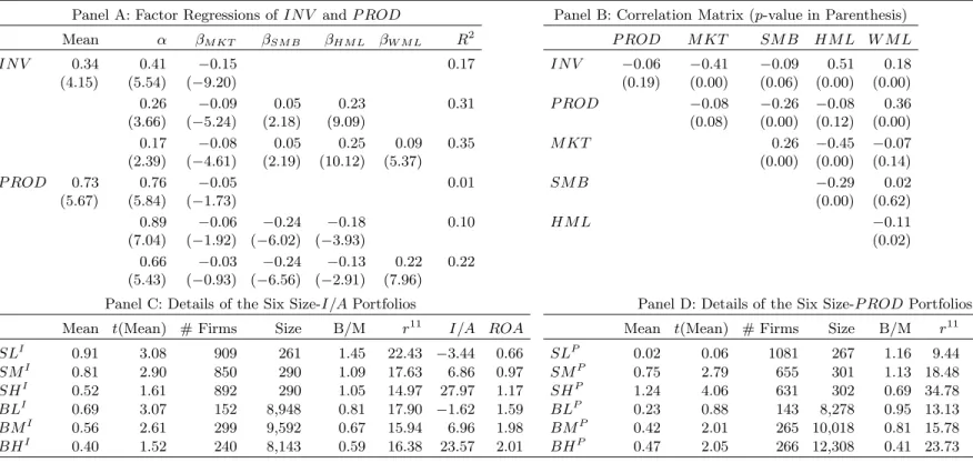
From Table 1, the averageIN V return in our sample is 0.34% per month (t= 4.15). Regressing IN V on M KT generates an alpha of 0.41% per month (t = 5.54) and a R2 of 17%. Regressing
IN V on the Fama and French (1993) model and the Carhart (1997) model reduces the alpha to 0.26% and 0.17% per month (t= 3.66 and 2.39), and increases theR2to 31% and 35%, respectively. (The data for the Fama-French factors and the momentum factor are from Kenneth French’s Web site.) Thus,IN V captures average return variations not subsumed by the other common factors.
IN V has a relatively high correlation of 0.51 withHM L (p-value = 0). This evidence is con-sistent with Xing (2006), who shows that an investment growth factor contains information similar to HM L and can explain the value effect roughly as well as HM L. Xing constructs her factor by sorting on the growth rate of capital expenditure. The average return of her factor is only 0.20% per month, albeit significant. We follow Lyandres, Sun, and Zhang (2007) in using a more comprehensive measure of investment that includes both long-term and short-term investments. As a result, our investment factor earns a higher average return.
Panel C of Table 1 provides more details on the six size-I/Aportfolios underlying theIN V fac-tor. Sorting onI/Agenerates a large spread inI/A: PortfolioSLI (small-size and low-investment) has an average I/Aof−3.44% per annum, whereas portfolioSHI (small-size and high-investment)
has an average of 28%. PortfolioSHI is also more profitable than portfolioSLI: The earnings-to-assets (ROA) of portfolioSHI is 1.17% per quarter versus 0.66% for portfolioSLI. Portfolio SLI also has a higher average prior 2–12 month return (from July of yeart−1 to May of yeart) than
port-folioSHI, 22% versus 15%. This evidence partially reflects the fact that low-investment firms have higher average future returns than high-investment firms. (We follow Fama and French (1993) in sorting stocks in June on accounting information at the last fiscal year-end to guard against the look-ahead bias.) The evidence does not mean that low-investment firms have higher average contem-poraneous returns. In untabulated results, we measure returns over the calendar yeart−1 and find
3.1.2 The Productivity Factor, P ROD
We constructP RODbased on earnings-to-assets, ROA. Using cash-flow-to-assets to measure pro-ductivity does not materially affect our results (not reported). We sort on current profitability, as opposed to expected profitability. The reason is that profitability is highly persistent (e.g., Fama and French 1995, 2000, 2006). In particular, Fama and French (2006) show that current profitabil-ity is the strongest predictor of future profitabilprofitabil-ity, meaning that current profitabilprofitabil-ity is highly correlated with the expected profitability, to which equation (3) applies.
BecauseP RODis most relevant for explaining momentum profits that are constructed monthly, we use a similar approach to construct P ROD. In particular, we use quarterly data to measure ROA. Indeed, using annual sorts on annual earnings-to-assets at the last fiscal year-end yields an insignificant average return of only five basis points per annum for the productivity factor. This evidence is consistent with that reported by Fama and French (2007, Table II).
However, we also find that the original earnings and momentum anomalies do not survive the frequency change from monthly to annual rebalancing either. Specifically, in June of each year t, we sort all NYSE, Amex, and NASDAQ stocks into ten deciles based on the NYSE breakpoints of the Standardized Unexpected Earnings (SU E) measured at the fiscal year-end of t−1, the average
SU E over the last fiscal year, the annual return over the calendar year t−1, and the 12-month
return from June of yeart−1 to May of year t. Monthly value-weighted returns of these portfolios
are calculated from July of yeartto June of yeart+1. Untabulated results show that none of these strategies generate mean excess returns or CAPM alphas that are significantly different from zero. Because theSU Eand momentum anomalies only exist in monthly rebalancing, it seems reasonable to construct the explanatoryP ROD factor in the same frequency.
Nevertheless, we emphasize that using quarterly earnings to construct P ROD, while using an-nual investment to constructIN V, is largely driven by data, not by theory. The growing literature on investment-based asset pricing does predict that earnings and prior returns can be related to time-varying expected returns.4 However, to the best of our knowledge, the theoretical literature has so far not addressed the question why earnings and momentum anomalies are more short-lived than others such as value and investment anomalies. This caveat also applies to our work.
4
See Berk, Green, and Naik (1999), Johnson (2002), and Sagi and Seasholes (2007) for recent examples that relate prior short-term returns to expected returns. Liu and Zhang (2007) document that recent winners have temporarily higher loadings than recent losers on the growth rate of industrial production. Liu, Whited, and Zhang (2007) show that an investment-based expected return model can partially explain the earnings anomaly.
To construct P ROD, each month from January 1972 to December 2006, we categorize NYSE, Amex, and NASDAQ stocks into three groups based on the NYSE breakpoints for the low 30%, middle 40%, and high 30% of the ranked values of quarterlyROA from at least four months ago. The choice of the four-month lag is conservative: Using shorter lags only serves to strengthen our re-sults (not reported). We use the four-month lag to ensure that the required accounting information is known before we form the portfolios. We also use the NYSE median market equity each month to split NYSE, Amex, and NASDAQ stocks into two groups. We form six portfolios from the intersec-tions of the two size and three ROAgroups. Monthly value-weighted returns on the six portfolios are calculated for the current month, and the portfolios are rebalanced monthly. TheP RODfactor is meant to mimic the common variations in returns related to firm-level productivity: P RODis the difference (high-minus-low productivity), each month, between the simple average of the returns on the two high-ROAportfolios and the simple average of the returns on the two low-ROAportfolios. From Panel A of Table 1, P ROD earns an average return of 0.73% per month (t = 5.67) from January 1972 to December 2006. Regressing theP RODreturn on the market factor, the Fama and French (1993) three factors, and the Carhart (1997) four factors yields large alphas of 0.76%, 0.89%, and 0.66% per month (t= 5.84, 7.04, and 5.43), andR2s of 1%, 10%, and 22%, respectively. This evidence means that, like IN V, P ROD also captures average return variations not subsumed by well-known common factors. Panel B reports thatP RODandW M Lhave a high correlation of 0.36 (p-value = 0). Intuitively, shocks to earnings are positively correlated with contemporaneous shocks to returns. Thus, we expect P ROD to have certain explanatory power for momentum profits.
Intriguingly, the correlation betweenIN V andP RODis only −0.06 (p-value = 0.19), meaning
no need to neutralize the two factors against each other. The low correlation is counterintuitive because one would expect that more profitable firms should invest more and that the two factors should be negatively correlated. The low correlation results from our use of quarterly earnings to constructP RODbut annual investment to constructIN V. If we instead use annual earnings data to construct the productivity factor, we find its correlation with IN V to be −0.20 (p-value = 0).
And if we use quarterly investment data to construct the investment factor, we find its correlation withP ROD to be −0.33 (p-value = 0). Thus, matching rebalancing frequency increases the
posi-tive correlation between investment and earnings, thereby increasing the magnitude of the negaposi-tive correlation between their factor mimicking portfolio returns.
Sort-ing onROAgenerates a large spread inROA: PortfolioSLP (small-size and low-productivity) has an averageROAof−1.78% per quarter, whereas portfolio SHP (small-size and high-productivity)
has an averageROAof 3.41%. The largeROAspread only corresponds to a modest spread in annual I/A: 11.4% versus 12.6%. The evidence helps explain the low correlation betweenIN V andP ROD reported earlier. And the ROA spread in small firms corresponds to a large spread in prior 2–12 month returns: 9.4% versus 34.8%, helping explain the high correlation betweenP RODandW M L. 3.2 Tests on Two-Way Sorted Portfolios
We report time series regressions of two-way sorted testing portfolios formed on size and momen-tum, size and book-to-market, and investment and profitability. We study momentum and value portfolios because these are arguably most important anomalies in the cross section. We also study investment and profitability portfolios because our factors are constructed on these characteristics.
3.2.1 Preliminaries
We start by describing the construction and the basic properties of testing portfolios.
3.2.1.1 The Size-Momentum Portfolios The 25 size-momentum portfolios are from Ken-neth French’s Web site. Fama and French (1996) use the “11/1/1” convention to measure momen-tum. For each montht, stocks are sorted on their prior returns from month t−2 tot−12 (skipping
montht−1), and the subsequent portfolio returns are calculated for the current montht. The 25 size
and 11/1/1-momentum portfolios are formed monthly as the intersection of five portfolios sorted on size and five portfolios sorted on prior 2–12 month returns. The monthly breakpoints are the NYSE market equity quintiles, and the monthly prior 2–12 month returns breakpoints are NYSE quintiles. Following Jegadeesh and Titman (1993), we also construct an alternative set of 25 size and mo-mentum portfolios using the “6/1/6” convention of momo-mentum. For each month t, we use NYSE breakpoints to sort stocks on their prior returns from month t−2 to t−7 (skipping month t−1),
and calculate the subsequent portfolio returns from month t to t+5. We also use NYSE market equity quintiles to sort all stocks independently each month into five size portfolios. The 25 size and 6/1/1-momentum portfolios are formed monthly as the intersection of the five size quintiles and the five quintiles based on prior 2–7 month returns.
Table 2 reports large momentum profits, especially in small firms. Panel A uses the “11/1/1” convention of momentum. The winner-minus-loser (W-L) average return varies from 0.64% per
month (t= 2.16) in the biggest-size quintile to 1.72% (t= 7.63) in the smallest-size quintile. In to-tal, 16 out of 25 size and momentum portfolios have significant CAPM alphas. The null hypothesis that the 25 CAPM alphas are jointly zero is strongly rejected by the GRS test: The test statis-tic (FGRS) is 6.22 (p-value = 0). More important, the CAPM alphas for the winner-minus-loser portfolios are significant positive across all five size quintiles. The small-stock W-L strategy, in particular, earns a CAPM alpha of 1.78% per month (t= 8.23). Consistent with Fama and French (1996), their three-factor model exacerbates the momentum anomaly: 18 out of 25 Fama-French alphas are significant. And the Fama-French alphas for theW-Lportfolios are all larger than their corresponding CAPM alphas. In particular, the small-stock W-L strategy earns a Fama-French alpha of 1.96% per month (t = 7.97). The reason is that losers have higher HM L-loadings than winners: Losers behave more like value stocks, and the Fama-French model predicts that losers should earn higher average returns, instead of lower average returns as we see in the data.
The results from the 25 size and 6/1/6-momentum portfolios are similar, but the magnitude of momentum profits is smaller than that with the 11/1/1-momentum. The mean excess return of the W-L portfolio ranges from 0.64% per month (t = 2.82) in the biggest-size quintile to 0.97% (t = 5.48) in the smallest-size quintile. The CAPM fails to explain the average returns of these testing portfolios: 13 out of 25 individual alphas are significant. And the GRS test rejects the model at the 1% level. In particular, the small-stockW-Lstrategy earns an alpha of 1.02% per month (t= 6.04). The Fama-French (1993) model again generates larger pricing errors than the CAPM. The W-L alpha from the Fama-French model ranges from 0.75% (t = 2.92) to 1.14% per month (t = 6.07).
3.2.1.2 The 25 Investment-Profitability Portfolios We sort all NYSE, Amex, and NAS-DAQ stocks into five profitability quintiles each month based on NYSE breakpoints of quarterly ROA from at least four months ago. Also, we sort all stocks independently in June of each year into five quintiles based on NYSE breakpoints of investment-to-assets at the last fiscal year-end. Taking intersections yields 25 investment and profitability portfolios. Their value-weighted returns are calculated for the current month, and the portfolios are rebalanced monthly.
Panel A of Table 3 reports descriptive statistics for the 25 investment-profitability portfolios. HighROAstocks earn higher average returns than low ROAstocks, especially among high invest-ment firms. And high investinvest-ment stocks earn lower average returns than low investinvest-ment stocks, especially among low ROA firms. The average high-minus-low ROA portfolio return varies from 0.40% per month (t= 1.64) in the lowest-I/Aquintile to 1.17% (t= 4.81) in the highest-I/A
quin-tile. The average low-minus-highI/Aportfolio return varies from an insignificant 0.16% per month in the highest-ROA quintile to 0.93% (t = 4.30) in the lowest-ROA quintile. The null hypothesis that all the CAPM alphas are jointly zero is rejected at the 1% level. Despite their higher average returns, highROAfirms have lowerSM Band HM Lloadings than lowROAfirms. Consequently, 12 out of 25 portfolios have significant alphas in the Fama-French (1993) model, in contrast to only five significant alphas out of 25 in the CAPM.
3.2.1.3 The 25 Size-B/M Portfolios We obtain the 25 Size-B/M portfolios from Kenneth French’s Web site. These portfolios are the intersections of five size portfolios and five B/M portfo-lios at the end of each June. The size breakpoints for yeartare the NYSE market equity quintiles at the end of June oft. B/M for year tis the book equity for the last fiscal year-end in t−1 divided
by market equity for December of t−1. The B/M breakpoints are also NYSE quintiles.
Confirming many previous studies, Panel B of Table 3 shows that value stocks earn higher average returns than growth stocks. The average high-minus-low (H-L) return is 1.09% per month (t = 5.08) in the smallest-size quintile versus 0.25% (t = 1.20) in the biggest-size quintile. The CAPM cannot explain the value premium: 15 out of 25 portfolios have significant alphas and the GRS statistic is 4.25 (p-value = 0). Further, three out of fiveH-Lstrategies have significant alphas. In particular, the small-stock H-L portfolio earns a positive alpha of 1.32% per month (t= 7.10). The Fama and French (1993) model represents an impressive improvement over the CAPM in capturing the average returns across the 25 size-B/M portfolios. The number of significant alphas reduces from 15 to only six. The small-stock H-L alpha is reduced to 0.68% per month (albeit still significant, t = 5.50), which is 48% lower than its CAPM alpha. The reason is that, as highlighted in Fama and French (1996), their three-factor model generates systematic variations in factor loadings: Small stocks have higher SM B loadings than big stocks, and value stocks have higherHM Lloadings than growth stocks. The averageR2 across the 25 portfolios is 89%, so even small intercepts are often distinguishable from zero.
3.2.2 Neoclassical Regressions: The Size-Momentum Portfolios
The neoclassical model outperforms traditional models in pricing the size-momentum portfolios.
3.2.2.1 Benchmark Estimation Table 4 reports the neoclassical regressions of the size and momentum portfolios. Panel A shows that the W-L 11/1/1-momentum strategy has a significant
alpha of 0.89% per month (t= 3.25) in the smallest size quintile and 0.61% (t= 2.36) in the second size quintile. But the alphas are insignificant in the three other size quintiles. In contrast, the W-L alpha is significant across all five size quintiles in both the CAPM and the Fama and French (1993) model (see Table 2). This performance improvement is noteworthy. For example, although still significant (t= 3.25), the small-stockW-Lalpha of 0.89% per month in the neoclassical model represents a reduction of 50% in magnitude from its CAPM alpha (1.78%) and a reduction of 55% from its Fama-French alpha (1.96%). Further, the average magnitude of the W-L alphas in the neoclassical model is 0.37% per month. In contrast, the magnitude is 1.21% in the CAPM and 1.38% per month in the Fama-French model. Finally, eight out of the 25 individual alphas are significant, giving rise to an overall rejection of the neoclassical model by the GRS test at the 1% level. However, the number of significant alphas in the neoclassical model (8) is much lower than that in the CAPM (16) and that in the Fama-French model (18).
The results using the 6/1/6-momentum portfolios are largely similar. Although the neoclassical model is rejected using the 25 portfolios, the number of significant alphas (7) is lower than that in the CAPM (13) and that in the Fama-French (1993) model (13). More important, none of the fiveW-L alphas in our model are significant. In particular, the small-stockW-Lalpha is 0.34% per month (t = 1.53). This neoclassical alpha represents a reduction in magnitude of 67% from the CAPM alpha (1.02% per month,t= 6.04) and a reduction of 70% from the Fama-French alpha (1.14%,t= 6.07).
3.2.2.2 Sources of Explanatory Power for the Neoclassical Model The relative suc-cess of the neoclassical model in explaining momentum profits derives from two sources. First, the P ROD-loadings of momentum portfolios go in the right direction in explaining their average returns. Table 4 shows that winners have higher P ROD-loadings than losers across all five size groups. The magnitude of the loading spreads, significant in all cases, ranges from 0.64 to 0.88 in Panel A for the 11/1/1-momentum and from 0.45 to 0.61 in Panel B for the 6/1/6-momentum. This evidence suggests that, not surprisingly, winners are more profitable than losers.
Second, remarkably, the IN V-loadings also go in the right direction in explaining momentum profits: Winners have higher IN V-loadings than losers. The magnitude of the loading spreads, again significant across all size groups, ranges from 0.68 to 0.96 for the 11/1/1-momentum and from 0.47 to 0.71 for the 11/1/1-momentum. The IN V-loading pattern is counterintuitive: We would expect that winners with high valuation ratios should invest more and have lower loadings on the low-minus-high IN V factor than losers with low valuation ratios.
To understand the driving forces behind these loading patterns, we follow the event-study ap-proach of Fama and French (1995) to examine howROAandI/Avary across the testing portfolios. To preview the results: Winners indeed have higher contemporaneous investment-to-assets than losers at the portfolio formation month. But more important, winners also have lower investment-to-assets than losers starting from two to four quarters prior to the portfolio formation. Because IN V is rebalanced annually, the higher IN V-loadings for winners accurately reflect their lower investment-to-assets several quarters prior to the portfolio formation.
Specifically, for each portfolio formation month t = January 1972 to December 2006, we cal-culate quarterly ROAs and annual I/As for t+m, m=−60, . . . ,60. TheROA and I/A for t+m
are then averaged across portfolio formation months t. ROA is the most recent ROA relative to portfolio formation month t. Figure 1 reports the details for the 25 size and 11/1/1-momentum portfolios. The results for the 25 size and 6/1/6-momentum portfolios are similar (not reported). For a given portfolio, we plot the median ROAs andI/As among the firms in the portfolio.
From Panel A of Figure 1, although winners have higherI/As at the portfolio formation month t, winners have lower I/As than losers from month t−60 to month t−8. Consistent with this
event-time evidence, Panel B shows that winners have higher contemporaneous I/As than losers in the calendar time in the smallest-size quintile. We define the contemporaneous I/Aas the I/A at the current fiscal year-end. For example, if the current month is March or September 2003, the contemporaneous I/A is the I/A at the fiscal year-end of 2003. More important, Panel C shows further that winners also have lower lagged or sorting-effective I/As than losers in the smallest-size quintile. We define the sorting-effective I/A as the I/A on which an annual sort on I/A in each June (as in our construction ofIN V) is based. For example, if the current month is March 2003, the sorting-effective I/Ais the I/Aat the fiscal year-end of 2001 because the annual sort onI/A is in June 2002. If the current month is September 2003, the sorting-effectiveI/Ais theI/Aat the fiscal year-end of 2002 because the applicable sort on I/A is in June 2003. Because IN V is rebalanced annually, the lower sorting-effectiveI/As of winners explain their higherIN V-loadings than losers. As expected, Figure 1 also shows that winners have higher ROAs than losers for about five quarters before and 20 quarters after the portfolio formation month (Panel D). In the calendar time, winners have consistently higher ROAs than losers, especially in smallest-size quintile (Panels E and F). This evidence explains the higherP ROD-loadings for the winners documented in Table 4.
3.2.2.3 Quarterly Investment Factor To verify that the annual rebalancing ofIN V is in-deed the driving force of the IN V-loading pattern across momentum portfolios, we experiment with an alternative investment factor, denoted IN VQ, constructed on quarterly investment data. To preview the results, the loading pattern is reversed once we replaceIN V withIN VQ.
We measure quarterly investment-to-assets as the change in gross property, plant, and equip-ment (Compustat quarterly item 42) plus the change in inventory (item 38) divided by lagged total assets (item 44). This definition is the exact quarterly counterpart of our definition based on annual data (see Appendix B). Each month from January 1975 to December 2006, we categorize NYSE, Amex, and NASDAQ stocks into three groups based on the NYSE breakpoints for the low 30%, middle 40%, and high 30% of the ranked values of quarterly I/A from at least four months ago. (The starting point of the sample is restricted by the availability of quarterly investment data.) We also use the NYSE median market equity each month to split all stocks into two size groups. We form six portfolios from the intersections of the two size and threeI/Aportfolios and calculate monthly value-weighted returns on the six portfolios for the current month. IN VQis the difference (low-minus-high investment), each month, between the simple average of the returns on the two low-I/A portfolios and the simple average of the returns on the two high-I/A portfolios.
The IN VQ factor earns an average return of 0.49% per month (t = 3.56). Table 5 reports neoclassical factor regressions withIN V replaced by IN VQ. Most important, the W-L portfolios now have negative, albeit mostly insignificant, loadings on IN VQ. This finding contrasts with the evidence in Table 4 that the W-L portfolios have significant positive loadings on the annual investment factor, IN V. The P ROD-loadings are similar across the two tables. As a result of the negativeIN VQ-loadings of theW-Lportfolios, the magnitude of the alphas in Table 5 is in general higher than that in Table 4. In particular, the small-stock W-L 11/1/1-momentum portfolio has an alpha of 1.28% per month (t = 3.83), which is about 30% higher than the alpha of 0.89% in Table 4. And the small-stockW-L6/1/6-momentum portfolio has an alpha of 0.65% per month (t = 2.54), which is about 48% higher than the alpha of 0.34% in Table 4.
3.2.2.4 Alternative Neoclassical Factor Specifications To evaluate the relative role of the neoclassical factors in driving momentum profits, we explore two alternative two-factor specifica-tions: M KT+IN V andM KT+P ROD. BothIN V andP RODhelp reduce the overall magnitude of the alphas, butP ROD seems more important. For example, Panel A of Table 6 shows that four out of fiveW-L11/1/1-momentum alphas are significant and the average magnitude of these alphas
is 0.96% per month in the two-factor model withM KT andIN V. In contrast, only two out of five W-L alphas are significant in the two-factor model with M KT and P ROD, although the average magnitude of these alphas is 0.67% per month. Thus, adding IN V further reduces the average magnitude of theW-Lalphas from 0.67% to 0.37% per month in the benchmark neoclassical model. From Panel B, using the 6/1/6-momentum portfolios yields largely similar results.
3.2.3 Neoclassical Regressions: The Investment-Profitability Portfolios
The neoclassical model outperforms traditional factor models in explaining the average returns across the 25 investment-profitability portfolios.
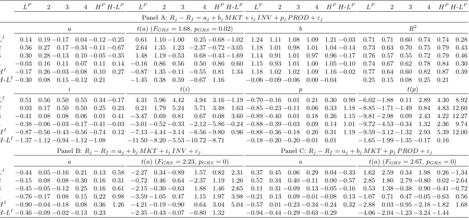
Panel A of Table 7 reports the neoclassical three-factor regressions. Although the model is rejected overall with a GRS statistic of 1.68 (p-value = 0.02), only two out of 25 alphas are individ-ually significant. The number of significant alphas is low relative to that in the CAPM (five) and to that in the Fama-French (1993) model (12). Further, only one out of five high-minus-lowROA portfolios (H-LP) has a significant alpha: The alpha is actually negative,
−0.67% per moth (t = −3.05), so our model appears to overfit. In contrast, three out of fiveH-LP alphas are significant
in the CAPM, and all five of them are significant in the Fama-French model. More important, the average magnitude of theH-LP alphas is also lower in our model: 0.34% per month versus 0.71% in the CAPM and 0.98% in the Fama-French model. Our model also does a good job in describing the five high-minus-lowI/Aportfolio (H-LI) returns. From Panel A, none of the five H-LI alphas are significant, whereas three out of five are significant in the CAPM and in the Fama-French model. More important, the average magnitude of theH-LI alphas is also lower in our model: 0.17% per month versus 0.55% in the CAPM and 0.39% in the Fama-French model.
As expected, high ROA firms have significantly higher P ROD-loadings than low ROA firms, and low-investment firms have significantly higher IN V-loadings than high-investment firms. The systematic variations in the neoclassical factor loadings across the investment-profitability portfolios (in the same direction as their average returns variation) explain the better empirical performance of our model relative to the CAPM and the Fama-French (1993) model.
In the benchmark specification (Panel A of Table 7), theIN V-loadings do not differ significantly across extreme ROAportfolios, and theP ROD-loadings do not differ significantly across extreme investment portfolios. The evidence is consistent with the low correlation betweenIN V andP ROD (−0.06, see Table 1). Consequently, droppingP RODfrom the factor specification makes the
investment alphas (Panel B). And dropping IN V makes the high-minus-low investment alphas significantly negative, but does not materially affect the high-minus-low ROAalphas (Panel C).
3.2.4 Neoclassical Regressions: The Size-B/M Portfolios
The neoclassical model outperforms the CAPM but underperforms the Fama-French (1993) model in explaining the average returns of the 25 size-B/M portfolios. But our model does exceptionally well in explaining the low average return of the small-growth portfolio that consists of firms in the smallest-size quintile and lowest-B/M quintile.
Panel A of Table 8 shows that, while the Fama-French (1993) model produces six significant alphas out of 25 size-B/M portfolios, the neoclassical model produces 11. Further, three out of five H-Lalphas are significant in our model versus only two out of five in the Fama-French model. The average magnitude of theH-Lalphas is also higher in our model: 0.45% versus 0.30% per month. And the average R2 is lower in our model: 73% versus 91%. But the average magnitude of the 25 alphas is 0.27% per month, which is identical to that from the Fama-French model.
More intriguingly, the small-growth portfolio earns a CAPM alpha of −0.63% per month (t= −2.61), a Fama-French alpha of−0.52% (t=−4.48), but only a tiny neoclassical alpha of −0.03%
(t =−0.10). This evidence is impressive because the small-growth anomaly is notoriously difficult
to explain for consumption-based asset pricing. For example, Campbell and Vuolteenaho (2004, Table 4) show that the small-growth portfolio is particularly risky in their two-beta model with both cash-flow and discount-rate betas exceeding those of the small-value portfolio. As a result, their two-beta model fails to explain the small-growth anomaly. And the literature has attributed the abnormally low return for small-growth firms to short-sale constraints and other limits to arbitrage (e.g., Lamont and Thaler 2003, Mitchell, Pulvino, and Stafford 2002).
The neoclassical model clearly dominates the CAPM in explaining the average 25 size-B/M portfolio returns. In total, 15 out of the 25 CAPM alphas are significant. The small-stockH-Lalpha in the CAPM is 1.32% per month (t= 7.10). Our model reduces this alpha by about 40% to 0.78% per month, albeit still significant (t= 3.67). The average magnitude of theH-Lalphas is 0.81% per month in the CAPM, and our model reduces this magnitude by about 45% to 0.45% per month.
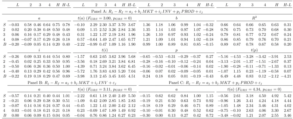
The IN V- andP ROD-loadings shed light on the explanatory power of the neoclassical model for the 25 size-B/M portfolios. From Panel A of Table 8, value stocks have higher IN V-loadings than growth stocks. The loading spreads, ranging from 0.69 to 1.00, are all at least 4.5 standard
errors from zero. TheP ROD-loading pattern is more complicated. TheH-Lspread in theP ROD -loading is close to zero across the three middle size quintiles. In the smallest-size quintile, theH-L portfolio has a significant positive P ROD-loading of 0.27 (t = 2.53) because the small-growth portfolio has a large negative P ROD-loading of −0.65 (t = −5.16). However, in the biggest-size
quintile, theH-Lportfolio has a large negative P ROD-loading of−0.43 (t=−4.21). In particular,
the big-growth portfolio has a positiveP ROD-loading of 0.24 (t= 6.49).
The two-factor neoclassical specifications in Panels B and C in Table 8 further illustrate the relative roles of P ROD and IN V. The alpha of the small-growth portfolio is −0.57% per month
(t = −2.22) in the two-factor M KT +IN V model, meaning that IN V does not help explain
the portfolio’s low average returns. But the alpha is only −0.15% (t = −0.56) in the two-factor
M KT +P RODmodel, meaning thatP ROD helps a lot. However, IN V helps reduce the overall magnitude of the alphas for other portfolios in the 25 size-B/M universe. The average magnitude of the H-L alphas across the size quintiles is 0.44% per month in theM KT +IN V model (close to that in the benchmark specification), but is 0.86% in theM KT +P RODmodel.
Somewhat surprisingly, the small-growth portfolio has a lower P ROD-loading than the small-value portfolio. The evidence seems inconsistent with Fama and French (1995), who document that growth firms are more profitable than value firms in the 1963–1992 sample. In untabulated results, we apply their empirical methods to our 1972–2006 sample. We find that growth firms have persistently higher ROAs than value firms in the biggest-size quintile for 11 years surrounding the portfolio formation year. But in the smallest-size quintile, growth firms have higher ROAs than value firms before, but have lower ROAs after the portfolio formation. In the calendar time, a striking downward spike ofROAappears for the small-growth portfolio over the past decade. The ROAstarts at about 0.50% per quarter in 1997, drops rapidly to about−7% in 2003, before rising
back to 0.50% in 2004. (See also related evidence in Fama and French 2001, 2004.) The dramatic ROAdeterioration of the small-growth firms over the past decade gives rise to their abnormally low P ROD-loadings. We also verify that the small-stock H-Lportfolio has a negativeP ROD-loading in the 1972–1995 sample before the downward spike occurs.
3.3 Tests on One-Way Sorted Portfolios
In this subsection, we test the neoclassical factor model using deciles formed on financial distress, earnings surprises, accruals, net issues, price, and asset growth. We use earnings-to-price portfolios as a representative of the array of one-way sorted value and growth portfolios
studied by, for example, Fama and French (1996). All the other anomaly variables have recently received much attention in the empirical finance and accounting literature.
3.3.1 The Distress Deciles
The neoclassical model is successful in explaining the financial distress anomaly. We form ten deciles on Campbell, Hilscher, and Szilagyi’s (2007) distress measure. We largely follow their pro-cedure in constructing the measure (see Appendix B).5 Each month from June 1975 to December 2006, we sort all NYSE, Amex, and NASDAQ stocks into ten deciles using the NYSE breakpoints of distress from at least four months ago. (The starting point of the sample is restricted by the availability of the data items required to construct the distress measure.) Monthly value-weighted portfolio returns are calculated for the current month.
Panel A of Table 9 reports that, consistent with Campbell, Hilscher, and Szilagyi (2007), more distressed firms earn lower average returns than less distressed firms. The high-minus-low (H-L) distress portfolio has an average return of−0.89% per month (t=−3.04). Controlling for traditional
risk measures only makes matters worse: More distressed firms are riskier than less distressed firms according to traditional factor models. The market beta of theH-Lportfolio is significantly positive, 0.53 (t= 5.79), meaning that its CAPM alpha of−1.23% per month (t=−4.15) has an even higher
magnitude than its average return. In total, five out of ten alphas are significant, leading to an overall rejection of the model (p-value = 0). The results from the Fama-French (1993) model are largely similar. The H-L portfolio has a SM B-loading of 0.65 (t = 5.24) and a market beta of 0.43 (t = 5.09). The Fama-French alpha is−1.34% per month (t=−5.22). Further, six out of ten
deciles have significant alphas, and the GRS test rejects the model (FGRS = 3.76,p-value = 0). More important, the neoclassical model generates an insignificant alpha of 0.18% per month (t = 0.83) for theH-L portfolio. Although two out of ten deciles have significant neoclassical alphas, the model cannot be rejected using the GRS test (FGRS = 1.68 andp-value = 0.08). TheP ROD -loading goes in the right direction in explaining the distress anomaly. More distressed firms have lower P ROD-loadings than less distressed firms: The loading spread is −1.48 (t =−14.59). This
evidence makes sense because the distress measure has a strong negative relation with profitability (see equation B.1), meaning that more distressed firms are less profitable than less distressed firms. In untabulated results, we directly calculate time series averages of portfolio ROAfor the ten
5
We have used portfolios formed on Ohlson’s (1980)O-Score and obtained similar results. We also have used Alt-man’s (1968)Z-score, but the CAPM explains well the averageZ-score portfolio returns in our sample (not reported).
distress deciles. We measure portfolio ROA as the value-weighted average ROAs across all the stocks in a given portfolio, in which the weights are given by the market equity to be consistent with the calculations of portfolio returns. The portfolio averageROAdecreases monotonically from 3.43% per quarter for the lowest-distress decile, to 1.74% for the fifth decile, and further to−2.15%
per quarter for the highest-distress decile. The averageROAspread of 5.58% per quarter between the two extremes is more than 25 standard errors from zero.
From Panel A of Table 9, the highest-distress decile also has a lower IN V-loading than the lowest-distress decile: The loading spread is −0.53 (t =−3.10). In untabulated results, we
calcu-late time series averages of portfolioI/A for the distress deciles. We measure portfolio I/Aas the value-weighted averageI/As across all the stocks in a given portfolio, in which the weights are given by the market equity. We find that the average I/Ais 11.83% per annum in the highest-decile and 8.88% in the lowest-distress decile. TheI/A-spread of 2.95% per annum is significant (t = 2.55). Thus, theIN V-loading is consistent with the underlying investment pattern. One possible reason for the investment pattern is that the distress measure has a positive loading on the market-to-book (see equation B.1), meaning that more distressed firms can be high-investing growth firms.
3.3.2 The Earnings Surprises Deciles
The neoclassical factor model outperforms traditional factor models in explaining the earnings anomaly, the “granddaddy” of underreaction events in the language of Fama (1998, p. 286). To construct the testing portfolios, we rank all NYSE, Amex, and NASDAQ stocks each month based on the NYSE breakpoints of their most recent past SU E. Monthly value-weighted returns on the SU E portfolios are calculated for the current month, and the portfolios are rebalanced monthly.
From Panel B of Table 9, sorting on SU E produces an average-return spread of 1.17% per month (t = 8.05) between the two extreme deciles. The CAPM alpha of the H-L SU E portfolio is 1.22% per month (t= 8.50). Eight out of ten portfolios have significant alphas, and the CAPM is strongly rejected by the GRS test. The Fama-French (1993) model cannot explain the earnings anomaly either: Eight out of ten alphas are significant and the model is also rejected by the GRS test (FGRS = 9.64, p-value = 0). And the H-L SU E portfolio alpha remains at 1.22% per month (t = 8.00). The neoclassical model reduces the alpha from 1.22% per month to 0.89%, which rep-resents a reduction of 27%. But the alpha remains significant (t= 6.24). The overall performance of the model is also improved: The number of significant alphas across the deciles is reduced to four, although the model is still rejected by the GRS test (FGRS = 4.57,p-value = 0).
Our model improves on the traditional factor models because the H-L SU E portfolio has a positiveP RODloading of 0.33 (t= 5.07). In untabulated results, we find that the average portfolio ROAincreases from 1.12% per quarter for the lowest-SU E decile to 1.68% for the fifthSU E decile and further to 2.60% for the highest-SU Edecile. The averageROAspread between the two extreme deciles is only 1.48% per quarter, albeit significant (t = 12.16). This low magnitude of theROA spread helps explain why our model is only partially successful in explaining the earnings anomaly.
3.3.3 The Accrual Deciles
In June of each yeart, we sort all NYSE, Amex, and NASDAQ stocks into ten deciles based on the NYSE breakpoints of accruals at the last fiscal year-end of t−1. Monthly value-weighted portfolio
returns are calculated from July of year t to June of year t+1. Panel A of Table 10 shows that, consistent with Sloan (1996), high accrual firms earn lower average returns than low accrual firms and the average H-L accrual portfolio earns an average return of−0.52% per month (t=−4.13).
The CAPM and the Fama-French (1993) model cannot explain the accrual anomaly: The average H-L accrual portfolio earns a CAPM alpha of−0.55% per month (t=−4.41) and a Fama-French
alpha of−0.57% (t=−4.35). The zero-cost portfolio has traditional factor loadings all close to zero.
In the neoclassical model, theH-Laccrual portfolio has near zero loadings onM KT andP ROD but a negative IN V-loading of −0.51 (t = −5.33). As a result, the zero-cost portfolio earns an
alpha of−0.38% per month (t =−2.97) in our model, which represents a reduction in magnitude
of about 33% from its Fama-French alpha. The GRS test still rejects our model, however. In untabulated results, we find that the average portfolio I/A increases monotonically from 4.86% per annum for the lowest-accrual decile to 9.47% for the fifth decile and further to 20.06% for the highest-accrual decile. The significantI/A-spread of 15.21% per annum between the two extremes (t = 6.61) explains theIN V-loading pattern across the accrual deciles.
3.3.4 The Net Stock Issues Deciles
In June of each yeart, we sort all NYSE, Amex, and NASDAQ stocks into ten deciles based on the NYSE breakpoints of net stock issues at the last fiscal year-end. Monthly value-weighted portfolio returns are calculated from July of year t to June of year t+1. From Panel B of Table 10, firms with high net issues earn lower average returns than firms with low net issues: TheH-Lnet issues portfolio earns an average return of −0.96% per month (t = −5.23). The CAPM cannot explain