Detecting structural
differences in tail dependence
of financial time series
by Carsten Bormann and Melanie Schienle
No. 122 | JANUARY 2019
Impressum
Karlsruher Institut für Technologie (KIT) Fakultät für Wirtschaftswissenschaften Institut für Volkswirtschaftslehre (ECON)
Kaiserstraße 12 76131 Karlsruhe
KIT – Die Forschungsuniversität in der Helmholtz-Gemeinschaft Working Paper Series in Economics
No. 122, January 2019 ISSN 2190-9806
Detecting Structural Differences in Tail
Dependence of Financial Time Series
Carsten Bormann
Karlsruhe Institute of Technology
and
Melanie Schienle
Karlsruhe Institute of Technology
ABSTRACT
An accurate assessment of tail inequalities and tail asymmetries of financial returns is key for risk management and portfolio allocation. We propose a new test procedure for detecting the full extent of such structural differences in the dependence of bivariate extreme returns. We decompose the testing problem into piecewise multiple comparisons of Cramér-von Mises distances of tail cop-ulas. In this way, tail regions that cause differences in extreme dependence can be located and consequently be targeted by financial strategies. We derive the asymptotic properties of the test and provide a bootstrap approximation for finite samples. Moreover, we account for the multiplicity of the piecewise tail copula comparisons by adjusting individual p-values according to multiple testing techniques. Monte Carlo simulations demonstrate the test’s superior finite-sample properties for common financial tail risk models, both in the i.i.d. and the sequentially dependent case. During the last 90years in US stock mar-kets, our test detects up to 20% more tail asymmetries than competing tests. This can be attributed to the presence of non-standard tail dependence struc-tures. We also find evidence for diminishing tail asymmetries during every major financial crisis – except for the 2007-09 crisis – reflecting a risk-return trade-off for extreme returns.
Keywords: Tail dependence, tail copulas, tail asymmetry, tail inequality, ex-treme values, multiple testing
1
INTRODUCTION
Asymmetric dependence both within and between bivariate extreme returns in different market conditions is not only a key criterion for asset and risk man-agement, but also a main focus of market supervision. During financial crises, financial markets exhibit pronounced cross-sectional co-movements of (lower) tails of return distributions. Thus, the tendency of joint extreme events inten-sifies, see e.g. Longin and Solnik (2001); Ang and Chen (2002); Li (2013). For investment strategies, this should be taken into account by timely and adequate re-allocations of assets, e.g. profiting from arbitrage trading opportunities, and by appropriate adjustments of hedging decisions. Conversely, risk managers and market supervisors might need to set larger capital buffer requirements if the tendency for joint occurrences of extreme losses rises in times of market dis-tress. Specifically aiming at dependence between extreme events, we provide a robust non-parametric statistical test against tail dependence differences. The test accurately detects all types and the full extent of deviations between two tail dependence functions. Our test procedure is based on multivariate ex-treme value techniques which remain valid during turbulent market periods, e.g. Mikosch (2006). Particular to finance, Ang and Chen (2002), Patton (2006), Chollete et al. (2011), Li (2013) document the economic merits for asset diversi-fication of asymmetric dependence structures, e.g. for optimal portfolio alloca-tion. Under adverse market conditions, standard linear dependence measures are flawed which demands for alternative statistical models. Most prominently, the Gaussian copula is a convenient tool to model dependence near the mean of multivariate distributions. However, it is not capable of measuring dependence in the far tails (Embrechts (2009)). Furthermore, our test connects concepts of multivariate extreme value theory with multiple testing techniques. Recently, the latter have gained in practical importance in times of abundant data and the risk of data snooping, see e.g. in the finance context Barras et al. (2010), Bajgrowicz and Scaillet (2012) and Bajgrowicz et al. (2015) .
differ-ences in tail dependence structures which we measure with tail copulas de-noted by Λ(x(1), x(2)),(x(1), x(2))∈
R2+. A tail copula is a functional of the complete
tail dependence. The flexibility of using empirical tail copulas avoids possi-ble parametric misspecification risk; see e.g. Longin and Solnik (2001); Patton (2013); Jondeau (2016) for parametric approaches. Furthermore, the general-ity of this approach is in sharp contrast to established approaches, which only estimate and compare scalar summary measures of extreme dependence, such as the tail dependence coefficient (Hartmann et al. (2004), Straetmans et al. (2008)), or the tail index of aggregated tails (Ledford and Tawn (1996)). Specif-ically, we compare tail copulas over their entire relevant domain in a locally piecewise way. Thus, we study a multiple testing problem of tail copula equal-ity. Piecewise testing allows to pin down specific quantile regions where tail dependence differences are most serious. Such areas then indicate those types of extreme market conditions that typically cause tail asymmetry (inequality). Moreover, our test is still consistent if one (or both) of the two considered tail copulas is non-exchangeable, i.e. Λ(x(1), x(2))6= Λ(x(2), x(1)). Existing procedures
fail to address such intra-tail asymmetric dependence structures. Therefore, for non-exchangeable tail copulas, those tests are inconsistent.
Our test builds on the idea of a two-sample goodness-of-fit test for tail copu-las as in Bücher and Dette (2013). However, for increased sensitivity against vi-olations of the null, we compare both tail copulas in a piecewise way on disjoint subintervals of the unit simplex hull. This way, a number of individual tests against tail dependence equality is carried out. For an accurate overall assess-ment, we use multiple testing principles, such as the familywise error control and the false discovery rate, to jointly control the error rate of all marginal tests. Asymptotic properties of the test are provided. Moreover, a multiplier bootstrap procedure is suggested by extending ideas of Bücher and Dette (2013) to non-i.i.d. data.
A simulation study with widely used factor and Clayton copulas reveals the test’s attractive finite sample properties both for i.i.d. and sequentially
de-pendent time series data. In standard cases, our test is slightly superior to competing tests, while it is much more powerful in case of intra-tail asymmet-ric copulas. Simulation results strongly suggest that accounting for time series dynamics is essential. This can be achieved by either GARCH pre-filtering or by directly adjusting the bootstrap approximation for serial dependence.
In an empirical application, we establish tail asymmetry dynamics of 49 US stock sectors for the last 90 years, i.e. dynamics of the differences between upper and lower tails of all bivariate industry pairs. We find empirical evidence that tail asymmetries substantially diminish in times of financial distress. The only strong exception is the 2007-2009 financial crisis which apparently was completely different in structure than any other crisis. We conclude dependence between extreme gains increases in crisis. As the danger of joint extreme losses surges during bear markets, this finding documents a type of extreme risk-return trade-off as joint extreme gains are more likely compensating for the increased risk of joint extreme losses. This contrasts with other studies that analyze and compare market index pairs. Overall, our test detects up to 20%
more tail asymmetries than competing tests. This can specifically be attributed to tail events not detected by standard tail dependence measures as the tail dependence coefficient (TDC) (Hartmann et al. (2004); Jondeau (2016)), or the tail copula-based test by Bücher and Dette (2013). Thus, our test could serve as a more accurate tool for investors when assessing tail asymmetry in the market, e.g. our test reveals more opportunities for improved tail asymmetry-based portfolio allocation strategies. In the Appendix D of the online supplement material, we also study tail inequalities between foreign exchange rates.
This paper is structured as follows. Section 2 introduces theoretical results on tail dependence necessary for the testing procedures. Section 3 introduces our testing technique. It also provides asymptotic properties and respective fi-nite sample versions of the test procedures. Section 4 studies the fifi-nite sample performance in a thorough simulation study, and Section 5 studies tail asym-metries of US stock sectors. Additionaly, we analyze tail inequalities between
major foreign exchange rates in Appendix D of the online material. Finally, Section 6 concludes. All proofs are contained in the Appendix of the paper.
2
TAIL DEPENDENCE AND TAIL COPULAS
To understand the test idea and test statistics, we shortly introduce necessary tools from extreme value statistics. A complete treatment thereof can be found e.g. in de Haan and Ferreira (2006). For a two-dimensional (random) return vector X= (X(1), X(2)) its marginal components X(i) are assumed to have a
con-tinuous distribution function Fi(x(i)) and thus a well-defined marginal quantile
function Fi−1 fori= 1,2.
Our test is based on the full dependence structure in the tails captured by a tail copula. Note, standard dependence measures such as point corre-lations, quantify the likelihood of aligned return movements of X(1) and X(2).
However, if returns of both assets are extreme, i.e. {X(i) > F−1
i (1 − t)}, or
{X(i) < Fi−1(t)}, i = 1,2, for t → 0, standard dependence measures are insuf-ficient, and thus measures that focus on the tails should be used, see e.g. Embrechts (2009). For example, the Gaussian copula, which is completely parametrized by the correlation coefficient, is unable to model any tail depen-dence. That is to say, dependence may vary over different parts of the distribu-tion, and correlation may be unable to measure dependence in the tails.
Measuring the complete tail dependence between X(1) and X(2), the upper
and lower tail copula ΛUX(x(1), x(2)),ΛLX(x(1), x(2)),x:= (x(1), x(2)),x∈R2
+, are defined by ΛUX(x(1), x(2)) := lim t→0t −1 P(X(1) > F1−1(1−tx (1) ), X(2) > F2−1(1−tx(2))), ΛLX(x(1), x(2)) := lim t→0t −1 P(X(1) < F1−1(tx (1)), X(2) < F−1 2 (tx (2))), t∈ R+ (1)
i.e. the tail copula measures how likely both components jointly exceed ex-treme quantiles, see e.g. de Haan and Ferreira (2006), Schmidt and Stadtmüller
(2006), for details. If ΛUX(x)>0 (ΛLX(x) >0), gains (losses) of X are said to be tail dependent. For the sake of notational brevity, we omit the superscripts U and
L unless it becomes important. With x= (1,1), the tail copula boils down to the tail dependence coefficient (TDC), ι := Λ(1,1). The TDC is a standard tool in fi-nancial applications to measure tail dependence, e.g. Frahm et al. (2005), Aloui, Aïssa and Nguyen (2011), Garcia and Tsafack (2011). However, the TDC covers only a fragment of tail dependence, namely dependence between joint quantile exceedances of marginals thresholds along the line(F1−1(1−t), F2−1(1−t)), t →0. In contrast, the tail copula varies marginal thresholds as (x(1), x(2)) ∈
R2+, and
describes tail association for every possible tail event. It can be shown that
ΛX(x(1), x(2)) ∈ [0,min(x(1), x(2))], and Λ
X(ax) = aΛX(x), a ∈ R. Due to this
homo-geneity of the tail copula, it is sufficient to analyze the tail copulaΛX(x) only on the domain S ⊂R2, where we set wlog S :={(x(1), x(2)) :x(1), x(2) ≥0, ||x||
1 = 1}, as
the unit simplex hull. This restriction to the relevant domain of the tail copula reduces computational efforts in practical implementation and is key for our test.
In the following, we require the tail copulas of interest to exist and work in the following setup.
Assumptions 1. For a bivariate random vectorX, we assume that
(A1) X1, . . . ,Xnare i.i.d. observations of X∼FX.
(A2) FX is in the max-domain of a bivariate extreme value distribution with tail copula ΛX>0.
Assumption (A1) is standard in extreme value theory, yet restrictive for fi-nancial time series. We use it to illustrate our test idea and to formally derive its statistical properties. In Section 4.1, we then show how (A1) can be re-laxed to stationarity and strongly mixing making the test applicable to financial data. Assumption (A2) requires that sample tails can be modeled by bivariate extreme value distributions and are asymptotically dependent for nonparamet-ric estimators to be unbiased, see Schmidt and Stadtmüller (2006) for details
why this excludes ΛX(x) = 0. Standard distributions with actual tail depen-dence, such as e.g. the bivariatet-distribution with dispersion parameterρ6= 0, meet this assumption. The Gaussian copula, however, violates (A2) due to tail independence (Λ = 0 for|ρ|<1).
The main focus of this paper is on comparing two tail copulas, in particular in determining if differences of tail copulas exist and where there are located. We formally distinguish between two important cases: tail asymmetry and tail inequality. For their definition we require some notation first. We say two tail copulas ΛX and ΛY differ if there exists a set I on the unit simplex S with
I ⊆ S ⊂R2
+ P(I)>0 such that for all(x(1), x(2))∈I
ΛX(x(1), x(2))= Λ6 Y(x(1), x(2)) or
{ΛX(x(1), x(2))= Λ6 Y(x(2), x(1))} . (2)
We write shorthand ΛX 6= ΛY for Equation (2). Tail asymmetry occurs if upper and lower tail copula of the same return vector X differ.
Definition 1 (Tail asymmetry). A return vector Xis tail asymmetric ifΛLX 6= ΛUX.
To detect tail asymmetry, one should compare ΛUX(x(1), x(2)) not only with
ΛL
X(x
(1), x(2)) and but also with the flipped components version ΛL
X(x
(2), x(1)). In
practice, the return vector X exhibits tail asymmetry whenever the likelihood for co-movements of extreme losses differs from that of extreme gains. For example, in terms of Value at Risk (VaR) exceedances, ΛL
X > Λ
U
X implies joint
exceedances of loss VaRs are more likely to occur than those of gain VaRs. If for two different return vectors ΛX6= ΛY, we call this tail inequality.
Definition 2 (Tail inequality). Return vectors X and Y exhibit tail inequality if ΛWX 6= ΛZY, W, Z =U, L.
Tail inequality can be assessed in order to compare competing portfolios with respect to their sensitivity to extreme events. For example, ΛLX > ΛLY implies joint exceedances of loss VaRs for those portfolio X are more likely to occur than those portfolio Y, i.e. X exhibits a stronger tail risk of joint losses than Y.
Similarly, if ΛUX < ΛLY, joint extreme losses in portfolio Y are more intertwined than joint extreme gains in X.
One reason for differences in tail copulas may be intra-tail asymmetry of at least one of the tail copulas considered, where intra-tail asymmetry refers to asymmetry within a single tail copula in the following sense. A return vector
X is intra-tail asymmetric if ΛWX (x
(1), x(2)) 6= ΛW
X (x
(2), x(1)),(x(1), x(2)) ∈ S, W = U, L.
Intra-tail asymmetry refers a single vector Xand a single tail and occurs
when-ever the corresponding tail copula is not symmetric with respect to its argu-ments x = (x(1), x(2)), i.e. if the tail copula is not exchangeable with respect to
X(1) and X(2). For example, let x(1) = 0.2, x(2) = 0.8 and t = 0.05. Then, intra-tail asymmetry is present if the tail event {X(1) > V aR
1(0.99)} ∩ {X(2) > V aR2(0.96)}
is differently likely than the tail event {X(1) > V aR
1(0.96)} ∩ {X(2) > V aR2(0.99)}.
The following proposition illustrates the importance of intra-tail asymmetry for comparisons of tail dependence functions.
Proposition 1. IfΛWX (x(1), x(2))withW ∈ {U, L}is intra-tail asymmetric, thenΛWX 6= ΛH
Z for(Z, H)∈ {(X, W),(Y, U),(Y, L)}, whereW denotes the complement ofW, and X,Yare bivariate random vectors with according tail copulas.
To see this, assumeΛWX(x(1), x(2)) = ΛHZ(x(1), x(2)). AsΛWX (x(1), x(2))= Λ6 WX(x(2), x(1)), it holds ΛW
X(x
(2), x(1))6= ΛH
Z(x
(1), x(2)), and Equation (2) applies. If ΛW
X (x), W =U, L,
is asymmetric with respect to x, any comparison with that tail copula auto-matically amounts to tail asymmetry (inequality) as there is always a point on the unit simplex hull where both tail copulas differ. While parametric mod-els for intra-tail asymmetric tails exist, e.g. the asymmetric logistic copula in Tawn (1988), and factor copulas in Einmahl et al. (2012), intra-tail symmetry is implicitly assumed to hold in all standard tests for tail dependence differ-ences. However, we find this phenomenon should not be ruled out ex- ante as we detect a considerable amount of intra-tail asymmetries in our comprehen-sive empirical study for the U.S. stock market in Section 5, and also for foreign exchange rate pairs, similar findings hold, see Bormann (2016).
statistical results for appropriate estimators. To keep notation short, for the remainder of this section we only state the definition, assumptions and re-sults for the estimator in the lower tail case. The upper tail version follows analogously from (1). For estimation of ΛX(x), marginal quantile functions
Fi,−1
X, i= 1,2, are approximated non-parametrically by the empirical counterpart
b Fi,−1 X(x) = 1 n+1 Pn j=11{X (i)
j ≤ x} for each x and i = 1,2. As marginals are typically
unknown, empirical distributions yield sufficient flexibility for obtaining con-sistent estimates in a general setup. The reduced model misspecification risk, however, comes at the price of lower efficiency in comparison to parametric es-timates based on the correct but in practice unknown form of the marginals. In the case of the later discussed multiplier bootstrap for tail copulas, however, in-ference is substantially complicated by accounting for pre-estimated marginals requiring multipliers also in the input marginals for an overall unbiased proce-dure (Bücher and Dette (2013)).
For an estimator of ΛL, the limit in the definition of the tail copula (1) is replaced by the value at an arbitrary small point t = kX/n = O(n) with the
sample sizen → ∞and the effective sample size kX → ∞, kX∈O(n). A consistent
estimator is then given by
b ΛL X(x (1), x(2)) = 1 kX n X m=1 1nXm(1) <Fb1−,1 X(kX/nx (1)), X(2) m <Fb2−,1 X(kX/nx (2))o,
(x(1), x(2)) ∈ S. By directly defining the quantile threshold Fi,−X1(kX/nx(i)), i = 1,2, the effective sample size kX determines which observations are considered ex-treme. The choice of the tuning parameter kX is subject to a bias-variance trade-off: For small values of kX only few observations are used for estimation, which increases the variance while the approximation of empirical tails by ex-treme value distributions becomes more precise (low bias). On the other hand, using many observations for tail estimation (large kX) amounts to less disperse estimates (low variance), but the tail approximation may not be valid for less extreme observations (large bias).
Under assumption1 asymptotic results for the empirical tail copula can thus be derived for appropriate assumptions on the tuning parameter kX and minor smoothness conditions on Λ(x), see Bücher and Dette (2013).
Assumptions 2. For a bivariate random vectorXwe assume
(A3) kX → ∞and kX
n →0for n→ ∞.
(A4) It holds that |Λ(x)−tCX(x/t)| = O(A(t)), fort → ∞, and some function A : R+ 7→R+withlimt→∞A(t) = 0and
√
kXA(n/kX)→0forn → ∞, whereCX(x) := P(F1(X(1))≤x(1), F2(X(2))≤x(2))denotes the copula ofX.
(A5) The partial derivatives ∂Λ(x∂x(1)(i),x(2)),exist and are continuous for x
(i) ∈
R+\{0}.
Assumption (A3) requires that the effective sample size kX increases more slowly than n for n → ∞ for consistency. The second-order regular variation condition (A4) (see Bücher and Dette (2013)) requires the bias of the tail cop-ula approximation to vanish sufficiently fast with rate A which is also key for an appropriate multiplier bootstrap procedure to work. In practice, this only imposes a corresponding slightly tighter condition on the expanding rate of kX. It is satisfied by standard tail distributions such as e.g. the Clayton copula, where A(t) is asymptotically of order 1/tθ with θ > 0. Then kX should be at most of order n1+2θ2θ < n in order to satisfy the conditions. For completeness, we
state Assumption (A5). Nevertheless, this smoothness assumption may also be omitted. This results in a more complex limiting behavior of the empirical tail copula, which permits consistent estimation of tail copulas of factor models, see Bücher et al. (2014).
Under Assumptions (A1)-(A5), the asymptotic distribution for the tail copula can be derived as p kX(ΛbX(x(1), x(2))−ΛX(x(1), x(2))) w →GΛb, X(x (1), x(2)) (3)
where →w denotes weak convergence in sup-norm over each compact set inR2 +in
the sense of Hoffmann-Jørgensen (see, e.g.,?) , andGΛb,
field of the form GΛb,X(x (1), x(2)) = GΛ˜,X(x(1), x(2))− ∂Λ(x(1), x(2)) ∂x(1) GΛ˜,X(x (1),∞)−∂Λ(x(1), x(2)) ∂x(2) GΛ˜,X(∞, x (2))
with GΛ˜,X(x(1), x(2)) a centered Gaussian field with covariance
E(GΛ˜,X(x(1), x(2))GΛ˜,X(v(1), v(2))) = Λ(min(x(1), v(1)),min(x(2), v(2))),(v(1), v(2))∈R2+.
These results were first established in Schmidt and Stadtmüller (2006); Bücher and Dette (2013) and Bücher et al. (2014) provide related results while also relaxing (A5), i.e. existence of partial derivatives of the tail copula is generally not needed. This is important in practice, as it covers not only smooth standard models for tail models, but also practically relevant tail dependence model that may arise from (tail) factor models.
3
A NEW TESTING METHODOLOGY AGAINST TAIL
ASYMMETRY AND INEQUALITY
3.1
Test Idea, Asymptotic Properties, and Implementation
Generally, we test the global null hypothesis of equality between tail copulas by checking for local violations of the null over a collection of disjoint subsets of the relevant support (S). This localization provides additional insights on specific quantile areas which might be a valuable target for adequate risk or portfolio management strategies.
When testing against tail equality, our test takes into account that each of the return vectors could be intra-tail asymmetric. In case of intra-tail asym-metry, statistical tests are only consistent if all possible permutations of argu-ments in the tail copulas are considered, i.e. checking both ΛZ(x(1), x(2)) and
ΛZ(x(2), x(1)),
Z =X,Y). This contrasts sharply with the TDC-based test by
at a single point of the domain. Yet, we account for possible tail differences within the entire domain of both tail copulas. Our test is closely related to the test by Bücher and Dette (2013), abbreviated as BD13 test, which compares the tail copula of X with the tail copula of Y = (Y(1), Y(2)) along the unit
cir-cle. However, as tail copula differences are only evaluated in one direction, their test statistic is not exchangeable, i.e. for the test statistic S it holds that
S(X,(Y(1), Y(2)))6=S(
X,(Y(2), Y(1))). To fix this, we propose to analyze tail copula
differences in both directions of the unit simplex hull searching for differences between tail copulas over distinct, pre-determined subintervals of the unit sim-plex. In this way, test power strongly benefits from intra-tail asymmetric tail copulas, while in standard intra-tail symmetric cases it features similar, yet slightly better test properties as competing tests.
For ease of exposition, in the following we focus in notation on the test against tail inequality. Results for the test against tail asymmetry can be di-rectly obtained by exchanging ΛX byΛUX and ΛY by ΛLX. We apply M Cramér-von Mises tests on M/2disjoint subintervals of the unit simplexS where the decom-position of S is complete, i.e. the union of these subsets equals S. The global
null hypothesis is
H0 : ΛX= ΛY overS, a.s.,
consisting of M individual null hypotheses of the form
H0,m: ΛX(φ,1−φ) = ΛY(φ,1−φ), φ ∈ Im, m= 1, . . . M/2 ΛY(1−φ, φ), φ ∈ Im−M/2, m= (M/2) + 1. . . M,
where I1, ...,IM/2 are complete decomposition of [0,1] into disjoint, equidistant
subintervals. Note that global tail equality H0 :
TM
m=1H0,m naturally implies tail
equality over each subset. Empirical marginal test statistics are given by
b Sm(X,Y) = kXkY kX+kY R Im(ΛbX(φ,1−φ)−ΛbY(φ,1−φ)) 2 dφ, m= 1, . . . M/2 kXkY kX+kY R I m−M 2 (ΛbX(φ,1−φ)−ΛbY(1−φ, φ))2 dφ, m= (M/2) + 1. . . M.
Each marginal test corresponds to a specific subset of S, which can be translated to a subspace of the sample. The switch of arguments in ΛY for
m ≥ (M/2) + 1 guarantees that tail copulas are compared over the entire unit simplex, e.g. in both directions. If H0,m is true, Sbm ≈0, while Sm >0otherwise.
The following proposition provides the marginal test distributions in the i.i.d. case. Subsection 4.1 discusses extensions for time series data.
Proposition 2. Let Assumptions (A1)-(A4) hold for X,Y. Then underH0 for eachm= 1, ..., M
b Sm w→Sm , where Sm = Z Im √ 1−λGΛb, X(φ,1−φ)− √ λGΛb, Y(φ,1−φ) 2 dφ, with λ= limn→∞ kkX X+kY ∈(0,1). UnderH1,however,∃m :Sbm P → ∞.
Note, the processes GΛb,
X,GΛb,Y correspond to GΛb(x
(1), x(2)) from Equation (3).
Due to the complexity of the limiting stochastic processes, closed forms of the asymptotic distributions do not exist and have to be simulated. Therefore we follow Bücher and Dette (2013) and approximate the finite sample distribution of (Sbm) by a multiplier bootstrap for each m = 1, . . . , M. See also Scaillet (2005)
and Rémillard and Scaillet (2009) who introduced multiplier techniques for cop-ula inference. For the construction of the bootstrap version of the test statistic, we require the definition of Z-specific multipliers ξZ
i where Z ∈ {X,Y} helps to
streamline notation.
Assumptions 3 (cont.). (A6) MultipliersξZ
i are iid random variables with E(ξiZ) =V(ξZi) = 1. andE[|ξiZ|ν]<
∞for ν >1which are independent ofZ for all i= 1, . . . , nZ.
can construct Sbm,(b) for m= 1, . . . , M b Sm,(b)(X,Y) = kXkY kX+kY Z Im (Λb (b) X (φ,1−φ)−ΛbX(φ,1−φ))− (Λb (b) Y (φ,1−φ)−ΛbY(φ,1−φ)) 2 dφ, (4) where Λb (b)
Z (x) for Z ∈ {X,Y} is obtained with standardized multipliers ξe Z,(b) i = ξiZ,(b)/ξiZ,(b), i= 1, ..., nZ as b Λ(Zb)(x(1), x(2)) = 1 kZ nZ X i=1 e ξZi,(b)1 n Zi(1) ≥F˜1−,Z1(1−(kZ/nZ)x(1)), Zi(2) ≥F˜2−,Z1(1−(kZ/nZ)x(2)) o ˜ Fj,Z(x) = 1 nZ nZ X i=1 ˜ ξZ i 1 n Zi(j) ≤xo, j = 1,2, (5)
Note that not only the empirical tail copula, but also the empirical marginal dis-tributions require multiplier bootstrapping for the procedure to yield consistent results. The sample size could theoretically differ for X and Ywhich is marked by the index of nZ.
Then the bootstrap version Sbm,? of the test statistic Sm is obtained as the
empirical distribution of Sbm,(1), . . . Sm,(B)
The following asymptotic result shows the weak convergence of Sbm,? to the
same asymptotic distribution as Sbm, conditional on the bootstrap samples.
Moreover, it ensures consistency of the multiplier bootstrap version of the test in the i.i.d. case.
Proposition 3. Let (A1)-(A6) hold. Then underH0, conditionally on the multipliers,
b
Sm,? w→Sm, m= 1, ..., M,
while underH1,∃m:Sbm,?
P → ∞.
In practice for the i.i.d. case, we set ξi ∼Exp(1). Note, wheneverX and Yare
a consistent Monte Carlo p-value for hypothesis H0,m is given by b pm = 1 + PB b=11{Sbm ≥Sbm,(b)} B+ 1 .
Joint testing of M hypothesis requires an adjustment of the individual test level αto control the error rate of the global hypothesis, α∗, say. Common error rates are the familywise error rate (FWER) and the false discovery rate (FDR).
In general, for a family of M individual hypotheses H0,1, H0,2, ..., H0,M, FDR
controls for the expected number of falsely rejected marginal null hypotheses among all rejections, i.e.
F DR:=E PM m=11{p m ≤αm|H 0,i} PM m=11{pm ≤αm} ≤α.
The Benjamini-Hochberg algorithm (Benjamini and Hochberg (1995)) sorts all p-values p(1), ..., p(M), starting with the smallest one, and compares p(i) with i
Mα
where i denotes the rank of p-value p(i). If p(i) < i
Mα, marginal hypotheses
corresponding to p-values p(1), ..., p(i) are rejected. Adjusted p-values are p˜(i) =
p(i)M
i and are compared with α
∗. The FWER controls for the probability of at
least false rejection at a prefixed threshold α, say α= 5%, i.e.
P(∪Mm=1{p
m ≤αm|H
0,m})≤α,
where pm denotes the marginal p-value and αm is determined by the multiple
testing method such that the inequality holds. For the well-known Bonferroni control, αm =α/M. Equivalently, individual p-values are adjusted as p˜m =pmM
and marginal hypotheses are rejected if p˜m < α.
In general, controlling the BH-FDR control is not as conservative as the FWER-Bonferroni correction. Also, BH-FDR is better suited for (positively) de-pendent p-values, which is a natural assumption for our setting. However, as we find in our simulations, test performance is only slightly affected by the choice of error rate, and thus we choose BH-FDR with α∗ = 0.05. See Romano
and Wolf (2005) for an overview of multiple testing methods with applications to financial data.
The practical implementation of the basic test works as follows.
Test algorithm (1).
1. Determine kX, kY, and estimate both tail copulas, i.e. calculate ΛbX(φ,1 −
φ),ΛbY(φ,1−φ), φ∈[0,1].
2. SetM. Decompose[0,1]intoM/2disjoint, equally sized subintervals, i.e. I1,
...,IM/2.
3. CalculateSbm, m= 1, ..., M.
4. SetB. CalculateSbm,? with Sbm,(b), b = 1, ..., B form = 1, ..., M,.
5. Calculatepbm, m= 1, ..., M.
6. Fix an error rate α. Apply a multiple testing routine on pb1, ...,
b
pM and decide
on the global null hypothesis.
This test is, independent of the multiple testing method, asymptotically valid. E.g. for the FDR it holds that limn,B→∞F DR = e ≤ α, and in case of
FWER, limn,B→∞P ∪Mm=1{pm ≤αm|H0}
=f ≤α.Unless otherwise stated, in sim-ulations and applications we work with B = 1499bootstrap repetitions; note the necessary correction of B (1499 instead of 1500) which ensures consistency of the p-value.
The choice of M is subject to a trade-off between test power and precision of localization of tail differences. A larger M amounts to lower power as less data fall into finer subintervals, and the multiplicity penalty of the individual p-values increases in M, making rejections even less likely. A larger M also means, the tests very precisely pin down very narrow subintervals with sig-nificant tail dependence differences. In the extreme case, where M → ∞, the test algorithm carries out an infinite number of TDC-type tests. While this is a theoretically valid test, test power would implode as the harsh p-value adjust-ment and the decreasing number of observations in small subsets would almost never suggest a test rejection due to the strong multiplicity penalty.
Simula-tions suggest a choice ofM = 26 is reasonable as this also keeps computational effort manageable.
However, as we do not strive to determine an optimal number of subsets we suggest to apply the test several times over a set of grids. Consequently, we combine p-values of the different grids to one embracing test and we refrain from any further multiplicity adjustment.
Test algorithm (2).
1. ForJ different grids that increase in grid fineness, individually execute Test Algorithm (1) with Mj subsets, whereMj = 2j, j = 1, ..., J.
2. For each grid, adjust the p-values for multiplicity: (˜p1
1,p˜21), ...,(˜p1J, ...,p˜2JJ).
3. For each grid, pick the minimal adjusted p-value:
(˜p∗1 = min(˜p11,p˜21), ...,p˜∗J = min(˜p1J, ...,p˜2JJ)).
4. Reject the global H0 if at least onep˜∗j is smaller than α.
Note, this aggregating test does not adjust the grid-specific p-values a sec-ond time. This approach would control exactly for the error rate α, if p˜∗1, ...,p˜∗J
were perfectly dependent, i.e. . For asymptotic control, however, we can re-lax this condition to nearly perfect dependence, see condition 6 below. This is important, as assuming perfect dependence between grid-minimal p-values is much more rigid than postulating only nearly perfect dependence. For simplic-ity, we state the following result only for FWER control. We denote αj as the
asymptotic test size of the jth Test (1).
Proposition 4. For Test (2), if
P(∪Jj=1p˜ ∗ j ≤α|H0)↑max(α1, ..., αJ), asJ → ∞, (6) it holds that lim n,B,→∞P(∪ J j=1p˜ ∗ j ≤α|H0) = α.
The the proof of Proposition 4 condition 6 is key, and also that (realized) test sizes of Test (1) converge to zero as M → ∞.
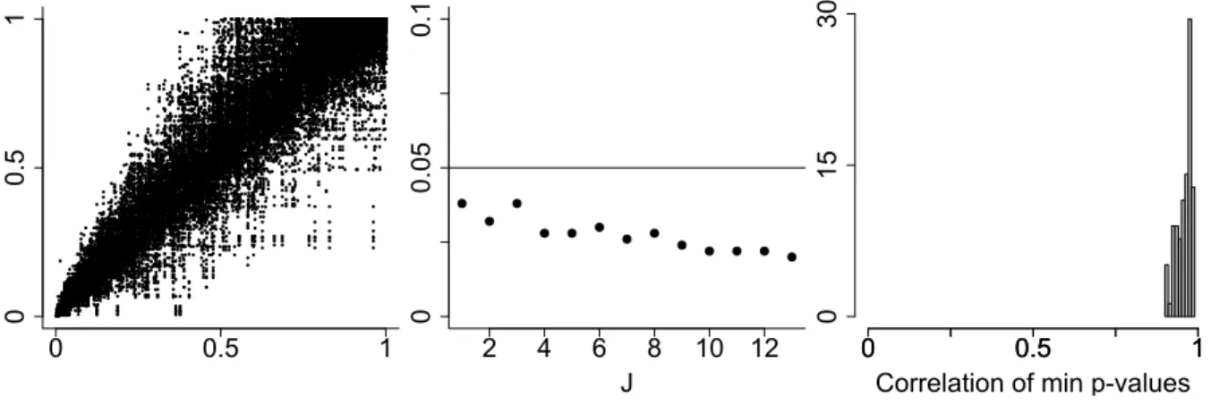
Simulation results from Section 4 confirm that Condition 6 appears to be satisfied in standard settings. We find Test (2) consistently obeys the α-limit due to individual undersizedness of Test (1) and nearly perfect dependence between grid-minimal p-values. Figure 1, which shows p-values of one specific setting, illustrates that both these points hold; results of other settings are in line, but not reported. We see that individual test sizes are consistently belowα, and decrease in the number of marginal hypotheses. Furthermore, correlation between minimal p-values of different grids is close to one, indicating nearly perfect (linear) dependence. Hence, we find Test (2) is appropriate.
Generally, it would be desirable to provide a lower bound of the strength of dependence between the p-values, i.e. a sufficient convergence rate in Con-dition 6. Convergence rates of individual test sizes and the unknown p-value dependence structure determine this lower bound. Unfortunately, to explicitly state this bound in our setting, we would have to assume specific closed-form distributions for the test statistics (Proschan and Shaw (2011)), or specific para-metric dependence model for the p-values, see Stange et al. (2015) and Bodnar and Dickhaus (2014). Yet, the precise dependence structure between the p-values is unknown, whereas tails of the test distributions may be approximated by χ2 distributions, see Beran (1975).
3.2
Local Tail Asymmetry
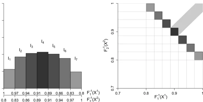
One main feature of our test is that we can localize tail dependence differences. This enriches the binary test decision on tail asymmetry/inequality as we can find subspaces in R2
+ where tail asymmetry/inequality can be expected. If the
global null is rejected, significant individual p-values trace the subsets of the unit simplex hull where both tail copulas differ. The boundary points of the significant subsets amount to empirical quantile threshold vectors which span
Figure 1: Exemplary p-values from the simulation study for Test (1) with j = 1, ...,13 (GARCH marginals equipped with a Factor model, k = 0.1n, n = 1500, tapered bootstrap). In this case, test size is estimated with 500 repetitions. Left: Scatterplots of p-values for all grid pairs. Middle: J, the fineness of the grids, is plotted against estimated test sizes according to Test (1). Right: Histogram of estimated correlations between all pairs of grid-minimal p-values.
0 0.5 1 0 0.5 1 2 4 6 8 10 12 J 0 0.05 0.1 0 0.5 1 0 0.5 1 0 15 30
Correlation of min p-values
a tail asymmetric subspace in the sample space, i.e.
QX=F1−,1 X(1−k/nx (1)), F−1 1,X(1−k/nx (2))×F−1 2,X(1−k/nx (1))), F−1 2,X(1−k/nx (2)), QY= F1−,Y1(1−k/nx(1)), F1−,Y1(1−k/nx(2)) ×F2−,Y1(1−k/nx(1))), F2−,Y1(1−k/nx(2)) .
Due to the homogeneity of the tail copulas, these extreme sets can be extrap-olated arbitrarily far into the tail, given the extreme value conditions hold. In particular, Figure 2 illustrates how to trace tail asymmetry.
Thus, when comparing tail dependencies of return vectors, our test pro-vides precise information on which specific tail events, or VaR events, cause tail dependence differences. Conditional on realized returns ofX(Y)falling into
QX (QY), tail dependence of X and Y differ; conditional on X(Y) ∈/ QX (QY), ΛX
and ΛY do not differ significantly.
This additional information might improve tail risk anticipation for regula-tors, or tail risk-based hedge and trading strategies for investors as those mar-ket times are identified which typically induce behavior of bivariate extremes to shift.
Figure 2: Left and right: Upper-right quadrants of scatterplots for X,Y, both
equipped with an asymmetric logistic copula and marginal distributions X(i) ∼
t(df = 3), Y(i) ∼t(df = 10), i = 1,2. The corresponding tail copula is Λ(x(1), x(2)) =
x(1) +x(2) −
(1− ψ(1))x(1) + (1− ψ(2))x(2) + ((ψ(1)x(1))−θ + (ψ(2)x(2))−θ)θ
(see Tawn (1988)), with parameters (ψ(1), ψ(2), θ) = (0.1,0.6,0.1), (ψ(1), ψ(2), θ) = (0.1,0.5,0.4). The shaded rectangles show the tail asymmetric tail regions; the homogeneity of the tail copula allows to extrapolate this region far into the sample tail. Center: Estimated tail copulas for x(1) ∈ {0.01,0.02, ...,0.99}, k = 500, n= 10000, M = 8. The shaded area indicates over which subset both tail copulas significantly differ.
0 4 8 12 X1 0 4 8 12 X2 L ^ (x1 , x2 ) 0 0.1 0.2 0.3 x1 0 0.5 1 0 4 8 12 Y1 0 4 8 12 Y2
4
FINITE SAMPLE STUDY
4.1
Serially Dependent Data
In general for financial time series, the i.i.d. assumption (A1) cannot be fulfilled as financial data typically exhibit strong serial dependence. Though, standard extreme value theory and the multiplier bootstrap rely on the independence assumption. We therefore consider two different approaches to address this problem.
The standard applied approach is to fit an appropriate time series speci-fication, such as e.g. ARMA-GARCH, to the financial raw returns and work with obtained standardized residuals. For a valid time series pre-filter, the lat-ter should roughly resemble an i.i.d. series, and can thus be used for further inference (see, e.g. McNeil and Frey (2000) in the univariate case). It is in-tuitively clear, that asymptotically such parametric pre-whitening at rate √n
should not affect rate and consistency of the slower converging nonparametric tail dependence estimates and thus of the test statistics. In practice, however, the pre-step might still lead in particular to second order effects in the variance for finite samples. In the following subsection we show that such effects are negligible for our test at considered standard sample sizes.
For empirical copulas of dependent data, another remedy is to assume sta-tionarity coupled with appropriate mixing conditions, which consequently allow to directly use unfiltered returns for estimation. Valid statistical inference is ensured by adjusting the bootstrap procedure: For strongly mixing time series, convergence of the block bootstrap and the so-called tapered block multiplier bootstrap has been shown for the empirical copula process, Bücher and Rup-pert (2013). Necessary assumptions are met for a wide class of time series models, such as ARMA and GARCH models. We suggest to use the dependent data bootstrap methodology also for empirical tail copulas.
We therefore replace the iid multipliers with a dependent multiplier sequence defined as follows
Assumptions 2.
(A6a∗) The tapered block multiplier process (ξj,n)j=1,...,n is strictly stationary with
E[ξ0,n] = 0, E[ξ02,n] = 0 , and E[|ξ0,n|ν] < ∞ for all ν ≥ 1 independent of
Z1, . . . ,Zn.
(A6b∗) For any j, ξj,n is independent ofξj+h,n for all h ≥ l(n) where l(n) is a strictly
positive, deterministic sequence withl(n)→ ∞and l(n) = O(n).
(A6c∗) For any h ∈ Z, there exists v : R → [0,1] such that E(ξ0,n, ξh,n) = v(h/l(n))
where v continuous at 0 and symmetric around 0 withv(0) = 1 andv(x) = 0 for |x|>1.
Instead of the i.i.d. Assumption (A1) the underlying stochastic process
Z ∈ {X,Y} is required to be strictly stationary and αZ-mixing with αZ(r) =
αZ(Fs,Fs+r) = supA∈Fs,B∈Fs+r|P(A∩B)−P(A)P(B)|,for the(Z1, . . .Zt)-induced
filtra-tionFt. The rate of decayαZ(r) = O(r
−aZ)wherea
Z >0forr >0marks the degree
of admissible serial dependence. In contrast to standard copulas, weak conver-gence of empirical tail copulas in an α-mixing set-up is a challenging problem which has only been touched upon very recently in special cases so far, see e.g. Bücher and Ruppert (2013) and Bücher and Segers (2017). A general proof is beyond the scope of this paper, however, the later paper suggests, that this is possible under fairly general conditions in our bivariate set-up, in particular allowing for processes of ARMA-GARCH-type which are key to financial appli-cations. For the case aZ > 6, Bücher and Kojadinovic (2016) show a general multiplier bootstrap theorem for dependent data and multipliers of the type as in Assumption 2 for the case of standard copulas. This is key for formally deriving the consistency of the tapered multiplier bootstrap with block length
l(n) → ∞, where l(n) = O n1/2−,0 < < 0.5., but the theoretical extension to tail copulas is non-trivial and left for future research.
We construct the tapered multiplier bootstrap with a dependent multiplier series as in Assumption 2 entering both empirical copula and marginal empiri-cal distribution in (5). In each bootstrap roundb, these yield the tapered version
of test statisticSbm,(b),tap by plugging them into equation (4), from which the final b
Sm,?,tap can be constructed for eachm = 1, . . . , M.
For the choice of multiplier block length l under which the generated mul-tiplier series mimics the resulting dependence structure of Z we follow Bücher and Ruppert (2013) in their implementation guidelines setting l(n) = 1.25n1/3.
Moreover, for the tapered block multiplier bootstrap, we employ the uniform kernel κ1, and use Γ(q, q)-distributed base multipliers, with q = 1/(2l(n)− 1),
where l(n) is the multiplier block length, which can be automatically deter-mined using from the R-package npcp, see Kojadinovic (2015). Our compre-hensive simulation study underlines the validity of the tapered multiplier boot-strap for the empirical tail copula, suggesting thatSbm,?,tap w→Sm form = 1, . . . , M.
With this approach the tail dependence structure is not polluted due to poten-tial model misspecification from pre-filtering which may be a problem for large, high-dimensional data sets where automatic GARCH fitting is challenging and computationally expensive.
4.2
Simulations
We now compare the finite sample performance of our test with the TDC test, and the BD13 test. We focus on non-parametric tests as in practice parametric specifications may suffer from a model bias, especially if intra-tail asymmetry is not accounted for. We study two types of dependence models that are frequently used in finance. First, we employ the (implicit) factor model copula. See Fama and French (1992), Einmahl et al. (2012), and Oh and Patton (2017) for factor models in finance, tail dependence of factor models, and tail dependence of factor copulas in finance, respectively. Second, representing the broad class of Archimedean copulas, we employ the Clayton copula, which models solely lower tail dependence. Its lean parametric form makes the Clayton copula a popular building block for more complex copula models, such as mixtures of copulas, see Rodriguez (2007) and Patton (2006). For each copula, we impose one parametrization that fulfills the null, and one that violates the null, leaving
us with four DGPs.
DGP1 and DGP2 are based on the tail factor model. Bivariate return vectors
Z = (Z(1), Z(2)),Z = X,Y, follow a bivariate factor model with r factors V(j), j = 1, ..., r,and loadings aij, i= 1,2, j = 1, ..., r, when
Z(i) =
r
X
j=1
aijV(j)+ε(i), i= 1,2, (7)
where factors are i.i.d. Fréchet with ν = 1, independent of the error term ε(i)
which feature thinner tails than V(j); we set ε(i) as Fréchet with ν
ε = 2. In this
way, the matrix of factor loadings A = (aij) directly determines the tail copula
of Z. In particular, the (upper) tail copula ofZis equivalent to the tail copula of the max factor model Z¯(i) = max
j=1,...,r(aijV(j)), which is ΛU(x(1), x(2)) =x(1)+x(2)− r X j=1 max Pra1j j=1a1j x(1),Pra2j j=1a2j x(2) ! ,
see Einmahl et al. (2012) for further details. DGP1 consists of X,Yboth result-ing from a factor model as in Equation (7), but with loadresult-ing matrix
A1 = [2 1 00 1 2].
Here, the first factor only influences X(1) (Y(1)), the second factor influences
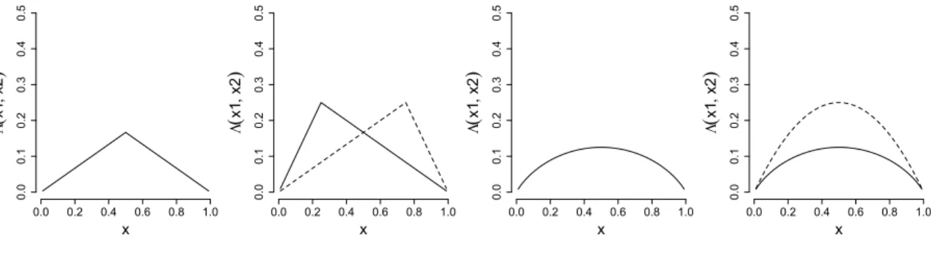
both X(1) (Y(1)) and X(2) (Y(2)), and the third factor only influences X(2) (Y(2)). That is, A1 amounts to intra-tail symmetry and to tail equality betweenXandY,
and thus the null is true. See Figure 3, first from the left, for Λ(x(1),1−x(1)), x(1) ∈
[0,1]. For DGP2, both X and Ystem from a factor model as in Equation (7) with
A2 = [1 01 2],
where the second factor only influences X(2) (Y(2)), causing the tail copula to become intra-tail asymmetric, Λ(x(1), x(2)) 6= Λ(x(2), x(1)), and consequently tail
Figure 3: Tail copulas of DGPs 1 to 4 from left to right. Note, for DGP2, the solid lines represents Λ(x(1), x(2)), x(2) = 1−x(1), whereas the dashed line shows
Λ(x(2), x(1)). For DGP4, two different specifications of the Clayton copula are
used for X and Y.
x L ( x1 , x2 ) 0.0 0.1 0.2 0.3 0.4 0.5 0.0 0.2 0.4 0.6 0.8 1.0 x L ( x1 , x2 ) 0.0 0.1 0.2 0.3 0.4 0.5 0.0 0.2 0.4 0.6 0.8 1.0 x L ( x1 , x2 ) 0.0 0.1 0.2 0.3 0.4 0.5 0.0 0.2 0.4 0.6 0.8 1.0 x L ( x1 , x2 ) 0.0 0.1 0.2 0.3 0.4 0.5 0.0 0.2 0.4 0.6 0.8 1.0
the left. DGP2 thus represents the class of intra-tail asymmetric copulas which violate the null according to Proposition (1).
For the Clayton copula, only the lower left part of the distribution features tail dependence,
ΛL(x(1), x(2);θ) = (x(1)−θ+x(2)−θ)−1/θ,
ΛU(x(1), x(2);θ) = 0,
where (lower) tail dependence increases in the parameter θ ∈ [0,∞). DGP3 is given by X,Y ∼ Clayton(θ = 0.5); this specific choice of θ implies a TDC
of ι = 0.25, which roughly corresponds to a TDC of a bivariate t-distribution with correlation 0.5 and four degrees of freedom (McNeil et al. (2005), p.211). For DGP3, the null is true. See Figure (3), second from the right. For DGP4,
X ∼ Clayton(θ = 0.5), and Y ∼ Clayton(θ = 1). Thus, tail equality is violated as
the TDC of Y isι= 0.5. See Figure (3), first from the right.
To check whether the test also works for financial time series data, we com-bine all DGPs with i.i.d. as well as GARCH marginals. We apply the test to raw
GARCH returns, and to standardized GARCH residuals as it is important to an-alyze whether usingestimated residuals affects test performance. Moreover, we study the test performance for unfiltered returns using the block bootstrap and
the tapered block multiplier bootstrap. In particular, we employ GARCH(1,1) dynamics for any marginal return process. We follow Oh and Patton (2013) and employ bivariate AR-GARCH models. We can link serially dependent marginals by the (implicit) copulas of DGPs 1 to 4, allowing us to study the effect of condi-tional heteroscedasticity on test performance. For both bivariate return series
Z= (Z(1), Z(2)),Z=X,Y, it holds Zt(i) =σt(i)η(t,i) Z, σt,2,(i) Z =ω+α (i)Z(i) t−1+β (i)η2,(i) t−1,Z, ηZ := (η(1) Z , η (2) Z )∼iid Fη,Z(x (1), x(2)) =C η,Z(Fη,Z,1(η (1) Z ), Fη,Z,2(η (2) Z )), t= 1, ..., nZ,
where we set ω = 0.01, α = 0.15 and β = 0.8 such that ω + α +β is close to one. This mimics parameter values often found in financial returns, see for example Engle and Sheppard (2001). To impose the tail structures of DGPs 1 to 4 on the time series, we use DGPs 1 to 4 to model the error copula
Cη,Z(Fη,Z,1(η (1)), F η,Z,2(η (2)))and to generateη t,Z = (η (1) t,Z, η (2)
t,Z): In a first step, we
sim-ulate observations ηt,Z according to DGPs 1 to 4. Consequently, we transform
simulated errors to pseudo-observations by means of the marginal empirical cumulative distribution, Fbη,Z,i(η
(i)
t,Z), i = 1,2. Finally, we apply the quantile
func-tion of the t-distribution function with 10 degrees of freedom to the pseudo-observations. Thus, the final errors are linked by the copulas of DGPs 1 to 4 with fat-tailed t-marginals. Those are used to generate the GARCH series for X and Y, and standardized residuals obtained from estimation by quasi maximum likelihood. Note, monotone transformations, such as the quantile transformation, do not alter the tail dependence structure, and should not al-ter test results. However, t-transformed error distributions are a more realistic approximation of asset returns.
For sample sizes n = 750,1500, varying values of the effective sample size
k, and a nominal test level of α = 0.05, we compare empirical rejection fre-quencies. Also, for Test Algorithm ((1)), we employ two subset discretizations (M = 6,18) to evaluate the sensitivity of the test performance with regard to the
user-dependent test calibration. Furthermore, we employ Test Algorithm ((2)) which merges 15 different grids with grid sizes Mj = 2j, j = 1, ...,15,. For some
grids, this implies that subintervals are only roughly of equal length. The TDC test is carried out using the multiplier bootstrap at points x(1) = x(2) = 0.5. The
number of simulations is S = 500for each setting.
Table (1) reports empirical rejection frequencies for i.i.d. marginals, fil-tered GARCH marginals, unfilfil-tered GARCH marginals, GARCH marginals with the block and tapered bootstrap, and sample size n = 1500 while we refer to the online appendix for simulation results with n = 750; As non-parametric methods for tail dependence are often criticized for unsatisfactory small sam-ple performance, it is worth studying test behavior for small and moderate sample sizes. Also, we study the effect of varying the effective sample size,
k ∈ {b0.1nc,b0.2nc,b0.3nc}. Note, Λ(x(1), x(2);k =k∗) = Λ(ax(1), ax(2);k =ak∗). Hence, these values for k correspond to b0.05nc,b0.1nc,b0.15nc in the standard case of TDC estimation with x(1) =x(2) = 1.
In general, both Test ((1)) and Test ((2)) appear to be consistent. For i.i.d. marginals, both obey the nominal test size of α = 0.05 (DGP1 and DGP3), ir-respective of the choice of k. This is particularly important for Test ((2)) as it points out that grid-specific p-values appear to be sufficiently dependent to keep empirical size below α, although no additional multiplicity penalty is ap-plied. While empirical test size remains untouched by k, the choice of effective sample size notably affects empirical power; for example, for DGP4, power in-creases by up to 25% both for M = 6,18. Hence, this suggests a larger choice of
k is favorable. As noted in Bücher and Dette (2013), for a large k, bias terms in ΛbX and ΛbY cancel out. This suggests the choice of k, which in essence is
a bias-variance problem for Λb, is slightly facilitated compared to other extreme
value-based peaks-over-threshold problems. Thus,k≈0.1nseems a reasonable rule of thumb.
While single-grid tests (Test ((1))) show larger power than the TDC test, the BD13 test is more powerful in standard cases compared to Test ((1)). However,
combining a multiple of single-grid tests, e.g. Test Algorithm ((2)), makes our test consistently more powerful than BD13.
Importantly, our test successfully rejects in case of intra-tail asymmetries, as shown by the empirical rejection frequencies for DGP2. Both the TDC test and BD13 test fail to reject the null in this case and completely ignore intra-tail asymmetries. If the intra-tail copula is intra-asymmetric, our power of our tests increases in the number of employed subsets. If the tail copula is symmetric, however, power decreases in M. It is thus advisable to apply Test ((2)).
Also, test results for GARCH filtered returns are in line with i.i.d. series. The estimation step of the GARCH residuals does not downgrade neither test power nor size. However, unfiltered GARCH returns should not be used: In the case of DGP4, test power implodes by roughly 50−75% for all three tests. Empirical sizes for DGP1 are still fine, whereas empirical size of DGP3 generally is too large.
The tapered block multiplier bootstrap produces results comparable to the multiplier bootstrap-based on i.i.d. and GARCH filtered marginals. Thus, we prefer a bootstrap adjustment over GARCH-filtering to address serial depen-dence it can handle serially dependent data and does not require pre-estimation of a parametric model. However, as Table (1 Appx) in Appendix B of the online supplement suggests, the tapered block bootstrap should only be applied for larger sample sizes, since for n = 750 and GARCH marginals the tapered mul-tiplier block bootstrap appears to be oversized and hence GARCH-filtered data should be used instead.
Finally, we find our aggregating test (Test ((2))) is throughout most powerful, while the test with fixed grids (Test ((1))) is consistently more powerful than the TDC test, slightly less powerful than the BD13 test, and more powerful than the latter in case of intra-tail asymmetry.
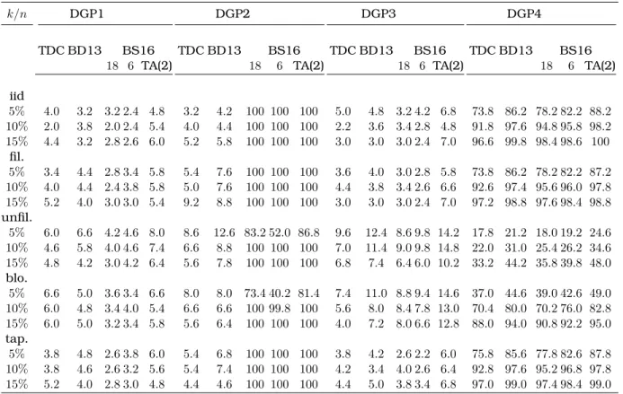
Table 1: Empirical rejection probabilities for α = 5%, S = 500 repetitions and sample size n = 1500. Effective sample fraction k/n is evaluated at
(x(1), x(2)) = (1,1). DGP1: factor model satisfying H
0. DGP2: factor model
violat-ing H0. DGP3: Clayton copula satisfying H0. DGP4: Clayton copula violating
the null. Rejection frequencies are shown for a varying effective sample size, i.i.d. marginals and GARCH marginals for which the tests are applied to raw observations (unfiltered) and also to standardized residuals (filtered). For the latter, estimation was carried out by quasi maximum likelihood.
k/n DGP1 DGP2 DGP3 DGP4
TDC BD13 BS16 TDC BD13 BS16 TDC BD13 BS16 TDC BD13 BS16
18 6 TA(2) 18 6 TA(2) 18 6 TA(2) 18 6 TA(2)
iid 5% 4.0 3.2 3.2 2.4 4.8 3.2 4.2 100 100 100 5.0 4.8 3.2 4.2 6.8 73.8 86.2 78.2 82.2 88.2 10% 2.0 3.8 2.0 2.4 5.4 4.0 4.4 100 100 100 2.2 3.6 3.4 2.8 4.8 91.8 97.6 94.8 95.8 98.2 15% 4.4 3.2 2.8 2.6 6.0 5.2 5.8 100 100 100 3.0 3.0 3.0 2.4 7.0 96.6 99.8 98.4 98.6 100 fil. 5% 3.4 4.4 2.8 3.4 5.8 5.4 7.6 100 100 100 3.6 4.0 3.0 2.8 5.8 73.8 86.2 78.2 82.2 87.2 10% 4.0 4.4 2.4 3.8 5.8 5.0 7.6 100 100 100 4.4 3.8 3.4 2.6 6.6 92.6 97.4 95.6 96.0 97.8 15% 5.2 4.0 3.0 3.0 5.4 9.2 8.8 100 100 100 3.0 3.0 3.0 2.4 7.0 97.2 98.8 97.6 98.4 98.8 unfil. 5% 6.0 6.6 4.2 4.6 8.0 8.6 12.6 83.2 52.0 86.8 9.6 12.4 8.6 9.8 14.2 17.8 21.2 18.0 19.2 24.6 10% 4.6 5.8 4.0 4.6 7.4 6.6 8.8 100 100 100 7.0 11.4 9.0 9.8 14.8 22.0 31.0 25.4 26.2 34.6 15% 4.8 4.2 3.0 4.2 6.4 5.6 7.8 100 100 100 6.8 7.4 6.4 6.0 10.2 33.2 44.2 35.8 39.8 48.0 blo. 5% 6.6 5.0 3.6 3.4 6.6 8.0 8.0 73.4 40.2 81.4 7.4 11.0 8.8 9.4 14.6 37.0 44.6 39.0 42.6 49.0 10% 6.0 4.8 3.4 4.0 5.4 6.6 6.6 100 99.8 100 5.6 8.0 8.4 7.8 13.0 70.4 80.0 70.2 76.0 82.8 15% 6.0 5.0 3.2 3.4 5.8 5.6 6.4 100 100 100 4.0 7.2 8.0 6.6 12.8 88.0 94.0 90.8 92.2 95.0 tap. 5% 3.8 4.8 2.6 3.8 6.0 5.4 6.8 100 100 100 3.8 4.2 2.6 2.2 6.0 75.8 85.6 77.8 82.6 87.8 10% 3.8 4.6 2.6 3.2 5.6 5.4 7.4 100 100 100 4.2 3.4 4.0 2.6 6.4 92.8 97.6 95.2 96.8 97.8 15% 5.2 4.0 2.8 3.0 4.8 4.4 4.6 100 100 100 4.4 5.0 3.8 3.4 6.8 97.0 99.0 97.4 98.4 99.0
5
TAIL ASYMMETRIES IN THE US STOCK MARKET
Related studies, e.g. Ang and Chen (2002), focus on tail asymmetries in pairs of international stock indices, and point out that, especially during financial crises, correlations mainly between extreme losses increase. We are inter-ested whether this finding also applies for sector pairs in the US stock market. Hence, we study possible tail asymmetries between daily returns of 49 US in-dustry sectors. The dataset, available at http://mba.tuck.dartmouth.edu/ pages/faculty/ken.french/data_library.html, accessed on 03/01/2016, contains nearly 90 years of weighted returns of CRSP SIC codes-based indus-tries of NYSE, AMEX, and NASDAQ stocks. Fama and French (1994) and Chang et al. (2013) analyze earlier versions of this dataset.
We proceed as follows. We aim to detect tail asymmetry dynamics within the US stock market. Applying a rolling window analysis with window length of
n = 1500, i.e. nearly six years, and a step size of 250 trading days, i.e. roughly
14 months, we arrive at 74 (overlapping) time periods. In each period, we build all possible bivariate industry combinations ,X= (X(i), X(j)), and test the nulls
H0 : ΛUX = ΛLX.
Discarding pairs with missing data, in each period, there are at most1176 pairs to test against tail asymmetry. In total, we apply the test approximately 85,000
times. To avoid possible model risk by pre-filtering the returns, we throughout analyze raw returns using the tapered block multiplier bootstrap; Section 4.1 and the results of the simulation study justify this approach. For completeness, however, we also computed results from GARCH pre-filtering. As there are only minor differences to the results from tapered bootstrap we only provide them in Appendix C of the Web-Appendix. We set the window parameter of the tapered block multiplier bootstrap to l = 8. Yet, we find no change of results worth mentioning when altering l. Also, we fix the effective sample size to
not interested in particular industry pairs as our focus is on tail asymmetry of the general market. Hence, a fixed k for all pairs is an operable solution to the question of number of extremes as over- and underestimation might eventually balance out when aggregating test decisions over all1176pairs. Note, this section studies tail asymmetries. In the online appendix, we also provide an empirical study on tail inequalities between foreign exchange rates.
To grasp the general evolution of lower and upper bivariate tails, we intro-duce a descriptive measure for upper and lower market tail dependence. In period t, for each pair i, we integrate the empirical tail copula Λbi(φ,1−φ) over
[0,1]and provide empirical location statistics across all pairs, e.g. the mean and empirical quantiles. For the mean,
Λt := 1 nt 2 (nt 2) X i=1 Z 1 0 b Λi(φ,1−φ)dφ,
where nt is the number of sectors in period t, and empirical quantiles are
com-puted accordingly. It is easy to see that R1
0 Λ(φ,1−φ)dφ ∈ [0,0.25]. The lower
(upper) bound is attained if pair i has no (perfect) tail dependence. Figure (4) shows the trajectory of the mean and q-quantiles, q ∈ {0.01, ...,0.99}, for both upper and lower tails covering 1931 - 2015.
The null hypothesis of tail equality is tested by the TDC test, the BD13 test and Test ((2)), which aggregates over 15 grids in the spirit of the simulation study. Figure 5 displays trajectories of the share of rejections for each test, i.e. the share of tail asymmetric pairs according to each test. Figure 6 documents the importance of non-standard tail events, i.e. non-TDC events that occur off the diagonal (x(1) =x(2)).
All tests indicate that most of the time, a substantial amount of tail asymme-tries exists in the market. We find that our test reveals more tail asymmeasymme-tries than competing tests which we attribute to non-diagonal tail dependence and intra-tail asymmetry. Furthermore, we find tail asymmetry typically vanishes during financial crises, expect for the subprime crisis when tail asymmetries
occurred more frequently than shortly before and afterwards. This finding may reflect the classical risk-return traoff with a new livery: As lower tail de-pendence, i.e. the risk of joint extreme losses, spikes during financial distress, opportunities for joint extreme gains must counteractively increase as we detect more tail asymmetries during bear markets.
On average, our test finds that 64% (sd=0.25) of all pairs exhibit tail asym-metry. We can identify a long lasting phase of pronounced tail asymmetries between 1940-70 where on average 80% (sd=0.10) of all pairs are tail asym-metric. Collapses of the number of tail asymmetries strikingly coincide with of financial crises, such as the beginning of the Great Depression (1932-37), the Oil Crisis (1968-74 until 1972-78), Black Monday (1987) and the Asian and millennium crisis accumulating into the Dot-Com crisis (1995 - 2003). It is empirically documented that in crises losses increasingly move in extreme ways. We can only conclude that, during crises, the tendency of extreme gains to co-move also increases. The latter might compensate investors for facing extreme downside risk in large cross-sections. That is to say, when bivari-ate losses occur more frequently, one can also expect more bivaribivari-ate extreme gains. In contrast, the recent financial crisis 2007-09 is characterized by a temporary bump in tail asymmetries which subtends a phase of steady decline of tail asymmetries since the mid 1990s. One might argue that, in contrast to former financial crises, only tail dependence between losses was affected. But tail dependence between gains did not experience such change. This makes the subprime crises particularly disastrous as investors did not encounter much extreme upside potential. However, aggregated tails of the market (Figure 4) hardly back this conclusion as we observe a nearly parallel progression of both upper and lower tail measures. Thus, by aggregating bivariate tails to an index measure, much information on the tail dependence between tails of the index’ constituents is lost. While the summary measures for market tail dependence suggest left and right tails are connected equally strongly during the 2000s, all three tests report otherwise and reveal a pattern not captured by descriptive
statistics. This implies tail measures for indices do not tell the same story their constituents can.
In comparison to the two competing tests, our test consistently detects more asymmetries, see Figure 6 (left), which we attribute to the fact that competing tests overlook non-central tail dependence structures (TDC test), or intra-tail asymmetry (TDC test, BD13 test). Hence, our test provides a more accurate assessment of tail asymmetry within the market and suggests tail asymmetry is more common than expected. With respect to the TDC test (BD13 test), we find2.5%−27% (0%−12%)more tail asymmetric pairs. We also plot the trajectory of the percentage of rejections where, for Test (1) with M = 14, the adjusted p-value of the central subinterval does not suggest a rejection, while at least one non-central p-value does (solid line, Figure 6). This line runs nearly parallel to the graph of the differential in found tail asymmetries between the TDC test and our test.
To further underline the importance of non-standard tail dependence struc-tures, we quantify the number of tail asymmetric pairs that scalar approaches would miss due to off-diagonal tail asymmetries. In Figure 6 (right), for each period, we compare the number of rejections of non-central subintervals with the number of rejections found in the central subinterval. We find that our test, when restricted to non-diagonal subintervals, finds up to 20% more asymme-tries than a TDC-based analysis that solely focuses on the central subinterval. Throughout the sample, there exists at least one non-central subinterval with more test rejections than the central subinterval. Furthermore, there are peri-ods of time – which match the major financial crises – where not considering off-diagonal parts of the TC is especially serious. Yet, in the finance literature, e.g. Jondeau (2016), it is common practice to analyze tail dependence solely by the tail dependence coefficient ι, i.e. the tail copula along the diagonal where
x(1) =x(2). We document that this approach might overlook non-standard types
of tail dependence leading to a substantial misconception of tail asymmetry. A more detailed picture of the local impact on tail asymmetry is provided in Figure
7 which marks rejection frequencies for specific quantile regions as discussed in Subsection 3.2. This could directly translated into investment and hedging strategies.
Furthermore, the difference in found asymmetries between our test and BD13 suggests some degree of intra-tail asymmetry among all pairs. The simulation study demonstrated both tests’ power differs mainly in intra-tail asymmetric cases. Applying tests against intra-tail symmetry (Kojadinovic and Yan (2012); Bormann (2016)), we quantify the importance of intra-tail asym-metries for tail asymasym-metries. Both test check the (tail) copula against non-exchangeability with Cramér-von Mises tests, while the latter tests explicitly accounts for serial dependence, and is thus more appropriate here. We use a significance level of α = 0.05. For periods with the smallest and the largest dis-crepancy in the number of test rejections between our test and the BD13 and the TDC test, respectively, we test for intra-tail asymmetries. Table 2 contains the test results. Intra-tail asymmetry of a sector implies one sector’s extremes are more likely to trigger extreme events of the other sector. This demands special care in hedging as anticipation of (conditional) extremes is uneven. For small (large) discrepancies, we expect no (a) significant portion of test rejec-tions. When our test does not find substantially more tail asymmetries than BD13 during 1975–81 (TDC during 1977-83), we detect only 4.1% (3.5%) intra-tail asymmetric pairs. On the other hand, this share rises to 12.5% (9.13%) when our test is more powerful with respect to detecting tail asymmetry (BD13 during 1938–1943, TDC during 1945–51). Although the share of found intra-tail asymmetries is relatively small, this supports the conjecture that intra-intra-tail asymmetry explains the differences in test results.
Figure 4: R1
0 Λ(b x,1−x)du for all possible pairs (up to 1176) in each period; dark
line: empirical mean; gray lines: empirical quantiles: 0.01i, i = 1, ...,99. Left: losses. Right: gains.
0.00 0.05 0.10 0.15 0.20 0.25 ó õ0 1^L L(u,1-u)du 1931 1941 1953 1965 1978 1990 2003 2015 0.00 0.05 0.10 0.15 0.20 0.25 ó õ0 1^L U(u,1-u)du 1931 1941 1953 1965 1978 1990 2003 2015
Table 2: ITA test results. We test against ITA in periods when results of our test and competing tests are most (least) similar, i.e. when the shares of test rejections is the largest (the closest). See also Figure 5. In such periods, we report the share of bivariate tails that the test identifies as intra-asymmetric.
BD13 TDC
test results period ITA period ITA
similar
1975-81 4.1% 1977-83 3.5%
maximally different