Weld Defect Detection using Ultrasonic Phased Arrays

(1)

Weld Defect Detection using Ultrasonic Phased

Arrays

by

Bryan Cassels

A thesis submitted in partial fulfilment for the requirements for the degree of Doctor of Philosophy at the University of Central Lancashire

in collaboration with BAE Systems Maritime

(2)

STUDENT DECLARATION FORM

Type of Award Doctor of Philosophy School Engineering

1. Concurrent registration for two or more academic awards

I declare that while registered as a candidate for the research degree, I have not been a registered candidate or enrolled student for another award of the University or other academic or professional institution

2. Material submitted for another award

I declare that no material contained in the thesis has been used in any other submission for an academic award and is solely my own work

3. Collaboration

Where a candidate’s research programme is part of a collaborative project, the thesis must indicate in addition clearly the candidate’s individual contribution and the extent of the collaboration. Please state below:

The project is in collaboration with the sponsor BAE Systems Maritime. They have provided funding, access to experimental facilities and advice. However, all the work in this thesis is from my own investigations and evaluations.

4. Use of a Proof-reader

No proof-reading service was used in the compilation of this thesis.

Signature of Candidate

(3)

Abstract

Many traditional ultrasonic test methods, based on the manipulation of an ultrasonic probe by an experienced inspector, are beginning to be replaced by Automated Ultrasonic Testing (AUT). Largely limited to regular structures, the integration of phased arrays and computer controlled mechanical manipulators allows AUT to provide fast, regular and repeatable data acquisitions for off-line inspection and future auditing. The objective of this thesis is to investigate methods of assisting with the inspection of these vast quantities of data. To this end the emphasis is on detecting regions of a weld that do not comply to the normal, anomaly free, structure.

It is found that a multivariate analysis, using Principal Component Analysis (PCA), im-proves the Probability Of Detection (POD) of anomalies over univariate techniques, which rely on only the segmentation of regions with unusually high ultrasonic reflections. A further finding is that the multivariate approach is capable of mitigating the effects of dominating front wall reflections and other continuous features.

Experimental results using test block data reveal a high POD with a low false alarm rate. This is particularly the case where the probe is in direct contact with the test piece and the front wall is gated out. Despite a lower POD the immersion results are particularly significant in that they permit the use of segmentation procedures simply not possible in the univariate case.

Although limited to 2D anomaly location it is relatively straightforward, using the 2D location as a key, to extract full volumetric data of the anomaly from the original 3D

ultrasonic data set. A future extension of this work is to use the 3D information to

accurately classify any anomaly. In addition to providing a more detailed description of the anomaly this also has the potential to reduce the false alarm rate.

AUT produces vast quantities of data for inspection. It is increasingly common for this data to be in the form of a sequence of images representative of a weld’s cross section. Manual inspection of each image, by qualified personnel, is both expensive and prone to human error. The system developed here has the potential to improve this process by considerably reducing inspection time, and cost, whilst maintaining a consistently high POD.

(4)

Acknowledgements

I would first like to give my thanks to my supervisors Lik-Kwan Shark and Stephen Mein without whose help much of the work presented in the thesis could not be done. They both provided inspirational ideas with valuable insights and continual enthusiasm.

Sincere thanks are also expressed to Tom Barber, Andrew Nixon and Ray Turner for their valuable advice. In addition to giving considerable encouragement throughout the entire programme they also helped with experiments and provided data without which, this work would largely contain only simulations.

For project funding acknowledgement and thanks must be given to BAE Systems Maritime. Finally I must give thanks to my wife, Pat, for her endless patience, encouragement and support. Not forgetting Dylan and Rosie who remind me of the important sides to life.

Bryan Cassels August 2018

(5)

8.10.5.1 Additional thresholding . . . 243 8.10.6 Blob detection . . . 243 8.10.6.1 Sparse matrix . . . 246 8.10.7 Chapter summary . . . 250 9 Conclusions 256 9.1 Contribution to knowledge . . . 258 9.2 Further work . . . 259 9.3 Industrial impact . . . 260 Appendices 262 A Delay and sum beam forming 263 A.1 Delay and sum beam forming . . . 263

B Snell’s law derivation 266 B.1 Snell’s law . . . 266

(11)

Abbreviations

ADMM Alternating Direction Method of Multipliers

AUC Area Under Curve

AUT Automated Ultrasonic Testing

BIP Beam Intersection Point

FAR False Alarm Rate

FN False Negative

FP False Positive

FBH Flat Bottomed Hole

FMC Full Matrix Capture

GT Ground Truth

HDLSS High Dimensional Low Sample Size

KI Kittler and Illingworth (Minimum error thresholding)

LOF Local Outlier Factor

MCD Maximum Covariant Determinant

MCE Miss-Classification Error

MCC Mathews Correlation Coefficient

ME Maximum Entropy (thresholding)

MVE Maximum Volume Ellipsoid

(12)

NPD Negative Predictive Value

PA Phased Array

PC Principal Component

PCA Principal Component Analysis

PCP Principal Component Pursuit

POD Probability Of Detection

ROC Receiver Operating Characteristic

RPCA Robust Principal Component Analysis

SAFT Synthetic Aperture Focusing Technique

SBH Spherical Bottomed Hole

SDH Side Drilled Hole

SNR Signal to Noise Ratio

TB Test Block

TFOCS Templates for First Order Conic Solvers

TN True Negative

TP True Positive

(13)

Chapter 1

Introduction

Welding is perhaps the most widely used method of joining together metals and alloys. Since the beginning of the 20th century with the formation of organisations such as the American Welding Society, documented research into welding has continued to accelerate. A significant result is the development of numerous processes and methods of automation. Today many techniques exist that are capable of efficiently and continuously producing welds with a high degree of reliability. Similarly quality assurance techniques are mature and encompass control of the whole process. For example BS EN ISO 3834 [1] sets out requirements of weld quality for manufacturers to meet; BS 3923-1 [2] sets out methods of inspection, whilst standards such as Defence Standard 02-773 [3] apply to specific envi-ronments. Conformance to these standards comes at considerable expense through the use of highly qualified personnel and time. Justification is that the effect of just a single weld failure can be catastrophic. For example when many large structures (ranging through buildings, bridges, dams, pipelines, ships’ hulls, aircraft, nuclear power plants and power generator boilers) depend on the integrity of their welds, a single failure has potential for high monetary costs, damage to the environment or loss of human life [4], [5]. Consequently the expectation of weld quality has never been higher.

Following visual examination of a weld, one of the earliest forms of Non Destructive Testing (NDT) was the use of a liquid penetrant dye [6]. The earliest test, known as the ‘Oil and

Whitting Method’, was introduced in the late 19th century. However it was not until

shortly after the sinking of the Titanic in 1912, that the roots of modern NDT and Non Destructive Evaluation (NDE) began to be established [5]. In the 1940’s the accepted standard of inspection for critical structural welds was, according to DeNale and Lebowitz [7], radiography. They also record that the gradual introduction of ultrasonic inspection,

(14)

for similar applications, only started in the early 1960’s. Over much of the intervening time radiography remained, for safety critical applications, the preferred method.

In principle, the radiographic test procedure is straightforward. On one side of the weld is a film (or more recently an electronic detector) and on the other is the source of radiation. As the beam of radiation passes through the weld, its interaction with anomalies causes higher levels of attenuation than does that through the more homogeneous, anomaly free, background. After developing, the film contains an image of the weld, and its surrounding area (figure 1.1). This provides a permanent record of the weld’s internal structure. It can (depending on film’s size) cover a long length of weld. To distinguish this type of projection onto film, from that of a photograph produced by light, the image is known as a radiograph.

There are, however, a number of difficulties with radiography, the most serious being due to radioactivity. Not only must strict health and safety rules be followed during operation but an entire work area may need to be evacuated before tests begin and for a period afterwards. This is costly in terms of lost production. In addition to this expense other limitations of radiography are that it is highly directional, sensitive to the orientation of a flaw, does not indicate the depth of the flaw and requires a high degree of skill and experience for exposure and interpretation [7].

Figure 1.1: Example of a radiographic recording (from www.nde-ed.org)

Ultrasonic inspection using a single element probe does not suffer from these health and

safety limitations. Through a sequence of adaptive closed loop manual operations an

inspector, through skill and experience, is able to detect and reliably sentence any anomaly within the weld. However such approaches remain time consuming, full coverage of the weld is at the discretion of the inspector and there is no record of the ultrasonic data for future auditing purposes.

(15)

1.1 Industrial application

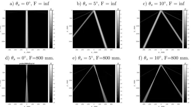
In the early 1960’s researchers started to develop ultrasonic phased arrays. In contrast to the single element probe these initially contained a line of small equally spaced point sources. As each element requires a dedicated channel to excite and record the response from each ultrasonic element, complete systems were large and expensive. Continuing developments in micro-electronic lithography meant that, starting around the 1990s, low power CMOS technology had developed to the extent that inexpensive and portable multi-channel phased array systems were gaining in popularity. A significant advantage of these systems over single element probes is their ability to apply a timed sequence of pulses to individual elements. This allows the ultrasonic beam to be steered and focused, as in the case of a sectorial scan. Alternatively it is possible to create an image through a process of synthetic focusing at each pixel point in an image. Examples of this are the Synthetic Aperture Focusing Technique (SAFT), [8] and the Total Focusing Method (TFM), [9].

a) Sector Scan b) TFM Image

20 40 60 80 100 120

Offset (pixel no.)

20 40 60 80 100 120

Depth (pixel no.)

-40 -35 -30 -25 -20 -15 -10 -5 0 db Water Specimen Weld cap Anomaly

Figure 1.2: Example cross sectional images using a phased array

The two imaging methods of interest to this work (both of which are described in the early chapters) are, in fact, those due to sectorial scanning and TFM. Examples of each are illustrated in figure 1.2. For purposes of illustration the instrument gain for the sector scan is set high. One result of this is that the fusion face of the ‘double V’ butt weld is evident by a reversed ‘Z’ pattern ( Z ). In the case of this particular sectorial image the probe is in contact with the test piece, and to its side. This is unlike the TFM example where the immersion probe is mounted directly above the test piece; acoustic coupling between the

(16)

probe and test piece is via the intervening water layer. At present no further explanation of these set ups or phased array operation is given. It suffices only to indicate that such images are possible.

Cross-sectional images provide information on the depth and size of an anomaly at the particular index point along the weld. However this only represents a thin ‘slice’ of the material within the phased array’s 2-dimensional active zone. To cover a length of weld, as in the case of a radiograph, a number of adjacent ultrasonic images are required. The smaller the distance between each cross-section the finer is the resolution. To determine the size of anomalies in this the step size from image to image must be carefully controlled. The smaller the step size the finer is the resolution. Maintaining a constant path along the weld is usually best achieved by mounting the phased array into a manipulator designed for the specific application (examples given in figure 1.3 are illustrative only). Depending on the amount of time required for each data acquisition an encoder may be used to trigger an acquisition at each index point as the carrier is moved, manually or by electric motor, along the weld. Alternatively, for longer data acquisition times, the carrier is stepped to the next index point after each acquisition.

(Olympus IMS) (GE Krautkramer Weldstar)

Figure 1.3: Example probe carrier systems for AUT

Driven by a worldwide demand for the distribution of gas, oil and water there is now a long history of high productivity pipeline welding [10]. A common feature of the resulting girth welds is that they are ideally suited to Automated Ultrasonic Testing (AUT). In this context, and using probes mounted on carriers similar to those depicted in figure 1.3, AUT itself now has a similarly long history [11].

AUT data of this type continues to be acquired through the use of single element probes using pulse-echo or pitch-catch techniques [12] with inspection covering specific zones of

(17)

the weld [13]. Using phased arrays data capture need not be limited to zones. Instead, by recording full cross sectional images at regular index positions volumetric information cov-ering the entire weld is recorded, thereby potentially improving the probability of detecting anomalies anywhere within the scanned volume.

1.2 Potential benefit

A downside to AUT is that each image now needs to be inspected individually. Whilst an inspector’s experience can compensate for the negative effect of time pressure and mental workload, [14], other studies of human factors affecting the reliability of manual inspection [15], [16], confirm that even in the hands of the most experienced inspectors, there remains some variability in the probability of anomaly detection and sentencing. The many thousands of cross sectional images requiring manual inspection will only add to the cost and demands in terms of time and mental workload placed on inspectors.

To assist with the inspection of these quantities of data it is natural to consider machine vision and pattern recognition techniques. The earliest reports applicable to ultrasonic Non-Destructive Test (NDT) stem from the 1990’s. Much of this early work tended towards the use of neural network and other artificial intelligence techniques to identify and classify individual faults [17], [18]. Today this theme continues [19], [20] and the indications are that research remains largely directed towards the classification and sizing of individual defects. Although of value in classifying anomalies once found, these techniques are not efficient in terms of initially identifying the areas for analysis. An assertion of this work is that in today’s environment of automated data acquisition there is a need to rapidly locate potential anomalies. For industrial applications on the magnitude envisaged here it then becomes possible to apply the wealth of previous research to determine the type and size of faults identified. Even then, due to the critical nature of some structures it is acknowledged that machine vision and pattern recognition techniques can only assist with this process. Final signing-off of a welded structure remains the judgement of a qualified professional.

1.3 Outline of thesis

As alluded to above, numerous papers investigating methods of anomaly identification and sizing have been published over the last 30 years. In the background review for this

(18)

proposal no literature attempting to address the problem of anomaly location within large sections of a weld was found. Consequently this becomes the broad objective of this work. The main assumptions of this work is that the weld is linear. Examples of this include the circumference of a pipe or a long butt-weld between two plates. There are no sharp angles or other geometric irregularities. As this is thought to be the first work of this kind this is a reasonable starting constraint. The significance is that the anomaly free background is constant and that data acquisition can be automated. Problems of less regular structures become a subject of future work.

Automatic data capture provides a number of identical acquisitions at a set of identically spaced index points. A statistical description of the anomaly free condition provides a reference to which new acquisitions can be compared. This does not, however, imply that the exercise is to be treated as a purely statistical or black box problem. Although for this work the transducers are the same type (linear phased array) there are different methods of operation, different methods of data capture and different methods of image creation. In short any study of this nature requires at least some appreciation of the fundamentals of ultrasonic transmission and reception. Briefly the organisation of this thesis follows a set of logical steps starting with the fundamentals of ultrasonic transmission through a basic description of the ultrasonic phased array to methods of providing data for inspection. Statistical methods of analysing the data are followed by the presentation of results and an evaluation of the techniques considered. A more specific organisation of this thesis is given by the following

list:-1. Ultrasonic principles, transducers, data acquisition and presentation

Chapter 2 provides an overview of the ultrasonic wave equation and introduces some of the principles of wave propagation required for an understanding of the operation and interpretation of data from ultrasonic transducers. Next, chapter 3 discusses the operation of ultrasonic transducers in more detail with particular emphasis on the linear phased array. This includes a discussion of beam steering and focusing as well as the focal law calculations, data capture and imaging.

2. Data sets

Details of the test blocks from which experimental data is acquired are given in chapter 4. In addition to the dimensions of each test piece information regarding the location, size and type of anomaly is given. In some cases this data is not exact and test pieces are found to contain unintentional anomalies. The chapter, therefore, outlines the methods of establishing ground truth information for each test specimen.

(19)

To automate the tests the ground truth data is included in a test vector which is, in turn, used by a test bench to compare true regions of anomalies with those detected, thereby enabling the creation of confusion statistics for evaluation.

3. Thresholding

The simplest method of anomaly detection is that of thresholding. Chapter 5 dis-cusses methods of first creating a suitable image from captured data. It then investi-gates various methods of establishing a threshold and presents results. The methods adopted here are, however, only suitable where front wall echoes are not present. This is not always possible, for example in the case of immersion tests or where near surface defects are to be detected.

4. Principal Component Analysis (PCA)

Ultrasonic data capture combining sets of data acquisitions from different elements of a multi element probe is, by its nature, multidimensional. Principal Component Analysis (PCA) is perhaps the simplest way of analysing multidimensional data. Although PCA has been applied to ultrasonic data in the past this has tended to be for specific purposes such as anomaly classification [21]. This is thought to be the first time that PCA has been applied to the detection of anomalies in large quantities of weld data. The introduction to PCA (chapter 6) demonstrates, and provides results, of the technique using manually selected observations; that is, observations considered to be free from anomaly and hence representative of background.

5. Robust PCA (RPCA)

A recognised problem of PCA is its susceptibility to outliers in the data set. Manual selection to avoid outliers, as done previously, would exclude PCA as a technique for automatic anomaly detection. To overcome the problem of outliers two approaches are compared. These are by trimming and Principal Component Pursuit (PCP). Although both fall under the general heading of RPCA this term is, here, used only to describe the method due to PCP. The first approach is referred to by its descriptive term of ‘trimming’. Chapter 7 describes trimming whilst RPCA by PCP is the subject of chapter 8.

6. Conclusions

The final chapter provides an overview of results presented in chapters 6 to 8. This is followed by a review of the thesis in terms of its contribution to knowledge, rec-ommendations for future work and comments on its industrial impact.

(20)

Chapter 2

Properties of ultrasonic signals

As outlined in the introduction the emphasis of this work is to detect anomalies in welds using ultrasonic techniques. Although these primary objectives are to be addressed through the analysis of resulting images, rather than the ultrasound itself, it is important to under-stand how images are created. This requires some knowledge both of the data acquisition and, in turn, how the transducers operate.

Even with knowledge of transducer operation, in practice it remains possible for images to contain features, or artifacts, that result from the way the ultrasound itself propagates through the actual material. In this context this chapter presents an overview of ultrasound. It introduces the mechanisms by which ultrasound propagates through a material, how it interacts at boundary interfaces, how mode conversions occur and how its intensity reduces with distance. A description of the transducers, their characteristics and mode of operation is left to the next chapter.

2.1 Ultrasound

In a general sense ultrasound is a mechanical wave with a frequency above the upper audible limit of human hearing (20 kHz). Over an extended range of intensities these waves have a wide variety of applications. High intensity applications, for example, include the cutting and cleaning of material; at lower intensities ultrasonic waves include sonar, medical and non-destructive testing. This chapter discusses the fundamental principles of ultrasound as it pertains to non-destructive testing. Here, ultrasonic waves provide a mechanism for both detecting the presence of anomalies within a solid material (detection) and providing

(21)

an indication of their characteristics (characterisation).

For this work ultrasonic testing involves the use of electro-acoustic transducers which act as both a transmitter and receiver of sound. During transmission, an electrical impulse causes the transducer’s face to vibrate. When receiving, any displacement of the transducer’s face is converted to a corresponding electrical signal. Most transducers are capable of both conversions with equal efficiency. The following discussion introduces the fundamental physics of sound transmission in solids. Initially the assumption is that sound energy propagates as a series of parallel compressions and rarefactions. In particular the discussion assumes plane wave motion; that is, the transducer face moves in a piston-like manner, the phase of the wave across any plane parallel to the transducer’s surface being constant. Higher frequencies permit the detection of defects with smaller dimensions. However, as the wavelength reduces to that of the dimensions of the material’s grain structure, the wave’s attenuation with distance becomes significant. In the case of ultrasonic testing of metallic materials frequencies tend to be in the range of 2 MHz to 30 MHz, the particular frequency being a compromise between depth of test region and resolution.

2.2 The travelling wave

The most general model of ultrasonic propagation within an elastic medium is provided by the 3 dimensional wave equation. However, for clarity, a one dimensional model provides a much simpler basis on which to introduce the basic concepts and terminology used throughout this thesis.

If an ultrasonic transducer is in direct contact with a test piece and vibrating with simple harmonic motion and constant amplitude then the particles at the surface of the test piece

will vibrate in an identical pattern. Assuming a peak amplitude of ym and a frequency

f =ω/2πthe surface particles, those at depthx= 0, will displace from their mean position,

y, according

to:-y=ymsinωt

The wave will now propagate into the depth of the material with constant velocity v,

the time (t0) for the wave to travel a distance x from the source being equal to x/v. Consequently the phase of the wave at point x lags that at the surface, where x = 0, by an amountωt0 and the vibration at that point is expressed

(22)

This gives the same waveform at the point x = vt at time t, as was present atx = 0 at time t = 0. To follow a phase of the wave as time progresses, t−x/v has a fixed value. Consequently as tincreases, x must also increase, illustrating thatv is the phase velocity of the wave.

A single time periodT, during which the phase angle changes by 2π, defines the wavelength (λ),

where:-λ=vT

and

y =ymsin 2π((t/T)−(x/λ)) = ymsin(ωt−kx) (2.1)

wherek, the wave number, is defined

as:-k= 2π/λ = ω/v (2.2)

The equation of the harmonic travelling wave is sometimes written

as:-ymsin(kx−ωt) (2.3)

The two are actually the same with the exception of a 180◦phase difference (sin(ωt−kx) =

sin(−(kx−ωt)) =−sin(kx−ωt)).

2.3 Particle velocity

Associated with particle displacement,y, is a particle velocity,u, and a change in acoustic pressure,p. For particle

velocity:-u= ∂y

∂t =u0cos(ωt−kx) (2.4)

whereymωhas been replaced by the particle velocity amplitude,u0. This also demonstrates

that the particle velocity amplitude leads the particle displacement by 90◦.

Like displacement, particle velocity also has a harmonic form. Before considering acoustic

pressure, p, which also has a harmonic form, it is worth introducing the general wave

(23)

2.4 The general wave equation

With appropriate zeroing of the scales forx and tit is possible for the phase functions to be written as either

[22]:-sin(ωt−kx), cos(ωt−kx) or ej(ωt−kx)

The use of exponentials has the advantage of simplifying differentiation and integration. Letting Φ represent either y,u, or pit is possible to

write:-Φ = write:-Φ0ej(ωt−kx) (2.5)

Differentiating 2.5 twice with respect to tand kresults

in:-∂2Φ ∂x2 =−k 2_Φ 0ej(ωt−kx), and ∂2Φ ∂t2 =−ω 2_Φ 0ej(ωt−kx), leading to:-∂2_Φ ∂t2 = ω2 k2 ∂2_Φ ∂x2 (2.6) from equation 2.2:-∂2Φ ∂t2 =v 2∂2Φ ∂x2 (2.7)

This is called the general equation for plane waves [22]. As suggested Φ represents any wave characteristic such asy,uandp. For an elastic medium acoustic pressure is the result of the motion of particles about their equilibrium position. The resulting compressions and rarefactions cause changes in material density as energy is transferred in the direction of the travelling wave. It is therefore apparent that p is dependent on the characteristics of the medium. To investigate the material parameters affectingp an alternative approach of deriving the general wave equation, based on a physical model, is required.

Taking into account thex,y, and z directions equation 2.7 can be extended

to:-∂2Φ ∂t2 =v 2 ∂2Φ ∂x2 + ∂2Φ ∂y2 + ∂2Φ ∂z2

(24)

or, using the Laplace

operator:-∂2Φ

∂t2 =v

2_∇2_Φ _(2.8)

2.5 Alternative derivation of the general wave equation

Acoustic pressure is introduced by first considering a physical model of the one dimensional wave equation. Within the material’s elastic limit the force to displace a particle can be determined in two ways. Firstly Newton’s second law [23] defines the force to be the product of the particle mass (m) and its acceleration (a

):-FN ewton=ma

Secondly, Hooke’s law

[23]:-FHooke =−k0x

defines the displacement x to be proportional to the external force. The constant of pro-portionality, k0, is a characteristic of the material’s stiffness. Using the conservation of energy the wave equation is now derived by equating Newton’s second law to Hooke’s law. Before further consideration it is useful to make an analogy between particle movement and a mass-spring system, figure 2.1.

Here Φ(x) is the displacement of the mass m from its equilibrium position x. The forces exerted on the centrem, at position (x+ ∆x) are, according to

Newton:-FN ewton=ma=m

∂2

∂t2Φ(x+ ∆x, t)

and according to

Hooke:-FHooke=k0[Φ(x+ 2∆x, t)−Φ(x+ ∆x, t)] +k0[Φ(x, t)−Φ(x+ ∆x, t)] m k 0 m k 0 m Φ(x) Φ(x+ ∆x) Φ(x+ 2∆x)

(25)

Equating these two forces gives

m∂

2

∂t2Φ(x+ ∆x, t) =k

0_[Φ(_x_{+ 2∆}_{x, t}₎₋_Φ(_x_{+ ∆}_{x, t}_{)] +}_k0_[Φ(_{x, t}₎₋_Φ(_x_{+ ∆}_{x, t}_)]

With N particles equally spaced over a length L such that L = N∆x, the total mass is

M =N m and the total spring stiffness is K =k0/N. The previous equation can now be written as:-∂2 ∂t2Φ(x+ ∆x, t) = KL2 M [Φ(x+ 2∆x, t)−2(Φ(x+ ∆x, t) + Φ(x, t)] ∆x2 In the limit as ∆x→0 ∂2Φ ∂t2 = KL2 M ∂2Φ ∂x2 (2.9)

This is equivalent to equation 2.7 where the term KL_M2 representsv2. This can be confirmed by fundamental dimensional analysis where the term KL_M2 has dimensions M L_T2_M2 which is the same asv2.

2.6 Acoustic pressure

Continuing with the mass spring system analogy any spatial disturbance results in com-pression or expansion of individual masses leading to an explanation of the dependence of pressure on displacement. Consider the two opposite sides of an elemental mass, at rest, to bex1 and x2. If an elemental distance (x1−x2) is made much less than the wavelength of

the sound wave then the undisturbed volume, (V), of the mass element with cross sectional areaA

is:-V =A(x2−x1)

When subject to a disturbance x1 moves to x1+y1 and x2 moves to x2+y2. The new

volume

becomes:-V +δV =A(x2+y2−x1−y1)

so

that:-δV =A(y2−y1)

Under compression the density of the mass will increase, whilst under rarefaction it will reduce. The ratio between the pressure change, p, and the proportional volume change is the material’s elastic constant,K. The pressure change in response to a volumetric change

(26)

is,

therefore:-p=−KδV

V = −K

(y2−y1)

(x2−x1)

In the limit wherex2−x1 is very small this gives the relationship between displacementy

and pressure,p

as:-p=−K∂y

∂x (2.10)

This demonstrates that acoustic pressure, like particle velocity u (equation 2.4), leads particle displacement by 90◦.

2.7 Wave modes

For a solid the velocity of the wave is in general (Equation 2.9 and [12]), dependent on the material’s density,ρ, and elastic constant, K.

v=

s K

ρ (2.11)

HereK represents a volumetric elastic constant. For a longitudinal wave, where the abso-lute direction of the particle is in the same direction as the wave, then assuming a constant cross sectional area, the elastic constant refers to Young’s modulus,E. Hence the velocity of a longitudinal wave is written

as:-vL=

s E

ρ (2.12)

and for the velocity of a shear

wave:-vS =

s G

ρ (2.13)

whereG, the modulus of rigidity, is defined as ratio of shear stress to shear strain.

Ultrasonic testing is usually carried out with frequencies in the Mega-Hertz so that the wavelength is much smaller than the dimensions of the object under test. In a compressible material such as steel the longitudinal stresses lead to a lateral longitudinal compression or stretching of the material. According to the law of conservation of mass the material now exhibits a change in cross sectional area (due to strain). This phenomenon is called

(27)

the Poisson effect. Poisson’s ratioσ, is a measure of the fraction (or percent) of expansion divided by the fraction (or percent) of compression, for small values of these changes. Young’s modulus and the modulus of rigidity are related

by:-G= E

2(1 +σ) (2.14)

Taking into account the Poisson effect the velocity of a longitudinal wave now becomes,

[12]:-vL=

s

E(1−σ)

ρ(1 +σ)(1−2σ) (2.15)

and for a shear

wave:-vS=

s E

2ρ(1 +σ) (2.16)

For many practical purposes the general equation (2.12) is adequate for determining lon-gitudinal velocity with equation (2.13) being adequate for shear velocity, [12].

2.8 Specific acoustic impedance

Using equation 2.4 it is possible to provide a relationship between particle displacement,

y, and particle velocity, u. This

is:-u= ∂y

∂t =−ymωcos(kx−ωt)

Similarly pressure 2.10 may be represented

as:-p=−K∂y

∂x =−Kymkcos(kx−ωt)

Specific acoustic impedance,z, is defined by p/uand, from the above, may be written

as:-z=Kk/ω

After substitution and re-arrangement from equations 2.11 (K =ρv2) and 2.2 (ω/k =v) specific acoustic impedance is written

(28)

This is a highly useful concept in ultrasonics and there is a direct analogy with electrical cir-cuits where for maximum power transfer between two circir-cuits the impedances must match so that there is minimal reflection. Ultrasonic testing exploits the fact that a reflection, caused by a change in acoustic impedance, is the result of a fault or discontinuity.

2.9 Reflection and transmission of plane waves

For a homogeneous medium of constant density the velocity and direction of a plane wave remains constant. Any change in density results in a change in acoustic impedance so that part of the pressure wave is reflected. Figure 2.2 depicts a common ultrasonic inspection situation where a test piece (M2) is coupled to an ultrasonic transducer by a coupling agent such as water (M1). The displacement of an incident wave varies according

to:-yi =ymsin(k1x−ωt) (2.18)

At normal incidence to the interface (figure 2.2a) the direction of the reflection is 180◦ so that the reflected displacement varies according

to:-yr=−ymsin[−(k1x+ωt)] (2.19)

whilst the remaining energy transmits with no change of

direction:-yt=ymsin(k2x−ωt) (2.20)

At oblique incidence (Figure 2.2b) the angle of the reflection is symmetrical with the angle of incidence about the normal (ie. θi =θr) whilst the transmission refracts according to

Snell’s law (appendix

B):-sin(θi)

v1

= sin(θr)

v2

(2.21)

At normal incidence both the reflected and transmitted waves are longitudinal. The pro-portion of each component depends on the respective acoustic impedance (Z1 and Z2) of

the two materials (M1andM2) forming the interface. For normal incidence the proportions

of the pressure amplitude reflected (the reflection coefficient,R) and that transmitted (the transmission coefficient,T) are

[12]:-R= Z2−Z1

Z2+Z1

(29)

Material 1 (M1) Acoustic ImpedanceZ1 Velocity of Soundv1 Incident wave (Ii) Reflected wave (Ir) Transmitted wave (It) Interface Density ρ1 Material 2 (M2) Acoustic ImpedanceZ2 Velocity of Soundv2 Density ρ2

(a) Normal Incidence

Material 2 (M2) Material 1 (M1)

Ii Ir

Transmitted waves

Shear (IS), velocity vS and

θi θr θL (IL) θS (IS) Longitudinal (IL), velocity vL (b) Oblique Incidence Figure 2.2: Waves at normal and oblique incidence

T = 2Z2

Z2+Z1

(2.23) For most ultrasonic inspections M2 will be a solid, such as steel, supporting both longi-tudinal and shear wave propagation. At normal incidence M2 is subject only to a tensile force so that the transmitted wave is dominantly longitudinal. As the angle of incidence deviates from the normalM2 becomes subject to an additional shear force. Different lon-gitudinal and shear wave velocities (equations 2.12 and 2.13) lead to two different angles of refraction. Z1must now account for the angle of incidence and in additionZ2must account

for both the shear and the longitudinal waves. Krautkramer and Krautkramer [12] state the following equations for each

impedance:-Z1 = ρ1v1 cos(θi) Z2 =ZLcos2(2θS) +ZSsin2(2θS) where ZL= ρ2vL cos(θL) and ZS = ρ2vS cos(θS)

(30)

With these modifications the equations for reflection and transmission coefficients are [12]:-R= Z2−Z1 Z2+Z1 (2.24) TL= ρ1 ρ2 2ZLcos(2θS) Z2+Z1 (2.25) TS = ρ1 ρ2 2ZSsin(2θS) Z2+Z1 (2.26)

2.10 Echo transmittance and critical angles

For an inspection it is desirable to transmit as much of the ultrasonic wave into the test material as possible and then to receive the maximum possible echo. For a water-steel interface equation 2.23 reveals a transmission coefficient of 1.938 (assuming a velocity and density for steel of 5890m/s. and 7870Kg/m3 respectively). Any echo takes the return path through the steel-water interface where the transmission coefficient is now 0.0618. The product of both transmission coefficients gives the echo transmittance, in this case 0.1226. This figure represents the maximum amount of pressure energy returned from the original sound wave at normal incidence.

For any other angle of incidence the echo transmittance is more difficult to determine. In particular, for the water-steel interface, the transmitted wave now has two components so that equation 2.23 is replaced by equations 2.26 and 2.25. A further complication is the fact that under certain angular ranges the equations do not have real solutions, for example when the transmitted wave has an angle of 90◦ and above. In general, therefore, the solutions to the equations are complex. Figures 2.3.a and b are simplified by not including angular solutions with complex values (for example a transmitted wave with 90◦, or more, of refraction).

When the incident wave is normal to M2 (figure 2.2a) the transmission coefficient of the shear wave is zero (equation 2.26) whilst that of the longitudinal wave is maximum (equa-tion 2.25). As the angle of incidence increases, the vectors representing the transmitted longitudinal and shear waves change in direction and magnitude. Both components refract, with the longitudinal wave leading that of the shear wave. The difference is explained by Snell’s law and the differences invLandvS. The differences in magnitude are explained by

(31)

a) Water-steel (steel−ρ= 7870Kg/m3, vL= 5890m/s, vS= 3250m/s) 0° 5° 10° 15° 20° 25° 30° Angle of Incidence (θ I) 0 0.05 0.1 0.15 0.2 0.25 0.3 Echo transmittance Longitudinal transmission Shear transmission 1st critical angle (14.5°) 2nd critical angle (27.1°) 0° 15° 30° 45° 60° 75° 90° θ L 0° 15° 30° 45° 60° 75° 90° θ S b) Rexolite-steel (Rexolite−ρ= 1050Kg/m3, vL= 2350m/s, vS= 1555m/s) 0° 5° 10° 15° 20° 25° 30° 35° 40° 45° 50° Angle of Incidence (θ I) 0 0.05 0.1 0.15 0.2 0.25 0.3 Echo transmittance Longitudinal transmission Shear transmission 1st critical angle (23.5°) 2nd critical angle (46.3°) 0° 15° 30° 45° 60° 75° 90° θ L 0° 15° 30° 45° 60° 75° 90° θ S

(32)

incidence the longitudinal wave is refracted by 90◦ and its magnitude reduces to zero. This is the first critical angle. As the angle of incidence increases further the energy balance is maintained by a surface wave and the refracted shear wave. The angle at which the shear wave refracts by 90◦ is known as the second critical angle.

Beyond each critical angle the solutions contain imaginary values. The figures show only real values. The imaginary components dissipate as surface waves [12]

2.11 Acoustic energy density

Acoustic energy density (E) is a measure of the amount of sound energy contained in a unit volume of a planar wave. It is the sum of kinetic (Ek) and potential (Ep) energy. A

particle or small volume V0 of material with a mass of ρ0V0 and moving with velocity v

has kinetic

energy:-Ek =

1 2ρ0V0v

2 _(2.27)

Any change in volume fromV0 toV due to compression representing a change in potential

energy

is:-Ep =−

Z V

V0

pdV (2.28)

The negative sign indicates that the potential energy increases when the volume decreases due to a positive acoustic pressure p.

2.12 Acoustic intensity

Acoustic intensity (I) is a measure of the energy per unit area in a planar sound field; it remains constant at all points in the sound field irrespective of distance. The units

areW/m2 and may be determined from the pressure and acoustic impedance ( [12] or by

analogy with electrical circuit theory)

as:-I = p

2

Z (2.29)

At a boundary there is an energy balance between the incident acoustic intensity and the resultants. In the case of the water to steel interface (e.g. M1 toM2 figure 2.2) the fractional component of each resultant intensity (IL, IS, Ir), is in accordance with equations

(33)

In section 2.10 the transmission coefficient between water and steel was calculated as 1.938, or 193.8%. At face value this appears to contradict the law of conservation of energy and the above energy balance. However the acoustic impedance of steel is more than 30 times that of water so despite the increase in pressure the intensity of the transmitted wave in

M2 (steel) is much smaller than that inM1 (water).

2.13 Attenuation

As a sound wave propagates through a medium energy is, in fact, lost with distance. This attenuation is due to a combination of scattering and absorption [12]. In most metals scattering results from the fact that the material is polycrystalline in nature with grain boundaries creating sudden changes in acoustic impedance. The amount of scattering is largely dependent on the ratio of the sound wave’s wavelength to that of the average grain size of the material. If the wavelength is similar to or smaller than the grain size, then at each boundary it may split into a variety of transmitted and reflected components. If the wavelength is larger than the average grain size then the scattering will not be so great but the wave will deviate from its original trajectory. Reducing the frequency of the sound wave will reduce the effect of scattering. However this will also result in a loss of sensitivity to small flaws. Absorption is a consequence of the sound energy converting to heat as particles of the material vibrate about their equilibrium. Reducing the sound frequency will reduce this effect. Once again this will reduce the sensitivity to the detection of small flaws. For a given material and constant frequency it is possible to define an attenuation factor,

α. Ifps represents an initial pressure at a source then the pressure,p, at some distance,d,

from the source

is:-p=pse−αd (2.30)

2.14 Beam spread and divergence

Similar to attenuation, beam spread will also cause the propagating field to lose energy with distance. For the present, as in figure 2.4, sound from a fictitious point like source

(diameter 4λ) is assumed and absorption is ignored. The sound now propagates in a

canonical shape with its energy remaining constant. However, as the area is increasing, the average intensity reduces according to an inverse square law (proportional to 1/d2_).

(34)

front [24]. For any arc, centred on a line normal to the point source, the intensity reduces symmetrically with increasing angle. Beam spread is measured as the angle of the arc where the intensity is one half that at central maximum. The ratio between two measurements of power or intensity is often expressed using the decibel (dB). For example ifI0 represents

the intensity value at a reference point, in this case the centre, and I1 the intensity at

another point then the ratio between the two can be expressed

as:-RdB = 10 log10(I1/I0) (2.31)

For beam spread the ratio at the half power point occurs whereI0 = 2I1 so

that:-RdB = 10 log10(0.5) =−3 dB (2.32)

In practice most ultrasonic transducers do not measure power or intensity directly. Rather, they produce a voltage that is proportional to the amplitude of the pressure wave. As acoustic intensity is proportional to the square of pressure amplitude, Iαp2, the dB level is expressed in terms of acoustic

pressure:-RdB = 10 log10(I1/I0) = 10 log10(P12/P02) (2.33)

Alternatively:-RdB = 20 log10(P1/P0) (2.34)

In these cases the convention is to multiply the logarithm by 20 rather than 10. For this work all measured ultrasonic signals are amplitude values. Consequently a multiplication value of 20 is applied whenever units of decibel are used. Therefore, using pressure values, the -6 dB limit is often used as a measure of beam spread. Whilst beam spread is a measure of the whole angle from side to side of the beam’s centre line, beam divergence is a measure of the angle on one side only, beam spread being two times greater than beam divergence.

Beam spread occurs because vibrating particles, as considered by the one-dimensional wave equation (equation 2.9), do not just transfer energy in a single direction. For example if particles are not directly aligned to the direction of wave propagation, energy transfers at other angles. For a given application beam spread is largely determined by the transducer. Beam spread receives more attention in the next chapter which demonstrates a relationship between the dimensions of the transmitter and the wave length (λ) of the emitted sound.

(35)

θ−6dB

d

Centre line - maximum intensity reducing proportionally withd2

Intensity/pressure reducing

intensity = -3dB from centre Beam width

pressure = -6dB from centre Idealised utra sound emitter with point like source characteristics

with increasing θ

Figure 2.4: Beam spread

In particular it will be shown that if the diameter of a circular transducer is small compared withλ then the sound field is divergent. A larger transducer transmitting sound into the same media has a more directed sound field. Over large distances the transmitter with smaller diameter will have a lower inspection sensitivity, [12].

After introducing the basic concepts of ultrasound this chapter has now reached the point of discussing beam spread and propagation from a source. The next step of this introduction is to discuss the concepts of ultrasonic transducers, their operation, characteristics and methods of focusing. These subjects are covered in the following chapter which concludes the introduction to ultrasonic principles.

(36)

Chapter 3

Ultrasonic transducers,

characteristics and focal laws

Following on from the introduction of ultrasound this chapter introduces the phased ar-ray transducer. The discussion includes a description of the operation of the device, its characteristics and two common methods of operation.

An ultrasonic transducer is a bi-directional device which converts an electrical signal to an ultrasonic wave and vice-versa. For practical experiments this work will use a transducer with number of small piezo-electric elements arranged in a regular linear pattern, the so called phased array. However before introducing this device it is appropriate to start with a description of the single element probe. Following this overview the chapter continues by describing the operation of the phased array. In particular it describes a method for creating a focal law allowing the acoustic beam to be focused and steered. Some attention is given to the radiation patterns and various methods of data visualisation.

3.1 The piezo-electric effect

Conventional ultrasonic transducers employ the piezo-electric effect to convert an electri-cal signal to a mechanielectri-cal vibration. The piezo-electric effect describes the phenomenon whereby the application of a voltage across the opposite faces of a thin piezo-crystal causes its molecules to align with the electric field and deform slightly. This is reversible, so that any deformation of the material by an external force, such as a sound wave, induces a volt-age across the crystal causing a current to flow into any connected circuit. There are many

(37)

naturally occurring piezo-electric materials but for ultrasonic NDT the most common ma-terial is man-made Lead Zirconate Titanite (PZT) which is both a good transmitter and receiver of mechanical vibration. The simplest form of ultrasonic transducer contains a single disc of piezo-electric material.

3.2 Single element ultrasonic probe

A cross section of a typical single element circular probe [22] is outlined in figure 3.1. The active element is a disc of piezo-electric material. The wavelength (λ) of the vibration is determined by the piezo-crystal’s thickness (T) as follows

[25]:-λ= 2T (3.1)

The wear plate protects the crystal from damage as the probe is moved along the surface of the test piece. It has a typical thickness ofλ/4, [25].

Termination Outer casing Inner sleave Wear plate Active element network Connector Backing material

Figure 3.1: Cross section of single element circular probe

The backing material helps to damp any transient vibration. If, as is typical, the applied voltage is a short duration pulse, the transducer will respond with a highly damped sinusoid, the centre frequency and damping being determined by the crystal dimensions and the backing material. The main purpose of the backing material is, however, to reduce any prolonged oscillations to an acceptable level. In determining the damping ratio there is a compromise with sensitivity and output energy [26].

(38)

3.3 Piezo electric drive circuits

Fundamental to the operation of an ultrasonic probe is the electrical circuit responsible for initial stimulation of the crystal. For a digital electronic system the simplest way of initiating a forced vibration is by application of a short duration high voltage (typically 100 V plus) pulse. Presently this remains the most common excitation signal. Manufacturers of pulser-receivers do not publish details of their circuits and, from the user’s perspective, this information is not essential. However some appreciation of the response of a piezo-crystal and current electronic system practice provides insight into the operation and set up of the pulse generator.

Typical outlines for drive circuits usually indicate a simple RC circuit with a transistor switch [27], offering no explanation for the shape of the actual pulse. To obtain a good signal-to-noise level the pulse width will typically be aroundλ/2, [28]. For example the ideal pulse duration for a probe with a centre-frequency of 5 MHz would be 100 nS. To transfer maximum energy, in this time, the rise time of the pulse must be fast. Using current electronic components the switching speed, and drive strength, of a nMOS transistor is approximately 2.5 times faster than that of an equivalent size pMOS [29]. Consequently it is now common for the drive voltage to be negative going. A simplified arrangement is outlined in the illustrative block diagram, figure 3.2. Many pulser-receivers provide a setting for voltage and pulse duration. The output voltage should not exceed the maximum specified by the probe manufacturer and ideally the pulse duration should be tuned to that of the probe’s centre-frequency.

During reception any received signal causes a relatively small output from the piezo-element (typically a few hundred milli-volts) which must be amplified and filtered by an analogue circuit before conversion to digital. A Transmit/Receive (T/R) switch protects the low voltage data acquisition system from the high voltage excitation pulse whilst passing the low voltage echo signal.

3.4 Ultrasonic fundamentals

An assumption of the earlier discussions is that the ultrasonic waveform is from a single point source. This is unlike the face of an actual transducer which has finite dimensions. For such situations a model of more practical interest is the plane circular piston. This model considers the face of the transducer to be a circular piston oscillating within a rigid infinite baffle. The purpose of the baffle is to ensure that there is no interaction between

(39)

Low voltage (<-100 V.) Transmit/Receive On switch analogue input Low voltage Ultrasonic transducer Pull-down TR Trigger

to amplifier and ADC

Timing

Off

Figure 3.2: Schematic interface

displacements on the opposite faces of the piston. That is, it is possible to consider the front face waveform in isolation and without any external interference from the back face waveform.

The model further considers the front face of the piston to contain a large number of identical and minute point sources. Each source emits a spherical wave with frequency, phase and amplitude equal to that of the piston. These waves give rise to interference with several local maxima and minima making the Fresnel zone or the near field. At distances far from the sources (distances greater than the diameter of the piston’s face), the wave field takes on a simpler form (known as the Fraunhoffer zone or the far field) which can be described by approximate analytic expressions.

Figure 3.3.a illustrates a piston with total surface area S and surrounded by an infinite baffle. Using this geometry and with the radiating surface of the piston moving uniformly with speed U0exp (jωt) normal to the baffle, Kinsler et al. ( [30], equation 7.4.1) derive

y

x

z D

Piston in infinite baffle

z D ds P(r, θ, t) σ r _θ r’ x (n,m) r’ r θ σ

a) Geometry for 3D analytic model b) Geometry for 2D numerical model

(40)

the following general equation to describe the three dimensional pressure field:-P(r, θ, t) = jρ0c U0 λ Z S 1 r0e j(ωt−kr0)_dS _(3.2)

whereρ0 and care, respectively, the undisturbed density and sound velocity for the

trans-mission media.

For a general field point in three dimensional space this equation is difficult to solve. An alternative version, which describes the pressure field along an axis normal to the piston only, is equation 3.3 (from Kinsler et al. [30], equation

7.4.5):-P(r,0) = 2ρ0cU0 sin 1 2kr p 1 + (a/r)2₋₁ (3.3)

whereais the radius of the piston, is both simpler and more informative.

A resulting plot of the normalised pressure amplitude is given in figure 3.4. The axial fluc-tuations indicate the strong interference effects close to the surface of the piston. Pressure extremes occur where thesinterm is fluctuating between 0 andπ/2, that

is:-1 2kr p 1 + (a/r)2₋₁ = mπ 2 m= 0,1,2, ... (3.4)

It is shown [30] that, moving towards the piston from large values of r/a the first peak occurs at:-r a = a λ− λ 4a (3.5)

IfD is the diameter of the piston the distance to this peak from the piston’s centre

is:-r = D

2

4λ − λ

4 (3.6)

In practice the depth of the near field is approximated

to:-N earf ield= D

2

4λ (3.7)

This distance serves as a convenient demarcation between the complex interactions of the point sources and the simpler far field where the axial pressure decreases monotonically. For distances within the near field an acoustic lens, designed in a similar fashion to an optical lens, can be used to focus the sound waves. This is not possible in the far field

(41)

where the wave pattern is divergent.

0 2 4 6 8 10 12 14 16 18 20

r/a - (depth/piston radius) 0 0.1 0.2 0.3 0.4 0.5 0.6 0.7 0.8 0.9 1

Normalised Pressure Amplitude

D = 5 mm., F = 5 MHz, c = 1500 m/s.

Figure 3.4: Example - axial normalised pressure distribution

3.5 Numerical simulation

Whilst an analytic solution to equation 3.2 is difficult Wooh and Shi [31] use a numerical model to create a two dimensional image of the beam profile. From Huygen’s principal, which states that wave interactions can be analysed by summing the phase and amplitude contributions of a number of simple line sources, it is possible to determine the pressure at any point P(r,θ) in the (x, z) plane (figure 3.3.b)

from:-P(r, θ, t) = N X n=1 M X m=1 Pnm(r, θ, t) (3.8)

Figure 3.5 presents the equivalent two dimensional pressure field for the example illustrated in figure 3.4 and modelled using this approach. In addition to confirming the result of the far field approximation this approach provides details of the near field and the far-field away from the central axis.

3.6 Directivity

Figure 3.5 demonstrates that the far field pressure of a transducer is not necessarily uni-form in all directions. To describe this in more detail further attention needs to be given

(42)

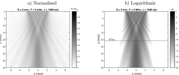
a) Normalised b) Logarithmic D = 5 mm., F = 5 mHz., c = 1500 m/s. -6 -4 -2 0 2 4 6 x (mm) 0 5 10 15 20 25 30 35 40 z (mm) 0 0.1 0.2 0.3 0.4 0.5 0.6 0.7 0.8 0.9 1 P/ρcU₀ D = 5 mm., F = 5 MHz., c = 1500 m/s D2_/4λ -6 -4 -2 0 2 4 6 x (mm) 0 5 10 15 20 25 30 35 40 z (mm) -20 -18 -16 -14 -12 -10 -8 -6 -4 -2 0 db

Figure 3.5: Numerical model of 2D pressure distribution

to the two dimensional model which considers the source to be a continuous line cylin-der pulsating radially to generate cylindrical waves (see for example Kinsler et al. [30] or Schmerr [32]). Note that as this is a line source, as illustrated in figure 3.3.b, the approx-imation is representative of the two dimensional pressure field across the diameter of a circular element or across the length of a rectangular element. In the far field the pressure response of the single element is

[32]:-p(x, ω) =ρvu0(ω) r 2 πj(kb) | {z } Ap D(θ) z }| { sin(kbsinθ)) kbsinθ ejkr0 √ kr0 | {z } H(r) (3.9)

where the term Ap corresponds to the pressure field of a point source and H(r) is the

superposition of cylindrical wave terms over the entire length of the element. The term

D(θ) is a directivity function representing an angle-dependent scaling of the wave field amplitude. It has the form of the sinc

function:-sin(x)

x (3.10)

and is highly dependent on the wave number,k, and b(where bis the element length/2). Example polar plots of the directivity function for different length elements are presented in figure 3.6. For the instance where the element length,D, isλ/10, the sound pressure is almost uniform in all directions (-90◦ ≤ θ ≤90◦). When D = λthere is some change in

(43)

directivity but the pressure field remains broad. AtD= 4λthe directivity is in a range of

±10◦ but a number of small side lobes are now apparent. Finally with D set to 16.6λ the pattern is similar to that of figure 3.5.b which has a similar geometry and wave number. As discussed in section 2.14 the beam spread is measured in terms of the angle at which the pressure drops by -6 dB from the value along the axis (atθ= 0). For the sinc function (sin(x)/x) this value occurs at x = 1.895,

therefore:-θ−6dB =sin−10.6

λ

D (3.11)

The directivity of an ultrasonic element has an important role in the transducer’s sound field. For the last three examples in figure 3.6 the respective -6dB angles for the main lobes are approximately 37◦, 9◦, and 2◦. In practice the elements of most single element ultrasonic transducers are typically tens of wavelengths in diameter and the sound beams are well collimated with most of the sound propagating normal to the transducer’s surface. In contrast a phased array contains a number of relatively small elements and the far field directivity of single elements can vary considerably. However the transducer’s overall di-rectivity becomes a function of the number of elements used and the focal law, as discussed in the next section.

3.7 Phased arrays

An ultrasonic phased array is an arrangement of many identical piezo elements in a straight line pattern. In contrast to the introductory single element circular probe the elements of a phased array are rectangular, as illustrated in figure 3.7.

Cost is the main constraint limiting the number of elements. Not only are the probes themselves expensive but the requirement to provide each element with an individual pulse-receiver, electronic timing and physical wiring adds to the expense and complexity. The simplest method of operation is to use each element in pulse echo mode. Firing a single element, a group of adjacent elements or all elements synthesises a variable width

aperture. Alternatively elements can be fired in sequence to capture a B-scan image.

Although each of these methods is likely to find some application in practice they do not take full advantage of the versatility of the phased array which lies in its ability to steer and focus the beam on both reception and emission. Cohran [33] and Olympus [34] overview various scanning methods for phased arrays. The following section introduces the basic

(44)

a) D = 0.1*λ b) D = 1*λ 0.2 0.4 0.6 0.8 1 30 210 60 240 90 270 120 300 150 330 180 0 0.2 0.4 0.6 0.8 1 30 210 60 240 90 270 120 300 150 330 180 0 c) D = 4*λ d) D = 16.6*λ 0.2 0.4 0.6 0.8 1 30 210 60 240 90 270 120 300 150 330 180 0 0.2 0.4 0.6 0.8 1 30 210 60 240 90 270 120 300 150 330 180 0

Figure 3.6: Normalised pressure at constant distance forλ= 0.3 mm

element 1 width (w)

gap (g) pitch (p) height (h)

element N

(45)

principle before developing the mathematics of beam forming and presenting simulation results.

3.8 Beam steering and focusing

p 1 Focal Point xc= 0 zf xf A g w 2 N lN l2 l1 θs ls

Figure 3.8: Wave paths to a focal point

Figure 3.8 illustrates the geometric paths from the centre of each element to a selected focal point. For an array with pitch p, the distance from the centre of element 1 to the centre of elementi

is:-x1(i) = (i−1)∗pitch (3.12)

Subsequently the position of each element with respect to the centre of the array where

x= 0 is now determined by subtracting an offset, equivalent to half the distance between the centres of two outer

elements:-x(i) =x1(i)−((N−1)∗pitch)/2 (3.13)

Using the centre of the array, xc = 0 and z = 0, as the reference the focal point can be

expressed in cartesian, xf, zf or polar, ls∠θs co-ordinates. The horizontal offset xif from

each element to the focal point

is:-xif(i) =xf −x(i) (3.14)

and the distancel(i) between elementiand the focal point

is:-l(i) =

q

Weld Defect Detection using Ultrasonic Phased Arrays