Credit Risk Evaluation using SVM
Bachelor’s Thesis submitted
to
Prof. Dr. Wolfgang K. H¨ardle
Humboldt-Universit¨at zu Berlin School of Business and Economics Ladislaus von Bortkiewicz Chair of Statistics
by
Han Fu
(551280)
in partial fulfillment of the requirements for the degree of
Bachelor of Science
Acknowledgement
I would like to thank my supervisor Prof. Dr. Wolfgang Karl H¨ardle. for his constructive guidance and suggestions to my thesis. I appreciate that Prof. H¨ardle always replies my E-mails immediately and his time and effort spent on the supervision.
In addition I appreciate Niels Wesselh¨offt, to help me with programming. Also I am grateful to Shi Chen who kindly wrote the note of the presentation for me. Besides thanks to Mr. Leslie Udvarhelyi, he gave me so much help in my thesis registration.
Abstract
A credit risk is the risk of default on a debt that could occur when a debtor could not mange to make required payments. This is a big issue because credit risk is one of the primary risks of the financial institutes. Whether the borrower can pay back the debt and how the banks estimate the debt-paying ability of borrowers is of the interest of this empirical research.
In this paper, in order to predict the company bankruptcy the statistical learning algo-rithms are used. More specifically the discriminant analysis (DA) and support vector machine (SVM) will be employed in the simulation since they are widely applied to classification and regression. Moreover discriminant analysis estimation is utilized as the benchmark model. Thus this paper gives an empirical comparison of predictions of debt-paying ability based on these two methods. Lastly the statistical data is processed with the help of R, an advanced and user-friendly statistical language.
Contents
List of Figures iv
List of Tables v
1 Introduction 1
2 Methods 2
2.1 Definition of Machine Learning . . . 2
2.1.1 Supervised Learning and Unsupervised Learning . . . 2
2.2 Model building . . . 3
2.3 Z-score . . . 3
2.4 Support Vector Machine . . . 5
2.4.1 Margin . . . 5 2.4.2 Optimization problem . . . 8 2.4.3 Lagrange multipliers . . . 9 2.4.4 Kernels . . . 11 3 Data 13 3.1 Data Pre-processing . . . 13 3.1.1 Data Cleaning . . . 13 3.1.2 Feature selection . . . 14 3.2 Split Dataset . . . 16 3.3 R Application . . . 16 4 Results 17 4.1 Results of DA Model . . . 17
4.2 Construction of SVM and Parameters Tunning . . . 18
4.2.1 SVM with kernel ”sigmoid” . . . 19
4.2.2 SVM with kernel ”radial” . . . 19
5 Conclusions 19
List of Figures
1 Illustrating the Machine Learning Task . . . 3
2 Example of logistic regression . . . 5
3 linearly separable data set . . . 6
4 Geommetric margin of an example, ω denotes normal vector . . . 6
5 Support Vector Machine . . . 7
6 Data is mapped to high dimensional feature space . . . 11
7 Confusion Matrix . . . 17
8 Result of grid search with gamma= C= 2∧(−1 : 3) . . . 27
9 Result of grid search with gamma= 2∧(−1 : 3) and C= 2∧(4 : 8) . . . 27
10 ROC and AUC of DA model . . . 28
11 ROC and AUC of SVM with ”sigmoid” . . . 28
List of Tables
1 Summary Statistics. Quantile is abbreviated to ”Qu.” . . . 23
2 First step of variable selection . . . 24
3 Result of variable selection . . . 24
4 Relief feature selection,? denotes a variable that was selected . . . 25
5 Prediction of DA model . . . 25
6 Summary of grid search with C=512 . . . 26
7 SVM with kernel ”sigmoid” after parameters tuning . . . 26
8 SVM with kernel ”radial” using first parameter tuning results. . . 26
9 SVM with kernel ”radial” using 3rd parameter tuning results. . . 26
1
Introduction
Now days Machine Learning is one of the most popular statistical techniques. It has made significant inroads in Data Mining: for example, with the booming FinTech industry, increas-ingly many IT companies are stepping into financial branch. By applying Big Data, Artificial intelligence and Blockchain etc. to traditional financial business, the service is improved and the scope of customer is enlarged.
For instance, the Machine Learning technologies can improve the efficiency of crediting: from the perspective of banks, the major obstacle of crediting is the asymmetric information between banks and borrowers, it is difficult to reach the whole market by the traditional crediting, because such manual methods are too slow and too imprecise to deal with the increasingly sophisticated credit applications. Machine Learning technologies make use of the information on the financial statements to mine more knowledge of the debt-paying abilities of the firms, which is beyond the capability of manual crediting.
The reason why to choose financial statements as the major data resource to judge the credibility of a firm is that, they reveal the most reliable and up-to-date information of a company. Whether a company has credit risk, its financial statements may provide an indication. Considering the identical data resource the Machine Learning can perform better than human is because of its ability of data processing.
In essence the debt-paying ability problem could be regarded as a classifications problem: Companies need to be separated into two groups, either solvent or insolvent. The data which contains the financial condition of a company and the solvent labels is fed to the machine, the machine will learn from the data to generate a relationship between features and labels that automatically suggests whether to accept or reject an credit application. The magic behind the machine is basically the Machine Learning Algorithms. In this paper two methods are used: Discriminant Analysis and Support Vector Machine respectively.
Discriminant analysis (DA), a model belongs to the class of Generalised Linear Models (GLM) which is used in many financial institutions in corporate bankruptcy. The theory is put forward by Altman in 1968, it computes a score (overall index) of company by quoting financial data. The score is fixed on the basis of the statistical financial figures which is used as the core element to assess whether a company will be successful or failing.
In most cases, data can not be linearly separated. SVM (Support Vector Machine) is a relatively new way to deal with nonlinear classifications. Vanpnik has developed the theory for statistical learning theory and used it in optical character recognition (Cortes and
Vap-nik, 1995). SVM is such a method in machine learning that technically is actually a linear classifiers in feature space with the largest margin. Though looking for the largest geometric margin SVM finally transforms the problem as a convex optimization problem.The solutions to this problem is mapping data to high dimensional space. It is possible to map the data into a higher dimensional feature space with kernel function. In application of support vector machine a kernel function is used to simplify the procedure of mapping into high dimensional space. It is to note that the choice of specific functions depends on concrete issue when apply-ing a support vector machine’s kernel. In conclusion comparapply-ing with classical classifications methods SVM is more appropriate in solving the problem of nonlinear classification.
The above methods are employed to the given dataset so as to predict the ability of debt-paying. Before implementing the algorithm the dataset is pre-processed and pretty much work in feature engineering is completed. In order to estimate the performance of two models and different kernels in the identical SVM algorithm, confusion matrix and receiver operating characteristic curve are employed such that the determination of the effectiveness of all models is achieved. Thanks to the confusion matrix a visualized performance of all models is given to help with the interpretation of the results.
2
Methods
2.1 Definition of Machine Learning
In this section a brief review of Machine Learning is given. Arthur Samuel explained the machine learning as that, it’s a field of study that the ability to learn without explicitly programmed (Samuel, 1959). Tom Mitchell gave a more formal definition in 1988: A com-puter program is said to learn from experience E with respect to some class of tasks T and performance measure P if its performance at tasks in T, as measured by P, improves with experience E (Mitchell, 2006).
2.1.1 Supervised Learning and Unsupervised Learning
Machine Learning tasks are classified as supervised learning and unsupervised learning (Muller et al., 2001). For example, classification is a common application of machine learning. Ex-perience data has features and labels. Learning algorithm, more generally, find the relation between features and labels from experience data. When we a new data is given, which only has features without label, we can predict the label through algorithm. In this process,
experience data has not only features but also labels. It is called supervised learning. If the experience data has no labels, data can’t be classified. Obviously, it’s unsupervised learning, also can be called clustering. In this research, only supervised learning is applied.
2.2 Model building
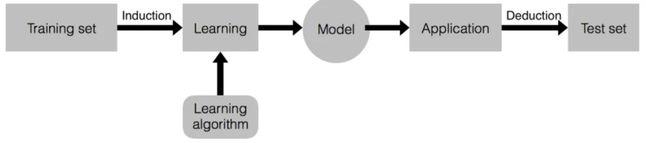
Following machine learning definition, to build a model we should be given experience. Before the created model application, we should measure its performance. Since that, data should splits into two sets (training set and test set). Use training set for model estimation and the other set for model assessment. Figure 1 shows a complete process of Machine Learning tasks.
Figure 1: Illustrating the Machine Learning Task
Finally, if the model is able to predict labels of test set fully meets performance expecta-tion, it can be applied to practice. The new unknown data will be given, and let the model make a prediction.
2.3 Z-score
Multiple discriminant analysis was first used in 1930s. This technique was used to classify an observation into one of several a priori groupings dependent on the observation’s individual characteristics (Altman et al., 2000). Z-score is a famous application of statistical method of discriminant analysis. It was given by Altman in 1968 , that used for predicting bankruptcy. 66 companies’ financial statements were collected by Altman and divided into 2 groups. Each group has 33 samples. DA was good method to classify the binary labels such as bankrupt or non-bankrupt and make predictions. Based on multiple discriminant analysis technique, Altman set a discriminant function as:
V denotes discriminant coefficient, andXmeans independent variable. This form transforms the variables (financial statements) to a scoreZ. Classify the object according computing Z-score. After selection of samples and appropriate statistical technique, independent variables should also be selected. Altman had chosen 5 ratios from a variable list which includes 22 potentially helpful variables.
Z= 1.2X1+ 1.4X2+ 3.3X3+ 0.6X4+ 1.0X5 (2) where X1 = Working Capital / Total Assets, X2 = Retained Earnings / Total Assets, X3 = Earnings Before Interest and Taxes / Total Assets,X4 = Market Value of Equity / Book Value of Total Liabilities and X5 = Sales / Total Assets.
In 1977 Altman had improved his model. Because of the size of bankruptcy companies increasing and the model should correspond with temporal trend. Independent variables were increased to 7, they were changed as(Altman et al., 2000):
• Return On Assets (ROA)
• Stability of earnings
• EBIT/total interest payments
• retained earnings/ total assets
• liquidity
• equity/total capital
• total assets
Compare with the old z-score model, ZETA improvs the predictive accuracy and has more applicability. It could be applied to retail industry firms, not only manufacturers. Both model are linear function, but most economic cases are nonlinear, the linear function reduced the predictive accuracy.
In this paper, we will do the similar thing, based on discriminant analysis method use the linear combination of selected variables for predicting bankruptcy. The variables are selected by stepwise selection (see the Chapter 3.2 Variable Selection), part of the chosen variables may be the same as Altman’s seven variables.
2.4 Support Vector Machine
The basic idea of SVM is distance computation. In this case, x denotes the point, it’s an n -dimensional vector,ydenotes the label. The goal of linear classifiers is to find out a separating hyperplane inn- dimensional space. Separating hyperplane of a classifier with parametersω,
bwith respect to a example is given by this formula:
ω>x+b= 0 (3)
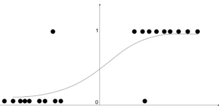
Consider a logistic regression, from figure 2 we know that, on the right side, the probability
y= 1 is higher.
Figure 2: Example of logistic regression
Model it by h(x) = g(v>x). If v>x > 0, the predict equal 1 is more confident. In other words, we would predict ”1” on an input x, if v>x≥0. The larger v>x is, the further from they axis, the larger is P(y = 1). Thus, informally we can think of our predictions as being a very confident thaty=1 ifv>xmuch bigger than 0. Similarly, ifv>xis much smaller than 0, we are very confident that y is equal to zero.
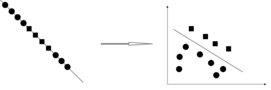
2.4.1 Margin
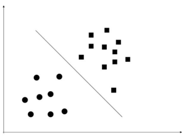
Assuming a binary data set has been divided into training set and test set. We will work with training set first. For example, like the following figure, data lay on the 2-dimensional space, different data were labeled in different shapes. If this data set is linearly separable, there must be a straight line in the middle, which separates data with a greater distance between both sides examples and decision boundary. We use y ∈ {−1,1} inste ad of the common
y ∈ {0,1} notation since it is more convenient in the following formal expressions, and v>x
replaced with ω>x+b. The classification function is written as:
Figure 3: linearly separable data set
Given a training set example (xi, yi). Obviously, if f(x) = 0, x lay on the separating
hyper-plane. Iff(x)>0,yi = 1. Otherwise yi=−1, iff(x)<0.
We define the functional margin of (ω,b) to the training example, ˆ
γi=yi(ω>x+b) (5)
Our prediction is confident in this example ifyi(ω>x+b)>0. We want ω>xi+bas large as
possible for having a large margin. If we replace ω with 2ω and bwith 2b,we can get 2ˆγi. It
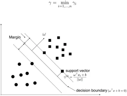
turns out to be very easy to make the functional margin large just by scaling other parameters. But it’s meaningless, we didn’t change the separating hyperplane but only the value off(x). That’s why we need to add a normalization condition to normal vector ω. Consider figure
Figure 4: Geommetric margin of an example,ω denotes normal vector
separating hyperplane. We set ω
||ω|| as unit vector. γ distance between x and x0, algebra
form of a point map to separating hyperplane is written by
x=x0+γ
ω
||ω|| (6)
As the mapped point x0 lay on the separating hyperplane, it must satisfy ω>x0 +b = 0. Hence,
ω>(x−γ ω
||ω||) +b= 0 (7)
Solve this equation forγ, therefore
γ = ω
>x+b
||ω|| (8)
Because of opposite classes’ examples, we write the equation more generally,
γ(i)=y(i)ω >x+b
||ω|| (9)
The distance γ between each data and separating hyperplane is called geometric margin. If the example is correctly classified, this distance will be positive. This is very similar to functional margin except add a normalization condition to ω. Scaling ω will not affect the margin, margin only changes by moving separating hyperplane. Then we need to find a minimal margin of all individual examples, also ideally hope the minimum margin as far as possible from the separating hyperplane.
γ = min
i=1,...,nγi (10)
2.4.2 Optimization problem
In oder to find the maximum geometric margin, we need to solve the following optimization problem:
maxγ,ω,b γ
s.t. y(i)(ω>xi+b)≥γ, iˆ = 1, ..., n ||ω||= 1
(11)
From equation (3) and (6), we know the relation between functional margin and geometric margin:: γ = γˆ
||ω||. Add the condition||ω||= 1 for convenience, the functional margin is equal
geometric margin. y(i)(ω>xi+b)≥γˆ means each sample have the functional margin at least
ˆ
γ. This optimization problem needed to solve are ω and b, so as to maximize the margins. After solving this problem we can derive the optimal margin classifier. Since||ω||= 1, change the problem a little bit, we can get the following problem:
maxγ,ω,b ˆ γ ||ω|| s.t. yi(ω>xi+b)≥γ, iˆ = 1, ..., n (12)
Assume the worst case, let functional margin ˆγ = 1 by scaling ω and b. ˆγ/||ω|| = 1/||ω||, maximize 1/||ω||is equal to minimize ||ω||2. We just add a half there by convention, it make the following work a little nicer. Transform the problem,
minγ,ω,b 1 2||ω|| 2 s.t. yi(ω>xi+b)≥1, i= 1, ..., n (13)
It turns out, the objective function is a quadratic function, and the constraint is linear inequalities. This problem is also called convex quadratic programming. It can be solved either by quadratic programming or Lagrange Duality Theorem. In this situation, compare with quadratic programming, Lagrange Duality Theorem has more efficient. Dual problem is easier solved, and by using dual algorithm the kernel function can be introduced.
For understanding Lagrange Duality Theorem, simply, add a Lagrange multiplier to each constraint, so we can plug the constraint with Lagrange multiplier back to the objective function. L(ω, b, α) = 1 2||ω|| 2− n X i=1 αi[yi(ω>x+b)−1] (14) Set θ(ω) = max αi≥0 L(ω, b, α) (15)
When the constraint is not satisfying, e.g. yi(ω>x+b)<1, thenθ(ω) =inf inity(just setαi= inf). Otherwise, every condition is met, θ(ω) = 1
2||ω||
2 that what we are required minimize.
However, if all the constraints are satisfied, minimize 1 2||ω||
2 is the same as minimize θ(ω) min
ω,b θ(ω) = minω,b maxαi≥0
L(ω, b, α) =p∗ (16)
p∗ is the optimal solution. We will get another equation, after we changing the seat of max
and min max αi≥0 min ω,b L(ω, b, α) =d ∗ (17)
The optimal value d∗ no more equivalent to the initial optimization problem. But we know that,d∗≤p∗, the optimum d∗ of equation (15) suppler a thresholds forp∗. That means, we just need to compute the optimum d∗ of this dual problem of initial problem.
Above is about best linear classifiers. Come back to our work, we need to find the best non-linear classifiers. There exists outlier in other group definitely. Modifying the optimization problem of linear classifier slightly we get non-linear decision boundaries:
minγ,ω,b 1 2||ω|| 2+C n X i=1 ξi s.t. yi(ω>xi+b)≥1−ξi, i= 1, ..., n ξi≥0, i= 1, ..., n (18)
We call ξi slack variable, if ξi ≥ 0, it means i-th example is outliers. When ξi is arbitrary
value, there exists random separating hyperplane satisfy the condition. We have to minimize sum of ξi to subjective function. And it is increased by Cξi. C between the twin goals of
making the||ω||2 large ( which makes the margin small) and of ensuring that most examples have functional margin at least 1 (Ng, 2014).
2.4.3 Lagrange multipliers
Construct the Lagrange function for our optimization problem:
L(ω, b, ξ, α, r) = 1 2||ω|| 2+C n X i=1 ξi− n X i=1 αi[yi(ω>x+b)−1 +ξi]− n X i=1 riξi ∂L ∂ω =ω− n X i=1 αiyixi = 0 ∂L ∂b = n X i=1 αiyi = 0 ∂L ∂ξi =C−αi−ri= 0 (19)
Plugω =Pn i=1αiyixi,Pni=1αiyi = 0 and C=αi+ri back toL. L(ω, b, ξ, α, r) = 1 2||ω|| 2+C n X i=1 ξi− n X i=1 αi[yi(ω>x+b)−1 +ξi]− n X i=1 riξi = 1 2ω >ω+C n X i=1 ξi− n X i=1 αiyiω>x− n X i=1 αiyib+ n X i=1 αi− n X i=1 αiξi− n X i=1 riξi = 1 2ω > n X i=1 αiyixi−ω> n X i=1 αiyixi+ n X i=1 αi+C n X i=1 ξi− n X i=1 αiξi− n X i=1 riξi =−1 2ω > n X i=1 αiyixi+ n X i=1 αi (20) plugω =Pn
i=1αiyixi back twice, and simplify, we get
L(ω, b, ξ, α, r) = n X i=1 αi− 1 2 n X i=j=1 yiyjαiαjx>i xj (21)
Rewrite constraint yi(ω>xi+b) ≥ 1−ξi, i = 1, ..., n as gi(ω) =−yi(ω>xi +b) + 1−ξi ≤
0, i= 1, ..., n.Under KKT conditions1, ∂ ∂ωi L(ω∗, α∗, r∗) = 0, i= 1, ..., n ∂ ∂ri L(ω∗, α∗, r∗) = 0, i= 1, ..., m α∗igi(ω∗) = 0, i= 1, ..., k gi(ω∗)≤0, i= 1, ..., k α∗ ≥0, i= 1, ..., k (22)
only if Lagrange multipliers αi > 0, then g(x)= 0,the examples have functional margin =
1-ξi. We use< xi, xj >instead ofx>i xj to denote inner product.
Put these constraint together, rewritten the equation (21), we can derive the dual problem of the primal Lagrange function as follow:
max α W(α) = n X i=1 αi− 1 2 n X i=j=1 yiyjαiαj < xi, xj > s.t. 0≤αi≤C, i= 1, ..., n n X i=1 αiyi = 0 (23)
1Karush-Kuhn-Tucker Conditions (Gale et al., 1951):
minf(x)
s.t. gi(x)≤0, i= 1, ..., m
Our approach to finding to deriving the optimal margin classifier or SVM will be that, solving along this dual optimization problem for the parameterα∗. The dual optimization problem can be solved. Once we solveα, it can be used for derivingω ( ω=Pn
i=1αiyixi). Moreover,
when we solveαandω, it’s easy to derive b. ω decides the separating hyperplane’s direction. Since we know the orientation of the hyperplane, we just need to decide, where to place the hyperplane. The solution of b,
b=−1
2(xi+xj)
>ω (24)
The intuition of this formula is that, find the worst examples of opposite classes. xi and xj denote different support vectors in different classes. Both of them lay on the margin
boundary(Cizek et al., 2005). It will tell us where to set the threshold and for where to place the separating hyperplane.
2.4.4 Kernels
Now, we have the α, ω, b, and we know the separating hyperplane’s place of this training set. We should test it, and assess its performance. Given a new x, and we should get a value of hypothesis on the value of x. hω,b(x) = g(ω>x+b), ω>x +b can be expressed
as a sum of the inner products between training example and this new value algorithm,
hω,b(x) =g(Pni=1αiyi < xi, x >+b). There exists a representation that allow us to compute
inner products efficiently without representingxi. One replaces inner product< xi, x >with < φ(xi), φ(x)>, where φ denotes the transformation from original dimension data space to
high dimensional set of features.
Consider the figure at below, data was not linearly separable in one-dimensional data space. Mapping it to high dimensional space makes it linearly separable. Once we have the
Figure 6: Data is mapped to high dimensional feature space
dimen-sionality may be high or goes to infinity. Thus sometimes computingφ(x) is computationally very expensive or might be impossible when there is an infinite dimensional vector. Nonethe-less, there exists another approach to compute the inner product between these two vectors easily, that’s called Kernel function.
Assume we have two vectors,x1= (a1, a2),x2 = (b1, b2), after mapping to a high dimen-sion space ,
< φ(x1), φ(x2)>=a1b1+a21b12+a2b2+a22b22+a1a2b1b2 (25) by the way, we find that:
(< x1, x2 >+1)2= 2a1b1+a21b21+ 2a2b2+a22b22+ 2a1a2b1b2+ 1 (26) Equation(25) and equation (26) are similar, we just need to scale the equation and add a constant dimension space. Actually, the equation (26) is equal to the result of transformation of equation(27). φ(X1, X2) = ( √ 2X1, X12, √ 2X2, X22, √ 2X1X2,1) (27)
It means (< x1, x2>+1)2=< φ(X1), φ(X2)>. But the difference lying behind is:
1. One is mapped to the high dimensional space, then calculate it based on the formula of inner product.
2. The other one is directly calculated in the original low dimensional space, it is not necessary to write out the post-mapped result.
We define the kernel function, which is the function that calculates the inner product of two feature vectors in the hidden mapped space. For example, in the previous example, the kernel function is
K(x1, x2) = (< x1, x2 >+1)2 (28) The kernel function is able to simplify the calculation of the inner product in mapped space. Luckly, we need to slove Pn
i=1αiyi < xi, x > +b, and α was computed by the dual problem max α W(α) = n X i=1 αi− 1 2 n X i=j=1 yiyjαiαj < xi, xj > s.t. 0≤αi≤C, i= 1, ..., n n X i=1 αiyi = 0
Since that, we avoid to computation in high dimensional space, but get the same result. Thus we can use linear classifier to separate the data that is not linear separable in original space.
Then the support vector machine produces a nonlinear decision boundary. In this entire process, all we ever need to do is to solve the convex optimization problems.
Above is just a simple example of kernel function. Usually , we should chose from common kernel functions. Some examples of kernel functions.
Linear kernel function
K(x, z) =x∗z
sigmoid kernel function
K(x, z) =tanh(ηx∗z+c0) Gaussian kernel function
K(x, z) =exp(−||x−z||
2 2σ2 )
Later, sigmoid kernel and Gaussian kernel function will be applied in model building.
3
Data
In this study, the database is from the Research Data Center of Humboldt-Universit¨at zu Berlin 2. The original database contains a random sample of 1,000 insolvent and 20,000 sol-vent firms in Germany from 1996 to 2008. In this paper, not the entire data is used.
3.1 Data Pre-processing
Data pre-processing means to deal with training set data, such as addition, deletion and transformation (Kuhn and Johnson, 2013). Original data may be inconsistent and have noise, missing values and outliers. These problems could impact on the forecasting performance significantly. Considering the outcomes of ignoring of data pre-processing, it’s necessary to process the data before loading into programme.
3.1.1 Data Cleaning
The reason to clear the database is that it contains too much useless information: a lot of samples only have the indicator (label) but have no any financial statements. Some financial data is full of the value ”0”, it is so difficult to distinguish this ”0” means actual zero or missed data. Such data could not be well used in the model building consequently they are removed. By reducing the size of data and removing the missing values, both the speed of
2
computing and the accuracy of prediction are improved. 3000 of 21,000 samples are chosen after the data cleaning. The final version contains 2407 solvent and 593 bankrupt companies respectively.
3.1.2 Feature selection
Feature selection affects the model performance directly, hence it is a critical section in data pre-processing and in model building. In most of the cases, combinations of variables could have more effects on forecasting, classification or clustering etc. than individual variables. For example, instead of unemployment, the derived unemployment rate is one of the most important KPI in the capital market to measure the trend of the economy development.
In this paper, from the experience of Altman ZETA, some individual values are trans-formed into combinations.
• Adding equity ratio as a new variable into the dataset could better capture the capital structure and long-term liquidity risk. The logic behind is that equity ratio is a good instrument to estimate financial health.
• EBIT/Interest ratio shows the ratio of pre-interest earnings to the charges required on any debt. It is a risk waring indicator, especially it works well in the tough period of a company, it indicates whether a company can pay the interest to avoid the debt-paying risk and whether this company owns borrowing capacity.
• The bank debt has negative influence on the debt-paying ability, this variable is set as negative value.
• Taking log transformation of total assets. By doing so the absolute values are reduced, it is convenient to do the computation. Log transformation will not change the data character but compress the data size and eliminate the influence of heteroscedasticity.
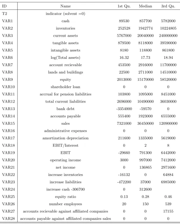
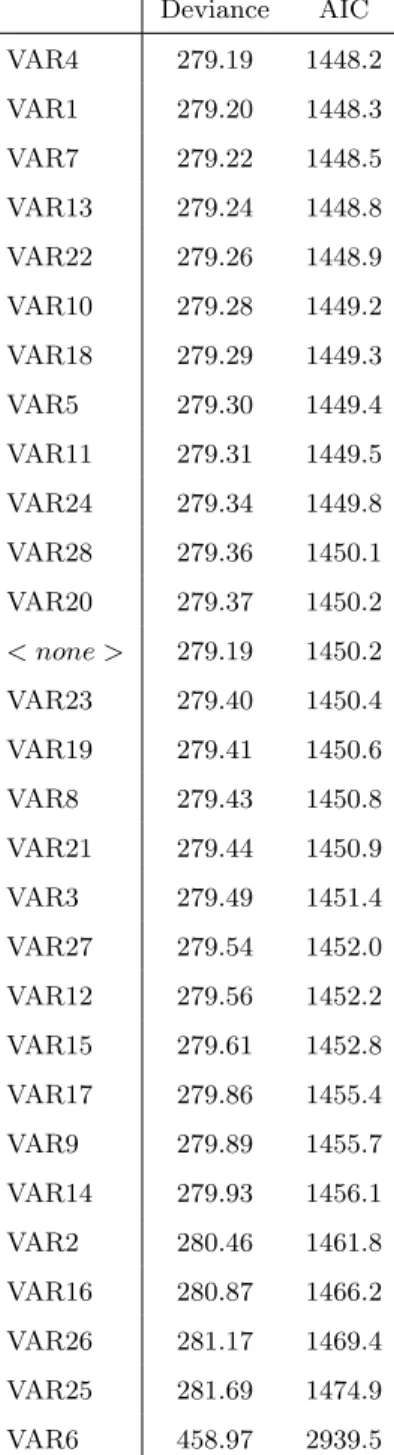
Table 1 presents the summary for each predictor. Followed by feature generation the feature selection process will reduce the noise and improve the predictions of the model by selecting the most relevant variables (H¨ardle and Simar, 2007). In this paper, stepwise selection method is employed for feature selection (H¨ardle et al., 2007) which is based on Akaike information criterion (AIC) that measures goodness-of-fit for the data.
Where ML denotes the maximum likelihood value,m is the number of the parameters. For the best structure, ML should be the largest and AIC should be smallest (H¨ardle et al., 2008). In order to calculate AIC all the variables are included in the beginning, . Based on the formulation of AIC, the value of AIC of all variables would be computed. Then remove the variable, which has the lowest AIC value. New AIC value replaced with last lowest value. And then the rest variables’ AIC are computed. Programme run step by step, until the AIC can not be smaller. Since the stepwise methods is a way of linear variable selection, it will be only used for discriminant analysis.
We will use another method to select the features for SVM, which is called Relief feature selection. Relief feature selection is a feature weighting algorithm, which is put forward by Kira (Kira and Rendell, 1992). Relief assigns each feature a weight based on a distance between instances, if the weight is smaller than the given the relevance threshold, this feature will be removed. The process to compute weight of feature is as below, (Kira and Rendell, 1992)
The model presets training dataset S, relevance threshold τ, and the size of dataset m. 1. Set feature weight vector W equal to 0
2. for i=1 to m do
pick a sample X from S randomly,
find the closest neighbourhood H of X, which has the same label of X. And also find the nearest sample M, which is in different class to X.
3. for i=1 to p do
updateWi =Wi−(xi−H)2+ (xi−M)2
4. Relevance is the averaged weight vector of the value −(xi−H)2+ (xi−M)2, when the
Relevance is larger thanτ, feature will be selected.
In this process, weight of different types including both nominal and numerical features can be computed. Moreover, Relief is not so complicated but pretty efficient, hence Relief method is widely used in machine learning. In this case it is used to select the Variables for SVM. The range of selected features is set as 15, the features are selected from a ranked weight list.
3.2 Split Dataset
To select the training set, 70% of the observed data is randomly extracted, which is used to learn. To estimate the performance of the model on the test set, remaining 30% are used. In order to reduce the bias of the existing dataset, more data is preferably requested. However too small test set is not enough to test the predictive accuracy. It is suggested to split dataset as homogeneous as possible, otherwise the outcome may be substantially different between training and test sets(Kuhn and Johnson, 2013). Hence setting 60% - 80% of the data to as training set is recommended, so 70% is a reasonable figure.
3.3 R Application
In statistical analysis, R is an important instrument. In this project, R is implemented with package ”MASS”, which contains the linear discriminant analysis function. It classifies multivariate observations in conjunction with linear discriminant analysis, and also project data onto the linear discriminants (Ripley et al., 2013).
Packages ”e1071” will help for SVM model building. The svm() function in ”e1071” provides a rigid interface to libsvm along with visualization and parameter tuning methods. Package ”pROC” is a library of functions that supports ROC and AUC plotting in R-Programming.
4
Results
4.1 Results of DA Model
After data splitting and variables choosing, the model of linear discriminant analysis was build by R. By using package ”MASS”, the goal of prediction of labels of the test data set with linear discriminant analysis can be directly completed.
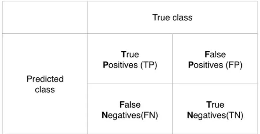
Table 5 shows the forecasting of the test set. Table in this form is called Confusion Matrix. A standard form of Confusion Matrix form is given as figure 7. Confusion Matrix delivers
Figure 7: Confusion Matrix
a clear view of the prediction result. Through comparing the numbers in the matrix, it is clearly to know which model is more accurate.
In the test dataset there are 900 companies. Among them there exist 169 bankrupt companies. Table 5 clearly demonstrates that, the DA model forecasts 158 companies as insolvent, among this prediction, 119 are in reality bankrupt. In other words, the correct prediction percentage is 90.1%.
To visualize the estimation of binary classifier the Receiver Operating Characteristic (ROC) is implemented. ROC in statistics refers to a receiver operating characteristic, or ROC curve, which is a graphical plot that illustrates the performance of a binary classifier system as its discrimination threshold is varied. ROC curve is drawn based on confusion matrix.
X axes is false positive rate (FPR), andY axes is true positive rate (TPR), where
T P R= T P
T P +F N (29)
F P R= F P
F P +T N (30)
Considering the fact that the point (0,1) is on this coordinate, which means FN=0 and TP=1. It is a sign of a perfect classification. By contrast the point (1,0) is the worst classification, because it avoids all of the correct predictions. The model computes the score of each sample being as positive classified. We can get a pair of FPR and TPR by each score, connecting all the points is the ROC curve.
Figure 10 shows the ROC of DA model where FPR and TPR are replaced by sensitivity and specificity. Sensitivity is also called TPR, and specificity is the same as true negative rate (TNR),
T N R= T N
T N+F P (31)
Specificity=1-FPR. The graph with sensitivity and specificity is identical to the one with TPR and FPR, because the range of specificity on the graph is given by [1,0].
AUC is an indicator to measure predictive accuracy. The AUC value is equivalent to the probability that a randomly chosen positive example is ranked higher than a randomly chosen negative example (Fawcett, 2006). As a value, it works as an intuitive presentation of classifier comparison so as to find out the optimal classifier.
4.2 Construction of SVM and Parameters Tunning
The package ”e1071” provides an interface to libsvm with tuning functions. The purpose of tuning functions is to train the model with different parameters so as to improve the overall performance of SVM, in this case the parameters to be tuned are the cost C and gamma (which is also calledξ ). Technically parameters tuning performs a grid search over all available combinations of the two parameters. Since in the beginning the range of gamma andCis unknown, so that an arbitrary range of the two parameters for example gamma=C= 2∧(−1 : 3) is chosen. In this manner the function tune.svm() tunes different combinations ofC and gamma one by one and then returns the best model based on error and dispersion. After the first tuning, the best couple of gamma andC are 4 and 8.
In the figure below, the darker region indicates the better performance of the parameters. Gamma= 4 lies in the middle of ranges which means it is at the optimal value. The next step
is to expand the search range ofC and gamma range remains at 2∧(−1 : 3). More different values of C are tried, and the best value equals to 256. 256 reaches the maximum value of
C in the given range, so in the following steps the larger C is tuned. Eventually the optimal combination of (gamma,C) is (4, 512).
4.2.1 SVM with kernel ”sigmoid”
Plugging the optimal (gamma, C) into the model, SVM with different kernel have different performance on the same data. Surprisingly, the performance of SVM with kernel ”sigmoid” is even worse than the performance of discriminant analysis(90.1%). Although parameters were tuned, the percentage of total correct prediction is only 80.4%. When it comes to the AUC value, the model of SVM scores at only 0.716 while the DA is as high as 0.825. Hence the same conclusion is arrived that DA performs better in this case.
4.2.2 SVM with kernel ”radial”
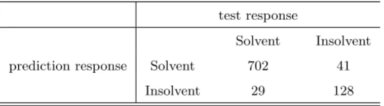
To improve the performance of SVM, another kernel ”radial” is examined in this section. ”radial” is the abbreviation for Gaussian radial basis function kernel. The reason to chose this kernel is because that it is a widely used function especially in classification problem and in general performs very well. Table 8 illustrates that the prediction of SVM with kernel ”radial” has higher accuracy. By using tuning function, the parameters are selected from different tuning process. Comparing these 2 tables, the tuning function improvs the performance apparently. Plugging in the last best parameter into the function, the percentage of total correct prediction reaches at 94.7%. It performs significantly better than the previous models. Besides it proves that the performance of SVM is not only highly dependent on the value of parameters, but also the on the kind of kernels. Plotting ROC and AUC graph of this model, as expected the values of AUC are in the order : AU Cradial > AU CDA > AU Csigmod.
Eventually, the same SVM model is ran but without feature selection, the result is shown by table 10. Comparing this result with table 9, it justifies the feature selection process.
5
Conclusions
Based on the dataset Creditreform the Insolvency is predicted by SVM and DA technique. And then though confusion matrix and value of AUC the predictions performance are tested respectively, the results indicate that the SVM model with Gaussian radial basis kernel per-forms considerably better than others. The final accuracy ratio of prediction can arrive at
94.7% which is a pretty highly acceptable value.
More importantly, it significantly reduces the number of false positive samples, which generally causes the greatest loss of banks. This is because that a false positive case means that, a company receives the credit but finally bankrupt. Comparing with the case of false negative which is a bank rejects a crediting to firm which has the debt-paying ability, the FP case triggers much loss which banks are trying to avoid. Thus SVM apparently reduces the loss possibility of banks.
Honestly speaking, there exist weak points of SVM. For instance the tuning time: tuning parameters runs one by one and the error values are computed by each step is a pretty time-consuming process. Even worse when the range of parameters gets larger, the more time and computer memory will be consumed, which may even breakdown the computer.
In addition to the resource consumption, the prediction accuracy of SVM could be ham-pered by incomplete data. It’s a good way to solve this problem by sharing information among financial institutions and companies, however this triggers the problem of data breach. Hence the insufficient data is one of the restrictions of the applications of SVM.
Moreover, considering the fact that this model uses only the data from a single country in a specific time interval that neglects the differences of financial sectors across time and regions, the generalization of this model to others is reasonably limited.
To the end, as Wolpert said ”No algorithm is generally superior than others. ” (Wolpert and Macready, 1997). This paper takes only DA and SVM into consideration, however to deal with classification issue, in general it is also suggested to use Logistic Regression and Random Forest etc. Consequently, by setting the results of SVM as the benchmark different algorithms in further studies could be implemented.
References
Altman, E. I. et al. (2000): “Predicting financial distress of companies: revisiting the
Z-score and ZETA models,” Stern School of Business, New York University, 9–12.
Cizek, P., W. K. H¨ardle, and R. Weron (2005): Statistical tools for finance and
insur-ance, Springer Science & Business Media.
Cortes, C. and V. Vapnik (1995): “Support-vector networks,” Machine learning, 20,
273–297.
Fawcett, T. (2006): “An introduction to ROC analysis,” Pattern recognition letters, 27,
861–874.
Gale, D., H. W. Kuhn, and A. W. Tucker(1951): “Linear programming and the theory
of games,” Activity analysis of production and allocation, 13, 317–335.
H¨ardle, W., N. Hautsch, and L. Overbeck (2008): Applied quantitative finance,
Springer Science & Business Media.
H¨ardle, W., R. Moro, and D. Sch¨afer(2007): “Estimating probabilities of default with
support vector machines,” .
H¨ardle, W. and L. Simar (2007): Applied multivariate statistical analysis, vol. 22007,
Springer.
Kira, K. and L. A. Rendell(1992): “The feature selection problem: Traditional methods
and a new algorithm,” in AAAI, vol. 2, 129–134.
Kuhn, M. and K. Johnson (2013): Applied predictive modeling, Springer.
Mitchell, T. M. (2006): The discipline of machine learning, vol. 9, Carnegie Mellon
Uni-versity, School of Computer Science, Machine Learning Department.
Muller, K.-R., S. Mika, G. Ratsch, K. Tsuda, and B. Scholkopf (2001): “An
introduction to kernel-based learning algorithms,” IEEE transactions on neural networks, 12, 181–201.
Ng, A. (2014): “Machine Learning,” http://cs229.stanford.edu/notes/cs229-notes3.pdf,
Ripley, B., B. Venables, D. M. Bates, K. Hornik, A. Gebhardt, D. Firth, and
M. B. Ripley (2013): “Package ‘MASS’,” CRAN Repository. http://cran. r-project.
org/web/packages/MASS/MASS. pdf.
Samuel, A. L.(1959): “Some studies in machine learning using the game of checkers,”IBM
Journal of research and development, 3, 210–229.
Wolpert, D. H. and W. G. Macready(1997): “No free lunch theorems for optimization,”
ID Name 1st Qu. Median 3rd Qu.
T2 indicator (solvent =0)
VAR1 cash 89530 857700 5782000
VAR2 inventories 252528 1942774 10224805
VAR3 current assets 5767000 20040000 240000000
VAR4 tangible assets 879500 8118000 39590000
VAR5 intangible assets 8180 118800 861800
VAR6 log(Total assets) 16.32 17.73 18.94
VAR7 account recievable 453500 2916000 11700000
VAR8 lands and buildings 22500 2711000 14510000
VAR9 equity 2013000 15170000 58520000
VAR10 shareholder loan 0 0 0
VAR11 accrual for pension liabilities 103800 1095000 8451000
VAR12 total current liabilities 2696000 10490000 36030000
VAR13 bank debt -3354000 -59570 0
VAR14 accounts payable 555400 1923000 6555000
VAR15 sales 7321000 36450000 120900000
VAR16 administrative expenses 0 0 0
VAR17 amortization depreciation 211600 1335000 5619000
VAR18 EBIT/Interest 0 2 8
VAR19 EBIT -29660 791300 6442000
VAR20 operating income 3000 997000 7412000
VAR21 net income 0 136865 2971600
VAR22 increase inventories -16132 0 64884
VAR23 increase liabilities -472200 37000 6985000
VAR24 increase cash -306700 0 312600
VAR25 equity ratio 0.13 0.28 0.46
VAR26 number employees 20 150 539
VAR27 accounts recievable against affiliated companies 0 0 17155
VAR28 accounts payable against affiliated companies sales 0 0 0
Deviance AIC VAR4 279.19 1448.2 VAR1 279.20 1448.3 VAR7 279.22 1448.5 VAR13 279.24 1448.8 VAR22 279.26 1448.9 VAR10 279.28 1449.2 VAR18 279.29 1449.3 VAR5 279.30 1449.4 VAR11 279.31 1449.5 VAR24 279.34 1449.8 VAR28 279.36 1450.1 VAR20 279.37 1450.2 < none > 279.19 1450.2 VAR23 279.40 1450.4 VAR19 279.41 1450.6 VAR8 279.43 1450.8 VAR21 279.44 1450.9 VAR3 279.49 1451.4 VAR27 279.54 1452.0 VAR12 279.56 1452.2 VAR15 279.61 1452.8 VAR17 279.86 1455.4 VAR9 279.89 1455.7 VAR14 279.93 1456.1 VAR2 280.46 1461.8 VAR16 280.87 1466.2 VAR26 281.17 1469.4 VAR25 281.69 1474.9 VAR6 458.97 2939.5
Table 2: First step of variable selection
Deviance AIC < none > 280.05 1433.4 VAR12 280.27 1433.8 VAR27 280.47 1435.9 VAR21 280.47 1435.9 VAR15 280.73 1438.7 VAR16 280.93 1440.9 VAR8 280.95 1441.0 VAR9 280.97 1441.3 VAR23 281.00 1441.6 VAR2 281.23 1444.0 VAR3 281.62 1448.2 VAR17 281.71 1449.1 VAR26 281.85 1450.6 VAR25 282.56 1458.2 VAR16 283.12 1464.1 VAR6 460.87 2925.9
Var attribute importance status VAR1 -1.022215e-04 ? VAR2 -1.231879e-03 VAR3 -6.412287e-05 ? VAR4 -1.813004e-04 ? VAR5 2.035164e-04 ? VAR6 -1.324257e-04 ? VAR7 -1.667163e-04 ? VAR8 -2.202989e-04 VAR9 -3.211535e-04 VAR10 -1.733980e-04 ? VAR11 -7.173556e-04 VAR12 -3.901673e-04 VAR13 -2.728742e-05 ? VAR14 -1.619685e-04 ? VAR15 -1.214501e-04 ? VAR16 -1.004977e-03 VAR17 -1.672692e-04 ? VAR18 -2.010160e-04 VAR19 -1.880669e-04 ? VAR20 -4.339745e-04 VAR21 -4.895063e-04 VAR22 -1.059422e-03 VAR23 -7.025068e-04 VAR24 -2.394900e-04 VAR25 3.560641e-05 ? VAR26 5.480271e-05 ? VAR27 -5.127143e-04 VAR28 5.364395e-05 ?
Table 4: Relief feature selection,? denotes a variable that was selected
test response
Solvent Insolvent
prediction response Solvent 692 50
Insolvent 39 119
cost gamma error dispersion 512 0.5 0.05666667 0.01409931 512 1.0 0.05571429 0.01650336 512 2.0 0.05619048 0.01502496 512 4.0 0.05380952 0.01230543 512 8.0 0.05952381 0.01082395
Table 6: Summary of grid search with C=512
test response
Solvent Insolvent
prediction response Solvent 627 72
Insolvent 104 97
Table 7: SVM with kernel ”sigmoid” after parameters tuning
test response
Solvent Insolvent
prediction response Solvent 702 41
Insolvent 29 128
Table 8: SVM with kernel ”radial” using first parameter tuning results.
test response
Solvent Insolvent
prediction response Solvent 702 19
Insolvent 29 150
Table 9: SVM with kernel ”radial” using 3rd parameter tuning results.
test response
Solvent Insolvent
prediction response Solvent 694 21
Insolvent 37 148
Figure 8: Result of grid search with gamma= C= 2∧(−1 : 3)
Figure 9: Result of grid search with gamma= 2∧(−1 : 3) and C= 2∧(4 : 8)
Figure 10: ROC and AUC of DA model
Figure 11: ROC and AUC of SVM with ”sigmoid”
Declaration of Authorship
I hereby confirm that I have authored this Bachelor’s thesis independently and without use of others than the indicated sources. All passages which are literally or in general matter taken out of publications or other sources are marked as such.
Berlin, Oct 6, 2016