Simplex basis function based sparse least
squares support vector regression
Article
Accepted Version
Creative Commons: AttributionNoncommercialNo Derivative Works 4.0
Hong, X., Mitchell, R. and Di Fatta, G. (2019) Simplex basis
function based sparse least squares support vector
regression. Neurocomputing, 330. pp. 394402. ISSN 0925
2312 doi: https://doi.org/10.1016/j.neucom.2018.11.025
Available at http://centaur.reading.ac.uk/80789/
It is advisable to refer to the publisher’s version if you intend to cite from the
work. See
Guidance on citing
.
To link to this article DOI: http://dx.doi.org/10.1016/j.neucom.2018.11.025
Publisher: Elsevier
All outputs in CentAUR are protected by Intellectual Property Rights law,
including copyright law. Copyright and IPR is retained by the creators or other
copyright holders. Terms and conditions for use of this material are defined in
the
End User Agreement
.
www.reading.ac.uk/centaur
CentAUR
Simplex Basis Function Based Sparse Least
Squares Support Vector Regression
Xia Hong, Richard Mitchell, Giuseppe Di Fatta
Abstract
In this paper, a novel sparse least squares support vector regression algorithm, referred to as LSSVR-SBF, is introduced which uses a new low rank kernel based on simplex basis function, which has a set of nonlinear parameters. It is shown that the proposed model can be represented as a sparse linear regression model based on simplex basis functions. We propose a fast algorithm for least squares support vector regression solution at the cost ofO(N) by avoiding direct kernel matrix inversion. An iterative estimation algorithm has been proposed to optimize the nonlinear parameters associated with the simplex basis functions with the aim of minimizing model mean square errors using the gradient descent algorithm. The proposed fast least square solution and the gradient descent algorithm are alternatively applied. Finally it is shown that the model has a dual representation as a piecewise linear model with respect to the system input. Numerical experiments are carried out to demonstrate the effectiveness of the proposed approaches.
Index Terms
least squares support vector regression, low rank kernels, simplex basis function.
I. INTRODUCTION
With strong support from its underlying statistical learning theory, the support vector machine (SVM) [2] including the support vector machine for regression (SVR) [3] is a powerful modelling tool able to provide excellent model generalization. Originally the model estimation of SVM corresponds to a quadratic programming optimization problem. The SVM/SVR are regarded as sparse models which also avoid local minima for exceptional modeling performance, however they are computationally demanding. There are significant algorithmic developments such as sequential minimal optimization (SMO) [5] which is aimed at increasing computation speed. In the smooth SVR (SSVR) approach an accurate smooth approximation has been proposed to replace the insensitive loss function in SVR, hence relaxing the optimization problem into an unconstrained one [4], providing a significant speed up. A heuristic method based on a measurement of similarity among samples to reduce data samples for accelerating training was proposed in [6]. A novel geometric framework, based on which new SVR models and algorithms are proposed in [7], these use convex hull algorithms for data reduction. The SVR has also been applied in applications in nonstationary settings, e.g., time-series prediction in nonlinear environment [8], and interval regression analysis
in time-varying environment [9]. A major advance for computational efficiency is the introduction of least squares support vector machine (LSSVM) and least squares support vector regression (LSSVR), which uses equality constraints [10] so that closed form least squares type solutions are available. Note that LSSVM/LSSVR will produce a nonsparse model loosing sparseness property. In common to general kernel methods, LSSVM/LSSVR also have the limitation that the kernel function must be evaluated for all possible pairs of system inputs, potentially infeasible for large scale data modeling problems.
The modelling of real-world data from highly complex, nonlinear structures demands computationally fast kernel methods. Low-rank matrix approximation is an effective tool in alleviating the memory and computational burdens of kernel methods and sampling. For example, the Nystr¨om method has been successfully applied to efficient kernel learning [11]. It randomly samples a subset of training examples and computes a kernel matrix for the random samples. It then represents each data point by a vector based on its kernel similarity to the random samples and the sampled kernel matrix. Alternatively the method of random Fourier features is another popular approach [12], in which the kernel function is approximated by the inner product of a randomized feature map. Note that these low rank kernel approximations will introduce additional generalization errors in the generation performance, which is of theoretic interest [13].
Alternatively, a nonlinear system can be approximated by locally linear systems as piecewise linear systems. Various piecewise linear models exist such as lattice piecewise linear representation [14], hinging hyperplanes (HH) [15] and piecewise affine models [16]. Notably the hinging hyperplane (HH), which uses a hinge function as basis functions, is shown to be a powerful model representation for nonlinear systems since it is endowed with proven approximation capabilities to arbitrary nonlinear functions [15]. Recently a new simplex basis function (SBF) model [20] has been introduced which can be viewed as a HH model and hence has the same approximation capability as HH. Often the use of linear functions to the system input brings the benefit of model interpretability. Moreover there are also rich linear system theory which could be exploited if the model is in the form of linear or piecewise linear form.
In this paper a new low rank kernel based on the simplex basis function has been introduced, based on which a novel sparse least squares support vector machine regression is developed. The proposed model can be represented as a sparse nonlinear SBF model, as well as a piecewise linear model. This framework enables the derivation of a fast algorithm for least squares support vector regression solution at the cost ofO(N). The proposed kernels come with a set of nonlinear parameters, which needs to be adjusted, and it is proposed that the gradient descent algorithm is applied to minimize the mean square errors. Our overall estimation algorithm therefore alternates between the fast LSSVR solution and SBF kernel parameters estimation of the gradient descent algorithm. The advantage of the proposed model is twofold; not only achieve fast LSSVR-SBF estimation, but also to obtain a sparse model which has a dual representation as a piecewise linear model which provides gradient information with ease. Specifically our proposed SBF based low kernels enable us to exploit the structural property of the resultant kernel matrix for fast matrix inversion, which is not valid for conventional Gaussian kernels commonly used in conventional LSSVR models. Similarly since we adopted the recently proposed simplex basis function (SBF) model [20], the model
requires us to devise a new gradient algorithm which is devoted to parameter estimation within the SBF functions. The remainders of this paper are organized as follows. Section II describes preliminaries of the LSSVR model. Section III initially introduces the proposed kernels based on SBF, the LSSVR-SBF model representation a sparse model, and then learning algorithms are introduced including computational complexity analysis and the property of the dual representation of piecewise linear model. Numerical experiments are carried out in Section IV with comparisons with other benchmark approaches in terms of the modeling performance. Section V is devoted to conclusions.
II. LEAST SQUARES SUPPORT VECTOR REGRESSION
Many kernels methods are based on a fixed nonlinear feature mapping in some feature spaceF as
x∈ ℜm→ϕ(x)∈ F, (1)
endowed with aMercer kernel function
k(x(i),x(j)) =ϕ(x(i))Tϕ(x(j)) (2) which is defined as the inner product of two points in the feature spaceFas a symmetric function of its arguments. Suppose a block of training data set denoted asDN, comprisingN input vectorsx(1)...x(N), with corresponding
target values y(1) ... y(N) where y(k) ∈ R. The least square support vector machine for regression problem (LSSVR) [19] is based on a linear model of the form
ˆ
y(x) =wTϕ(x) +b, (3) wherew is vector of parameters. The optimization problem is given by
γ 2 N ∑ n=1 e2(n) +1 2∥w∥ 2, (4)
subject to y(n) = wTϕ(x(n)) +e(n), n = 1, ..., N. Denote e = [e(1), e(2), ..., e(N)]T as the modeling error
vector, and introduce a = [a1, ..., aN]T, where an are Lagrange multipliers for each of the equality constraint,
giving the Lagrangian function
L(w,e;a) =γ 2 N ∑ n=1 e2(n) +1 2∥w∥ 2 − N ∑ n=1 an{wTϕ(x(n)) +e(n)−y(n)},
whereγ >0 is a preset regularization parameter. We now optimize outw, band{e(n)} to give ∂L ∂w =0→ w= ∑N n=1anϕ(x(n)) ∂L ∂b = 0→ ∑N n=1an = 0 ∂L ∂e(n) = 0→ an =γe(n) ∂L ∂an = 0→ wTϕ(x(n)) +b+e(n)−y(n) = 0.
In many kernel methods we do not need to knowϕ(x), but work on a well defined kernel functionk(x,y)using the kernel trick due to (2). After eliminating w, e(n), and using kernel trick, the solution for the dual problem is
b a = 0 1T 1 K+I/γ −1 0 y (5)
where y = [y(1), ..., y(N)]T, and the kernel matrix over the training input data set is a positive semi(definite)
matrix and given as
K= k(x(1),x(1)) · · · k(x(1),x(N)) · · · · · · · · · k(x(N),x(1)) · · · k(x(N),x(N)) ∈ ℜ N×N (6)
I is the identity matrix and1is the vector of all ones with appropriate dimensions. The model prediction is given by ˆ y(x) = N ∑ n=1 ank(x,x(n)) +b. (7)
In spite of the advantage of providing a neat closed form solution, LSSVR has two limitations as would happen in other kernel methods. The computational cost of matrix inversion is in the order ofO(N3), meaning that it does
not scale well with data size N, limiting the training data size to be moderate. Additionally, the LSSVR is not a sparse model since the model size is the same as train sample sizeN, implying that to evaluate a new data point one needs to access all the training data set. In general, one disadvantage associated with most kernel methods is that they do not scale well with large data sets. Hence the low rank kernel approximations are often considered [11, 12] since they allow reduction of computation time toO(N2). In this work we propose a new type of low rank kernel,
that lends itself to new learning algorithms and model representation free of the above two limitations.
III. SPARSE LEAST SQUARES SUPPORT VECTOR REGRESSION BASED ON LOW RANKSBFKERNELS
In the following a new type of low rank kernels is initially introduced for LSSVR which leads to some desirable properties. The proposed kernel has a set of nonlinear parameters and model sizeM, hence in addition to estimating
b anda, our modeling task includes estimation of these extra kernel parameters. Our proposed model estimation algorithm is an iterative and hybrid one with the aim of gaining computational advantage by exploiting the special model functional structure induced by the proposed low rank kernel.
We propose a new type of low rank kernel in the form of k(x,y) = M ∑ j=1 ϕj(x;µj,cj)Tϕj(y;µj,cj), (8)
whereϕj(x;µj,cj)is the simplex basis function (SBF) defined as [20]
ϕj(x;µj,cj) = max ( 0,1− m ∑ i=1 µi,j|xi−ci,j| ) (9) in which cj = [ c1,j c2,j· · ·cm,j ]T
∈ ℜm is known as the center vector of the jth SBF unit which controls the
location ofjth SBF, andµj=
[
µ1,j µ2,j· · ·µm,j
]T
∈ ℜm
+ is the shape parameters vector that control the shape of
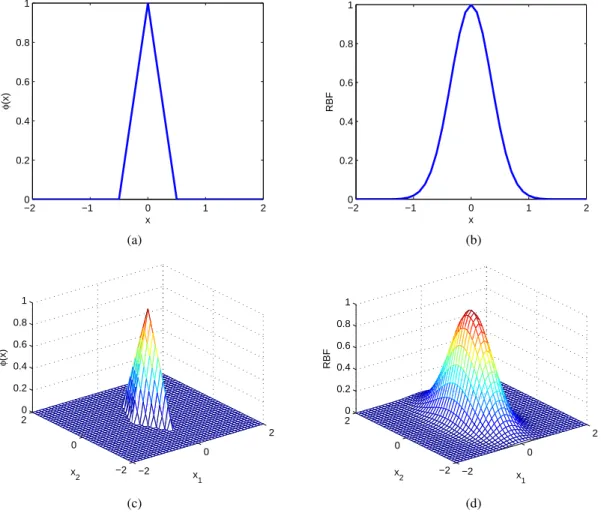
jth SBF. The output of SBF functions is illustrated in Fig. 1. From Fig. 1(a) it is clear that the maximum output is limited as one at the centers, and the responsive region width in one input direction is µ1, inversely proportional to the shaping parameterµ. From Fig. 2(b) it can be seen the SBF output is only nonzeros around the center within a hyper-polygon shaped region. Within this responsive region, it is composed of 2m locally linear models, each
occupying one of2m subregions. The SBF can be visually compared with the well known Gaussian radial basis
function (RBF) via Fig. 1(a) versus its counterpart Fig. 1(b) as well as Fig. 1(c) versus its counterpart Fig. 1(d). Given a collection of dataDN, clearly the associated kernel matrix is given by
K=ΦΦT (10)
withΦ= [ϕ1, ...,ϕM].ϕj= [ϕ(x(1)), ..., ϕ(x(N))]T. Note that (6) can be represented as
ˆ y(x) = N ∑ n=1 an M ∑ j=1 ϕj(x;µj,cj)Tϕj(x(n);µj,cj) +b = M ∑ j=1 θjϕj(x;µj,cj) +b= [ϕ(x)]Tθ+b (11) whereθj= ∑N
n=1anϕj(x(n);µj,cj),θ= [θ1, ..., θM]T, which can be expressed in vector form as
θ=ΦTa. (12)
Equation (12) bridges the original nonsparse LSSVR into a sparse SBF model with onlyM terms, based on M
SBF basis functions. In the proposed algorithm, we will setM as small as possible depending on data sets. From our experience very sparse model can be obtained in comparison with other modeling schemes due to the flexibility of the SBF basis functions.
A. Fast LSSVR parameter estimation
Given that the set of nonlinear parameterscjandµj,Φbecomes fixed, we propose a fast way of calculating (5)
−2 −1 0 1 2 0 0.2 0.4 0.6 0.8 1 φ (x) x −2 −1 0 1 2 0 0.2 0.4 0.6 0.8 1 x RBF (a) (b) −2 0 2 −2 0 2 0 0.2 0.4 0.6 0.8 1 x1 x2 φ (x) −2 0 2 −2 0 2 0 0.2 0.4 0.6 0.8 1 x 1 x 2 RBF (c) (d)
Fig. 1. Graphical illustration of SBF functions centered at origin in comparison with RBF functions; (a) 1D functionϕ(x) = max(0,1− 2|x|);(b) 1D RBF function functionexp(−4x2); (b) 2D functionϕ(x) = max(0,1−2|x
1|−|x2|
)
; (d) 2D RBF functionexp(−4x2 1−x22
)
computational cost of matrix inversion can be reduced to O(M N), enabling fast parameter estimation. Defining ˜ Φ= 0 · · · 0 ϕ1 · · · ϕM ∈ ℜ(N+1)×M (13) (5) becomes b a = 0 1T 1 I/γ +Φ ˜˜ΦT −1 0 y . (14)
Applying the matrix inversion lemma to (14), we obtain b a = ( I− 0 1T 1 I/γ −1 ˜ Φ(I+Φ˜T 0 1T 1 I/γ −1 ˜ Φ)−1Φ˜T ) 0 1T 1 I/γ −1 0 y def = q−PΦ˜(I+Φ˜TPΦ˜)−1Φ˜Tq def = q−PΦ˜(I+Q)−1Φ˜Tq (15) in which P = 0 1T 1 I/γ −1 = 1 N −1/γ 1T 1 γ(NI−11T) , (16) and q= 1 N −1/γ 1T 1 γ(NI−11T) 0 y = 1 N 1Ty γ(Ny−11Ty) (17) and Q=Φ˜TPΦ˜=γΦ˜TΦ˜−N γϕ¯ϕ¯T. (18) in which ϕ¯ = [ ¯ϕ1, ...,ϕ¯M]T, andϕ¯j= N1 ∑N k=1ϕj(k).
The proposed algorithm needs to be initialized with a predetermined model sizeM and an initial design matrix Φ, which is based on preset values ofcj,µj,j= 1, ...M. Clustering algorithms can be used to initialize the centers
cj, which accurately reflects the distribution of the data points. Thek−means [21] clustering algorithm is applied
to obtain initial simplex function centers, which is detailed in Algorithm 1 for completeness. While for shaping parametersµi,j in all simplex functions, it is uniformly initialized as µi,j =µ, where µ >0 is a predetermined
constant, i.e. we presetµj =µ1.
The fast LSSVR algorithm using SBF low rank kernel is summarized in Algorithm 2, of which the computational cost is determined by a series of matrix-vector multiplication with the cost at O(N M), matrix multiplication at
Algorithm 1 The k-means clustering algorithm
Require: x(k),k= 1,· · ·, N, and a preset number of centers M.
Ensure: cj,j= 1,· · ·, M, that yields the minimum ofJ =
∑M
j=1 ∑
x(k)∈Sj∥x(k)−cj∥ 2 1: Randomly selectM data points fromDN as initial centerscoldj .
2: Randomly draw a data point x(k)fromDN.
3: From allcoldj ,j= 1,· · ·, M, find the nearest center tox(k), denoted ascoldi .
4: Update cnew
i =coldi +ϵ(x(k)−coldi ), where ϵ >0is the predetermined learning rate.
5: Set cnew
i as coldi .
6: Goto Step 2 until a sufficient large number of iterations, or convergence has been reached.
7: Returncnew
j as cj,i= 1,· · ·, M.
Algorithm 2 Summary of fast LSSVR algorithm using SBF low rank kernel.
Require: Φ,y.
Ensure: Ensurebanda are found for givenΦ.
1: Construct Φ˜.
2: Calculate b,a using (15)-(18).
3: Returnb,a.
B. Iterative estimation of SBF kernels using proposed gradient descent algorithm
Given a training data set DN, consider parameter estimation for the proposed kernel which is specified by a
set of nonlinear parameters cj andµj (j = 1, ...M). We propose an iterative approach by adjusting cj,µj, ∀j,
associated withϕj(x)using a new gradient descent algorithm, while {a,b} are fixed. Our optimization criterion
is based on minimizing the sum of squares of errors (SSE), given by
J(j)(cj,µj) = N ∑ n=1 e2(x(k)) =eT(y−Ka−b1). (19) We have ∂J(j) ∂µi,j =−e T ∂K ∂µi,ja i= 1, ..., m ∂J(j) ∂ci,j =−e T∂K ∂ci,ja i= 1, ..., m (20) in which ∂K ∂µi,j = ( ∂ ∂µi,j ϕj)ϕTj +ϕj( ∂ ∂µi,j ϕj)T ∂K ∂ci,j = ( ∂ ∂ci,j ϕj)ϕ T j +ϕj( ∂ ∂ci,j ϕj)T (21) where ∂ ∂µi,j ϕj = [ ∂ϕj(x(1)) ∂µi,j , ...,∂ϕj(x(N)) ∂µi,j ]T ∂ ∂ci,j ϕj= [∂ϕj(x(1)) ∂ci,j , ...,∂ϕj(x(N)) ∂ci,j ]T (22)
Algorithm 3 The proposed LSSVR Algorithm with SBF Kernels.
Require: DataDN. Model sizeM. Regularization parameterγ. Initial shaping parameterµ. Iteration numberIter.
Ensure: Parameters (cj,µj,j= 1, ...M),b,aare obtained.
1: Apply Algorithm 1 (thek−means clustering algorithm) to initializecj,j= 1, ...M. Set allµi,j asµ.
2: forl= 1, ..., Iter do
3: Form Φfrom DN based oncj,µj,j = 1, ...M.
4: Apply Algorithm 2 to findb,a.
5: forl= 1, ..., M do
6: Adjustcj,µj using (20)-(27).
7: end for
8: Apply Algorithm 2 to updateb,a.
9: end for
10: Returncj,µj,j= 1, ...M,b anda.
which are calculated by
∂ϕj(x(k))
∂µi,j
=−|xi(k)−ci,j|Id(k), i= 1, ..., m (23)
∂ϕj(x(k))
∂ci,j
=µi,jsign(xi(k)−ci,j)Id(k), i= 1, ..., m (24)
in which Id(k)is an indication function given as
Id(k) = 1 if ∑mi=1µi,j|xi(k)−ci,j|<1 0 otherwise (25) and sign(s) = 1 s >0 0 s= 0 −1 s <0 . (26)
Finally by taking into account the positive constraints for the shaping parameters µj, we propose the constrained normalized gradient descent algorithm, as expressed as
ci,j = ci,j−η· ∂J (j) ∂ci,j/∥ ∂J(j) ∂cj ∥ ˜ µi,j = µi,j−η·∂J (j) ∂µi,j/∥ ∂J(j) ∂cj ∥ µi,j = max ( 0,µ˜i,j ) (27)
for i= 1, ...m, where η >0 is a preset smaller learning rate.
To update all SBF kernel, Equations (20)-(27) are simply applied to M SBF units (j= 1, ..., M) in turn while fixingb,a, and all other SBF units. The computational cost is thereforeO(M2N). Note that this low computation
cost is based on the fact that (21) has low rank, and in calculating the gradient vector (20), (21) can be in its split form, which are premultiplied witheT,aTrespectively.
C. Summary of the LSSVR-SBF algorithm
The proposed algorithm is summarized in Algorithm 3. It starts with k-means clustering algorithm for initialization of SBF centers with a cost at O(N), then the fast least squares LSSVR solution in Section III-A and gradient decent algorithm in Section III-B are alternatively applied for a predetermined number of iterations. The overall computational complexity is dominated by the gradient descent algorithm with O(M2N). Hence our proposed
algorithm has a linear complexity ofO(N), scaled further by model sizeM, number of intermediate variables and iteration number. Thanks to the special structure of the proposed low rank kernels, which enables fast least squares solution as proposed, this further allows the kernels to be trained using the gradient descent algorithm iteratively. Furthermore we can often obtain a very sparse model due to the use of the flexible SBF kernels which are learnt from data automatically, with very little presetting parameters. The overall algorithm is based on the alternative application of the LSSVR and gradient descent algorithms which have known convergence. LSSVR is a global optimal algorithm which finds the optimal b, a. The gradient descent algorithm depends on the learning rate η
which should be set as sufficiently small so that the MSE is decreasing per iteration for general smooth function. Since the SBF model is not based on a smooth function, the MSE per time step may still be slightly increasing even for very small learning rates, so that the MSE is in general decreasing but not smooth.
D. Piecewise linear model dual representation
In the following, a special property is analyzed, which is referred to as the dual representation of SBF as a piecewise linear model (Lemma 1).
Lemma 1: The SBF modelyˆ(x)can be represented as a piecewise locally linear model with respect to inputx as
ˆ
y(x) =α(x)Tx+β(x) +b, (28) whereα(x)andβ(x)are piecewise constants, with the properties
(i) ∂ ∂xα(x) =0, ∂ ∂xβ(x) = 0, (29) (ii) ∂ ∂xf(x) =α(x). (30)
Proof:Consider any given input vectorx, (5) can alternatively be represented as
ˆ y(x) = ∑ j∈S(x) θj ( 1− m ∑ i=1 µi,j|xi−ci,j| ) , (31)
whereS(x)∈[1, ..., M]is the index set of j, satisfying condition∑im=1µi,j|xi−ci,j|<1. We have ˆ y(x) = ∑ j∈S(x) θj− ∑ j∈S(x) θj m ∑ i=1 µi,j|xi−ci,j|+b = m ∑ i=1 xi ∑ j∈S(x) θjµi,jsign ( ci,j−xi ) + ∑ j∈S(x) θj ( 1− m ∑ i=1
µi,jci,jsign
( ci,j−xi )) +b =α(x)Tx+β(x) (32) andα(x) = [α1(x), ..., αm(x)]T, in which αi(x) = ∑ j∈S(x) θjµi,jsign ( ci,j−xi ) , i= 1, ..., m β(x) = ∑ j∈S(x) θj ( 1− m ∑ i=1
µi,jci,jsign
( ci,j−xi )) +b (33) So that we have ∂x∂ iαi(x) = 0, ∂ ∂xiβ(x) = 0.Hence ∂ ∂xyˆ(x) =α(x). (34) This concludes the proof.
Clearly SBF’s dual representation as a piecewise linear model with respect to input vectorxis useful for extracting gradient information from an identified model in the similar way as a linear model, except that these are locally dependent. Moreover, since there are abundant theories in linear systems, e.g. in linear control systems/signal processing, this piecewise linear model representation can be further exploited for its usefulness depending on applications, which are our current/future work. For example, the proposed model can be extended to a generalized predictive controller where the gradient information are needed for calculating the optimal control signals [22], in which the least square support regression model has been successfully applied. Further works will appear as separate publications.
IV. SIMULATIONSTUDY
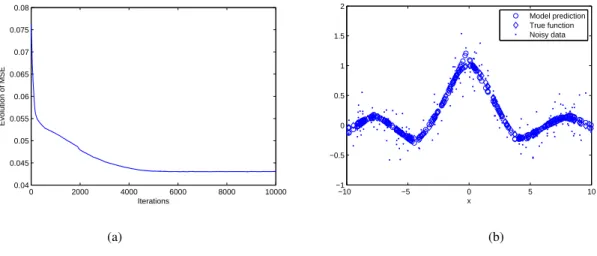
Example 1 (Nonlinear static function approximation): Consider using LSSVR-SBF to approximate an unknown scalar function
f(x) =sin(x)
x . (35)
A data set of two hundred points was generated fromy=f(x) +ξ, where the inputxwas uniformly distributed in [-10,10] and the noiseξ was Gaussian with zero mean and standard deviation 0.2. The data were very noisy. The proposed LSSVR-SBF algorithm was applied with model sizeM = 3,µ= 0.2,Iter= 10000, γ= 500, and the learning rateη= 0.001. The modeling results are plotted in Fig. 2 (a) and (b), respectively. Fig. 2 (b) demonstrates
that the model can approximate the true underlying function well. In fact the modeling MSE with respective to the true function converges to 0.0022.
0 2000 4000 6000 8000 10000 0.04 0.045 0.05 0.055 0.06 0.065 0.07 0.075 0.08 Iterations Evolution of MSE −10 −5 0 5 10 −1 −0.5 0 0.5 1 1.5 2 x Model prediction True function Noisy data (a) (b)
Fig. 2. Results of Example 1: (a)The evolution of mean square error (MSE) and (b) Noisy data, true function and model predictions of a three term model. 0 50 100 150 200 250 300 350 400 3.5 4 4.5 5 5.5 6 Sample System input 0 50 100 150 200 250 300 350 400 2.5 3 3.5 4 4.5 5 Sample System output (a) (b)
Fig. 3. Engine Data: (a) the system inputu(k)and (b) the system outputy(k)
Example 2 (Nonlinear dynamical system): This Engine data set [23] contains 410 data samples of the fuel rack position (the input u(k)) and the engine speed (the output y(k)), collected from a Leyland TL11 turbocharged, direct injection diesel engine which was operated at a low engine speed. The 410 input and output data points of the engine data set are plotted in Fig. 3 (a) and (b), respectively. The first 210data samples were used in training and the last 200 data samples for model testing. The previous study has shown that the data set can be modeled adequately using the system input vector x(k) = [y(k−1) u(k−1) u(k−2)]T, and the best Gaussian RBF
model was provided by thel2-norm local regularization assisted OLS (LROLS) algorithm based on the LOOMSE
also experimented based on the Gaussian kernel with a common varianceτ2. For theε-SVM, the Matlab function
quadprog.mwas used with the algorithm option set as ‘interior-point-convex’. The tuning parameters in theε-SVM algorithm, such as soft margin parameterC [25], were set empirically so that the best possible result was obtained after several trials. For the LASSO, the Matlab function lasso.m was used with 10-fold CV being used to select the associated regularization parameter. For both the ε-SVM and LASSO, we list the results obtained for a range of kernel widthτ values in Table II, for comparison. The proposed LSSVR-SBF algorithm was applied, with the parsimonious principle in mind, by setting the desired model size M as small as possible. For all model sizes, the experimental setting parameters are uniformly set as µ= 0.2, Iter= 2000,γ = 1000, and the learning rate
η= 0.002. The results obtained for a range of model sizeM are listed in Table I. It can be seen that the proposed approach is capable of producing the excellent predictive performance for this benchmark example, even when the model size is only ten.
TABLE I
COMPARISON OF THE MODELING PERFORMANCE FORENGINEDATA.
Algorithm MSE MSE Model
training set test set size LROLS-LOO [24] 0.000453 0.000490 22 ε-SVM (τ = 3) 0.000502 0.000482 208 ε-SVM (τ = 2.5) 0.000480 0.000475 208 ε-SVM (τ = 2) 0.000461 0.000486 208 ε-SVM (τ = 1.5) 0.000415 0.000579 208 ε-SVM (τ = 1) 0.000370 0.000794 208 LASSO (τ= 1.5) 0.000923 0.001010 70 LASSO (τ= 1) 0.000708 0.000748 44 LASSO (τ= 0.5) 0.000706 0.000842 54 LASSO (τ= 0.2) 0.000565 0.000800 81 LASSO (τ= 0.1) 0.000644 0.001907 76 Proposed LSSVR-SBF 0.000473 0.000487 10 Proposed LSSVR-SBF 0.000440 0.000477 15 Proposed LSSVR-SBF 0.000437 0.000464 20
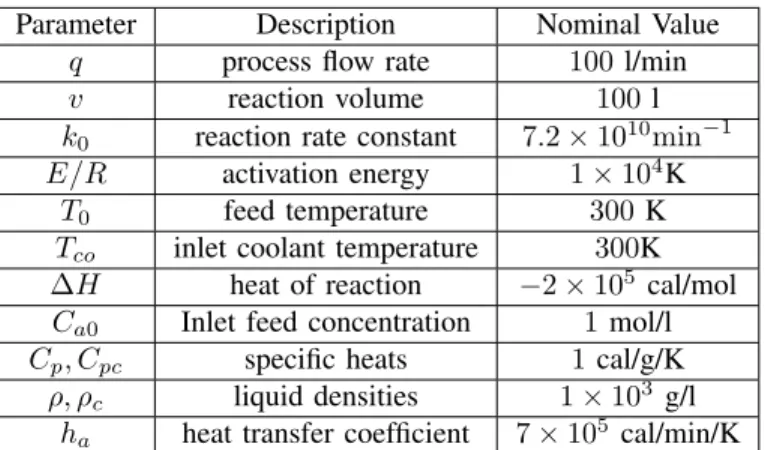
Example 3 (Nonlinear dynamical system): The continuous-stirred tank reactor (CSTR) plant is very common in chemical and petrochemical plants. It has an irreversible, exothermic reaction that occurs in a constant volume reactor and is cooled by a single coolant stream [26]. Within the CSTR two chemicals are mixed and react to produce a product compound A at a concentration Ca(t), with the temperature of the mixture being T(t). The
system output concentrationCa(t)is controlled by regulating the coolant flow rateqc(t)(system input). The CSTR
can be simulated by the following continuous-time, nonlinear, simultaneous, differential equations:
d dtCa(t) = q v ( Ca0−Ca(t) ) −k0Ca(t)e− E RT(t) (36) d dtT(t) = q v ( T0−T(t) ) +k1Ca(t)e− E RT(t) +k2qc(t) ( 1−e− k3 qc(t)(Tc0−T(t))) (37)
where k1 =−∆Hk0/ρCp, k2 = ρcCpc/ρCpv, k3 = ha/ρcCpc, in which CSTR parameters are given in Table
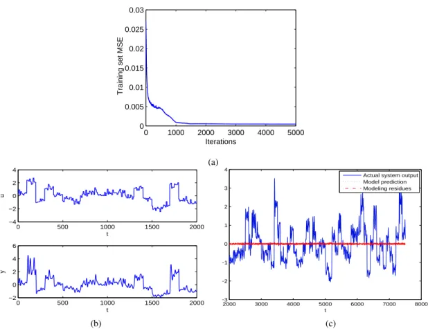
II. For nonlinear system identification of the CSTR, the system input are designed as persistent exciting signal, and we obtain the data set containing 7500 input and output data points from [27]. We build the model based on the normalized data set, with standard deviation for both input and output data as one. Then the output is added a zero mean Gaussian noise with variance of 4×10⁻⁴. 2000 data points are used for training, and the rest are
for validation. The system input vector was set as x(k) = [y(k−1), ..., y(k−ny), u(k−1), ..., u(k−nu)]T,
whereny =nu= 3 are adopted according to [26]. The proposed LSSVR-SBF algorithm was applied using model
size M = 5. The experimental setting parameters are uniformly set as µ = 0.01, Iter = 5000, γ = 5000, and the learning rate η= 0.001. We obtained MSE for training and validation data set of4.87×10−4, 4.85×10⁻⁴, respectively. For comparison the ε-SVM algorithm [25] was applied in a similar fashion as in Example 2, and
τ = 2.5 was empirically found to the best choice of kernel width. The MSE for training and validation data set of 3.68×10⁻⁴, 6.45×10⁻⁴ were obtained for ε-SVM algorithm, although the model size was found as 1997,
i.e., it uses all training data points as support vectors. It can be seen that the proposed approach is capable of producing the excellent predictive performance for this benchmark example, even when the model size is only five. The modeling results for this example are plotted in Fig. 4 (a)-(c) respectively. This experiment was carried out on a PC using processor Intel i5-2500 CPU under Matlab, and we recorded the running time as380 seconds.
TABLE II
THECSTRPARAMETERS
Parameter Description Nominal Value
q process flow rate 100 l/min
v reaction volume 100 l
k0 reaction rate constant 7.2×10¹⁰min−1
E/R activation energy 1×10⁴K
T0 feed temperature 300K
Tco inlet coolant temperature 300K
∆H heat of reaction −2×10⁵ cal/mol
Ca0 Inlet feed concentration 1mol/l
Cp, Cpc specific heats 1cal/g/K
ρ, ρc liquid densities 1×10³ g/l
ha heat transfer coefficient 7×10⁵ cal/min/K
V. CONCLUSIONS
In this paper we have introduced a least squares support vector regression algorithm using a novel low rank kernel based on a simplex basis function. The proposed model lends itself to efficient computation due to low rank kernel matrix. A fast least squares solution has been proposed without matrix inversion to achieveO(N)complexity. It is shown that the proposed model is equivalent to a sparse SBF model. Since the proposed kernel is parameterized, the learning algorithm is proposed which alternates between two sub-algorithms (i) the proposed fast least square algorithm, while the simplex basis functions are fixed and (ii) the gradient descent algorithm for nonlinear SBF
0 1000 2000 3000 4000 5000 0 0.005 0.01 0.015 0.02 0.025 0.03
Training set MSE
Iterations (a) 0 500 1000 1500 2000 −4 −2 0 2 4 t u 0 500 1000 1500 2000 −2 0 2 4 6 t y 2000 3000 4000 5000 6000 7000 8000 −3 −2 −1 0 1 2 3 4 t
Actual system output Model prediction Modeling residues
(b) (c)
Fig. 4. CSTR Data: (a) The evolution of MSE for the training set; (b) the system input/output data set (2000 data points); (b) the system output, model prediction and model residues for validation data set (6500 data points).
parameters in which each simplex basis function parameters are adjusted by minimizing sum of squares errors. We have shown the proposed model can be dually represented as a piecewise linear model, which can be useful for extracting gradient information for applications requiring knowledge discovery and control. Numerical experiments are performed to demonstrate the effectiveness of the proposed approach. Current work is devoted to extending the method to generalized predictive controller where the gradient information are needed for calculating the optimal control signals in LSSVR setting [22], which will appear in a separate publication.
REFERENCES
[1] J. Zhang, M. Marszalek, S. Lazebnik, and C. Schmid, Local features and kernels for classification of texture and object categories: A comprehensive study,International Journal of Computer Vision, Vol. 73, No 2, pp213238, 2007
[2] V. Vapnik,Statistical Learning Theory, Wiley, 1998.
[3] A. J. Smola, B. Sch´’olkopf, “A tutorial on support vector regression,”Statistics and Computing, Vol 14, pp199-222, 2004.
[4] Y. J. Lee, W. F. Hsieh, C. M. Huang,“ε-SSVR: A Smooth Support Vector Machine forε-Insensitive Regression,”
IEEE Transactions on Knowledge and Data Engineering, 17(5):678-685, 2005.
[5] J. C. Platt, “Fast training of support vector machines using sequential minimal optimization,” in B. Sch´’olkopf, C. Burges, A. Smola, eds,Advances in Kernel Methods: Support Vector Machines, MIT Press, Cambridge, MA, December, 1998.
[6] W. Wang, Z. Xu, “A heuristic training for support vector regression,“Neurocomputing, 61(1):259-275, 2004. [7] J. Bi, K. P. Bennett, “A geometric approach to support vector regression,” Neurocomputing, 55(1-2):79-108,
2003.
[8] S. Mukherjee, E. Osuna, F. Girosi, “Nonlinear prediction of chaotic time series using a support vector machine,” InNeural Networks Signal Processing VII, Proc. of the 1997 IEEE Signal Processing Society Workshop, Amelia Island, FL, USA, Sep 24-26, 1997.
[9] J. T. Jeng, C. C. Chuang, S. F. Su, “Support vector interval regression networks for interval regression analysis,”
Fuzzy Sets and Systems, vol. 138, no. 2, pp. 283-300, Sep. 2003.
[10] J. A. K. Suykens and J. Vandewalle: Least squares support vector machine classifiers, Neural Processing Letters, Vol. 9, 3, 1999, pp293-300.
[11] C. Williams and M. Seeger: Using the nystr¨om method to speed up kernel machines. In NIPS, pages 682688, 2001.
[12] A. Rahimi and B. Recht: “Random Features for Large-Scale Kernel Machines”,In NIPS, 2017.
[13] T. Yang, Y. Li, M. Mahdavi, R. Jin and Z. Zhou, Nystr¨om Method vs Random Fourier Features: A Theoretical and Empirical Comparison, In NIPS, pages 476484, 2012.
[14] J. Xu, T. J. J. van den Boom, B. D. Schutter and S. Wang, “Irredundant lattice representations of continunous piecewise affine functions”,Automatica70, pp109-120, 2016.
[15] L. Breiman, “Hinging Hyperplanes for regression, classification and function approximation”,IEEE Trans. on Information Theory39(3), pp999-1013, 1993.
[16] J. Roll, A. Bemporad and L. Ljung, “Identification of piecewise affine systems via mixed-integer programming”,
Automatica40(1),pp37-50, 2004.
[17] J. Yu, S. Wang and L. Li, “Incremental Design of Simplex Basis Function Model for Dynamic System Identification,”IEEE Trans. on Neural Networks and Learning Systems, In Press.
[18] S. Haykin, Neural Networks and Learning Machines. Pearson Education Inc, 2009.
[19] J. A. K. Suykens, J. De Brabanter, L. Lukas and J. Vandewalle: Weighted least squares support vector machines: robustness and sparse approximation,Neurocomputing, Vol. 48, 1-4, 2002, pp85-105.
[20] J. Yu, S. Wang and L. Li, “Incremental Design of Simplex Basis Function Model for Dynamic System Identification,”IEEE Trans. on Neural Networks and Learning Systems, In Press.
[21] S. Haykin, Neural Networks and Learning Machines. Pearson Education Inc, 2009.
[22] S. Iplikci, “Support vector machine-based generalized predictive control,”International Journal of Robust and Nonlinear Control, Vol. 16, 843-862, 2006.
[23] S. A. Billings, S. Chen, and R. J. Backhouse, “The identification of linear and non-linear models of a turbocharged automotive diesel engine,”Mechanical Systems and Signal Processing, vol. 3, no. 2, pp. 123–142, 1989.
[24] S. Chen, X. Hong, C. J. Harris, and P. M. Sharkey, “Sparse modelling using orthogonal forward regression with PRESS statistic and regularization,” IEEE Trans. Systems, Man and Cybernetics, Part B: Cybernetics, vol. 34, no. 2, pp. 898–911, Apr. 2004.
[25] S. R. Gun, “Support vector machines for classification and regression,” Research Report, Dept. Electronics and Computer Science, University of Southampton, U.K, 1998.
[26] G. Lightbody and G. W. Irwin, “Nonlinear Control Structures Based on Embedded Neural System Models,”
IEEE Tran. on Neural NetworksVol. 8, No. 3, pp. 553-567, 1997,
[27] De Moor BLR (ed.). DaISy: Database for the Identification of Systems, Department of Electrical Engineering, ESAT/SISTA, K.U. Leuven, Belgium, URL: http://www.esat.kuleuven.ac.be/sista/daisy/ [Used dataset: Contin-uous stirred tank reactor, Process Industry Systems, 98-002.]