Using Output Codes for Two-class Classification Problems

(1)

http://researchcommons.waikato.ac.nz/

Research Commons at the University of Waikato

Copyright Statement:

The digital copy of this thesis is protected by the Copyright Act 1994 (New Zealand). The thesis may be consulted by you, provided you comply with the provisions of the Act and the following conditions of use:

 Any use you make of these documents or images must be for research or private study purposes only, and you may not make them available to any other person.

 Authors control the copyright of their thesis. You will recognise the author’s right to be identified as the author of the thesis, and due acknowledgement will be made to the author where appropriate.

 You will obtain the author’s permission before publishing any material from the thesis.

(2)

Department of Computer Science

Hamilton, NewZealand

Using Output Codes for Two-class

Classification Problems

Fanhua Zeng

This thesis is submitted in partial fulfilment of the requirements

for the degree of Master of Science at The University of Waikato.

c

(3)

(4)

Abstract

Error-correcting output codes (ECOCs) have been widely used in many applications for multi-class classification problems. The problem is that ECOCs cannot be ap-plied directly on two-class datasets. The goal of this thesis is to design and evaluate an approach to solve this problem, and then investigate whether the approach can yield better classification models.

To be able to use ECOCs, we turn two-class datasets into multi-class datasets first, by using clustering. With the resulting multi-class datasets in hand, we evalu-ate three different encoding methods for ECOCs: exhaustive coding, random coding and a “pre-defined” code that is found using random search. The exhaustive coding method has the highest error-correcting abilities. However, this method is limited due to the exponential growth of bit columns in the codeword matrix precluding it from being used for problems with large numbers of classes. Random coding can be used to cover situations with large numbers of classes in the data. To improve on completely random matrices, “pre-defined” codeword matrices can be generated by using random search that optimizes row separation yielding better error correction than a purely random matrix. To speed up the process of finding good matrices, GPU parallel programming is investigated in this thesis.

From the empirical results, we can say that the new algorithm, which applies multi-class ECOCs on two-class data using clustering, does improve the performance for some base learners, when compared to applying them directly to the original two-class datasets.

(5)

(6)

Acknowledgments

First of all, I would like to thank my supervisor Eibe Frank. This thesis could not exist without his generous and monumental support. He has always offered an open office door for me to discuss any ideas or questions. He has patiently endured my less acceptable academic writing and commented on every aspects of my thesis.

I would also like to thank all the people in the Department of Computer Science at the University of Waikato, especially the members of machine leaning group for providing such a supportive and fun environment . A Special thank gives Quan Sun and Jinjin Ma for their ideas and help.

My final but no less deserving thanks are reserved for the people outside uni-versity. I would like to thank Bruce, & Doesjka Trevarthen at LayerX. They have offered me an opportunity to work with such a great team and let me to have a very flexible working hours. Thanks go to my parents. They may not always un-derstand what I do, but the encouragements are just the same. My wife Fen and my lovely boy Leyu are the source of happiness and I thank them for making my life the pleasure that it is.

(7)

(8)

List of Figures

2.1 Two different systems of nested dichotomies, reproduced from

END(Frank and Kramer, 2004) . . . 12

2.2 Adaboost Algorithm . . . 19

2.3 Bagging Algorithm . . . 20

2.4 Random forest algorithm . . . 21

3.1 An example of clustering expression . . . 25

3.2 An example of 3 clusters per class for a two-class dataset . . . 30

3.3 The process of creating a multi-class dataset . . . 31

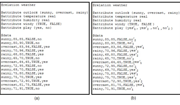
3.4 weather.arff dataset: (a) two-class , (b) transferred multi-class . . . . 32

3.5 Look-up table . . . 32

3.6 The process of applying ECOCs to a binary-class dataset . . . 34

4.1 An example of output code design (1-vs-all) . . . 36

4.2 OpenCL platform model . . . 47

4.3 OpenCL execution model . . . 48

4.4 A snippet of kernel code for random number generation . . . 49

4.5 Overview of the program flow chart . . . 50

4.6 GPU vs CPU . . . 51

4.7 A short snippet of JavaCL code . . . 54

5.1 AdaBoost: number of clusters vs. number of significant wins . . . 59

(13)

(14)

List of Tables

1.1 An example codeword matrix . . . 3

2.1 1-vs-rest . . . 9

2.2 Pairwise . . . 10

2.3 Example codeword matrix for four classes classification . . . 11

4.1 An example of an exhaustive matrix using Hamming distance . . . . 39

4.2 An example of a pre-defined random matrix . . . 44

5.1 Comparison of (a) AdaBoost and (b) multi-clustering with ECOCs using AdaBoost as the base learner, with 2, 3 and 4 clusters (i.e. 4, 6, and 8 classes in the transformed datasets) . . . 58

5.2 Comparison of (a) Bagging and (b) multi-clustering with ECOCs us-ing Baggus-ing as the base learner, with 2, 3 and 4 clusters (i.e. 4, 6, and 8 classes in the transformed dataset) . . . 60

5.3 Comparison of (a) RandomForest and (b) multi-clustering with ECOCs using RandomForest as the base learner, with 2, 3 clusters (i.e. 4, and 6 classes in the transformed dataset) . . . 62

5.4 Exhaustive codes vs. END (2 clusters per class in the multi-clustering approach) . . . 63

(15)

5.7 Exhaustive vs. Random codes in multi-clustering (AdaBoost + C4.5

as the base learner) . . . 67

5.8 Exhaustive vs. Random vs. ”pre-defined” with 4 clusters per class (AdaBoost + C4.5 as the base learner) . . . 68

5.9 The “pre-defined” method with different numbers of clusters . . . 69

A.1 Exhaustive vs END with Bagging as their base learner . . . 78

(16)

Chapter 1 Introduction

Machine learning has been widely used in many applications, such as weather pre-dictions, medical diagnosis and face detection. It is a field dedicated to finding ways to automatically extract information form data. It involves the design and develop-ment of algorithms that allow computers to learn and evolve behaviours based on empirical data.

The algorithms of machine learning allow one to make a prediction for a missing value in a dataset or for future data based on statistical principles. An important task of machine learning is classification, which assigns instances into one of a fixed set of classes. Classification learning involves finding a definition of an unknown functionf(x) (Dietterich & Bakiri, 1995) based on a training set consisting of known input/output pairs.

1.1 Multi-class classification

Unlike two-class classification, which assigns observations into one of 2 classes, the multi-class classification problem refers to assigning instances into one of k classes. Many publications have proposed methods for using two-class classifiers for multi-class multi-classification because two-multi-class problems are much easier to solve. The meth-ods include decision trees, k-nearest neighbour classification, naive Bayes, neural networks and support vector machines (Witten & Frank, 2005). Nevertheless,

(17)

de-composing multi-class problems into two-class problems is another approach, which may yield better performance. Based on decomposition, we can then use two-class classifiers for multi-class classification problems. There are several methods that have been proposed for such a decomposition. This thesis investigates empirically whether error-correcting output codes, one such method, can be profitably applied to two-class problems by artificially creating a multi-class problem using clustering. Let us briefly review the basic decomposition methods here. They will be dis-cussed in more detail in Chapter 2.

1.1.1 1-vs-all

1-vs-all (Rifkin & Klautau, 2004) is one of the simplest approaches to turn multi-class problems into two-multi-class multi-classification problems. Suppose we have k classes, then this method reduces the problem of classifying the k classes into k binary problems so that we have k binary learners for those k problems. The ith _learner

learns the ith _{class against the remaining} _k₋_{1 classes, where we treat the} _ith _class

as positive and the rest as negative.

At classification time, the classifier with the maximum output is considered the winner and we assign the class based on the classifier corresponding to this class. Even though 1-vs-all is very simple, Rifkin and Klautau (2004) point out that the performance of this approach is comparable to other complicated methods. I pro-vided careful parameter tuning for the underlying learning algorithm is performed.

1.1.2 1-vs-1

1-vs-1 (Allwein & Shapire, 2000) is another simple strategy to convert multi-class classification problems into binary classification problems. In this approach, each class is compared to each other class and the remaining classes are ignored. A

(18)

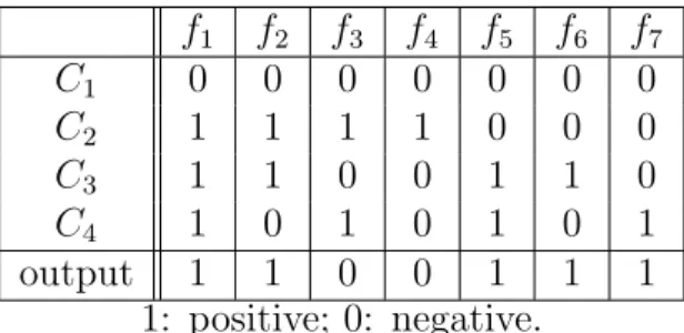
f1 f2 f3 f4 f5 f6 f7 C1 0 0 0 0 0 0 0 C2 1 1 1 1 0 0 0 C3 1 1 0 0 1 1 0 C4 1 0 1 0 1 0 1 output 1 1 0 0 1 1 1 1: positive; 0: negative.

Table 1.1: An example codeword matrix

binary classifier is built to discriminate between each pair of classes. For k classes, it requires k(k−₂ 1) binary classifiers.

At classification time, a voting is performed among the classifiers and the class that receives the maximum number votes wins. Allwein and Shapire (2000) state that this approach is generally better than 1-vs-all.

1.1.3 Error-Correcting Output Codes (ECOCs)

The ECOC (Sejnowski & Rosenberg, 1987) method was first pioneered by Sejnowski and Rosenberg in their well-known NETtalk system. It involves designing a dis-tributed output code matrix M. Each class is assigned a unique binary string of lengthn. We call this string codeword.

The number of classes is the number of rows in the matrix M and the length of the binary strings n is the number of columns in M. Then n binary functions are learnt, where the ith _{binary classifier learns the} _ith _column.

As an example, consider Table 1.1, which has 7 columns and 4 rows for a four-class problem. Note that each four-class has a unique codeword because each row is distinct. The columns can be chosen to be meaningful in a real world situation, but this is only possible if sufficient prior knowledge is available, and generally not the case. For example, in this thesis, we use all possible combinations of bits in the columns with the so-called exhaustive coding method. Regardless of the method used it is important that all columns are distinct to each other so that each binary

(19)

leaner learns a unique problem.

To classify an instance for which we do not know the class value, the seven binary classifiers f1, f2, ..., f7 are evaluated on this instance to obtain a 7 bits string, for

example 1100111. We then compute the Hamming distance of this string to each of the 4 codewords (rows). The codeword (class) who has the smallest Hamming distance is considered as the class label and output as the classification for the original multi-class problem.

The process of mapping the output string to the nearest codeword (class) is called decoding. The way that we define the matrix is call encoding. In this thesis, we will discuss some encoding and decoding methods in Chapter 2 and 4.

The measure of the quality of the codeword matrix is the minimum Hamming distance between any pair of codewords (rows). Suppose d is the minimum Ham-ming, then we can correct up to d−₂1 bit errors. Note that for this method to work, the errors of the classifiers should be correlated as little as possible so that they do not all make a mistake for the same instance. As a minimum, all columns in the matrix need to be distinct, so that the learning problems are different. Therefore, a good codeword matrix should satisfy two aspects:

Row Separation

We maximize the minimum Hamming distance between any pair of codeword.

Column Separation:

• All columns are distinct.

• There is no inverse from one to another

(20)

Note that this is the minimum requirement. Ideally, the Hamming distance between any pair of columns should also be as large as possible. How many bits of errors one can correct is given by row separation and how likely any two binary learners make similar mistakes is influenced by the column separation. We will cover more detail in Chapter 4.

1.2 Objective and motivation

We have discussed some multi-class classification strategies based on decomposition and we know that these techniques may yield high accuracy models, e.g., using ECOCs can often improve on applying a multi-class capable classifier directly to a multi-class dataset. However, we cannot use those techniques on two-class datasets without any further processing steps.

The objective of this thesis is to investigate whether ECOCs and similar methods can be profitably used for two-class classification problems. As ECOCs cannot be applied directly to two-class situations. The motivation of this thesis is to design and evaluate an approach to turn two-class problems into multi-class problems and then apply these multi-class techniques.

1.3 Thesis structure

Chapter 2 reviews the background on important concepts used in this thesis. It includes multi-class decomposition-based methods, i.e. 1-vs-all, 1-vs-1, ECOCs and ENDs. It also covers the machine learning algorithms that will be used in the experiments, such as C4.5, AdaBoost, Bagging and RandomForest.

Chapter 3 introduces clustering techniques that can be used for turning two-class datasets into multi-two-class ones, for example, simplek-Means andx-Means. This

(21)

chapter also gives detail on how to use these techniques in experiments with real classification problems.

Chapter 4 describes several decoding and encoding methods. Decoding methods include Hamming decoding, inverse Hamming decoding and Euclidean decoding. Encoding methods includes exhaustive coding, random coding and ”pre-defined” code found using random search. It also has a detailed discussion on GPU program-ming that we used to find good ”pre-defined” code matrices using random search.

Chapter 5 presents the datasets used for evaluation and the results of the exper-iments.

(22)

Chapter 2 Background

In machine learning, multi-class classification refers to assigning one ofkclasses to an input object. The classification of multi-class problems involves finding a function

f(x) whose range contains more than two classes. Compared to better understood two-class classification, which classifies instances into two given classes, multi-class classification is more complex and delicate. Many of the existing algorithms were originally developed to solve binary classification problems.

Some existing standard algorithms can be naturally extended to be used in multi-class multi-classification settings. Various techniques have been proposed. They include decision trees (Quinlan, 1993),k-nearest neighbours (L. & et al., 1996), naive Bayes (Witten & Frank, 2005) and support vector machines (Barnhill & Vapnik, 2002). On the other hand, decomposing multi-class classification into binary classification is a possible approach, which can be universally applied, and which may yield better performance. Based on decomposition, multi-class classification can be solved using output labels or probability estimates of standard two-class classifiers.

Decision trees learning is a well-know and powerful classification algorithm that can be directly applied to multi-class classification. It has been used in the research presented in this thesis in conjunction with ensemble learning methods, on behalf of other standard classification techniques to compare to the decomposition-based methods. In particular, C4.5 (Quinlan, 1993), which is implemented using Java in WEKA as J48 (Witten & Frank, 2005), is used to build decision trees for bagged

(23)

and boosted classifiers.

In this chapter, we will look at some of the existing algorithms that can deal with multi-class classification using decomposition. We will also look at the standard learning algorithms used for the experiments in this thesis: decision tree learning using C4.5, boosting, bagging and randomization.

2.1 Decomposition-based methods

Decomposing multi-class problems into binary problems is a popular way to deal with multi-class classification. In some case, the classification performance of these approaches is greater than that of applying a standard multi-class-capable learning algorithm directly, e.g. decision tree learning. In this section, we are going to review some of the existing decomposition-based methods.

2.1.1 1-vs-rest

A simple way to solve the problem of classifying k (k_>3) classes is to use the 1-vs-rest method (Rifkin & Klautau, 2004). k is the number of classes. In this approach

k dichotomizers (i.e. two-class classifiers) are learnt fork classes, where each learner learns one class against the remaining k−1 classes. For this approach, we require

n (n = k) binary classifiers. Each classifier treats the kth _{class as positive and the}

remaining k−1 classes as negative.

For example, for four classesA, B, C andD, we have four learnersf1,f2,f3 and

f4, where learner f1 learns class A against classes B, C and D, learner f2 learns

class B against classes A, C and D, and so on. See Table 2.1. The classifications in the training data are relabelled based on this scheme so that a standard learning algorithm can be used to learn four different classification models, each responses for identifying one class.

(24)

class A class B class C class D f1 1 0 0 0 f2 0 1 0 0 f3 0 0 1 0 f4 0 0 0 1 1: positive; 0: negative. Table 2.1: 1-vs-rest

When classifying a new instance, the class whose classifier produce maximum output, i.e. which is the most confident that the classification should be, is the winner and this class is assigned to the instance.

Although 1-vs-rest algorithm is simple, Rifkin and Klautau (2004) state that this approach provides performance that is comparable to other more complicated algorithms when the binary classifier is tuned well.

2.1.2 Pairwise classification

Pair-wise classification is also known as the 1-vs-1 algorithm or all-vs-all and it is another simple way to convert multi-class classification problems into binary clas-sification problems. The pairwise clasclas-sification algorithm requires that for a given numbers of classes, each possible combination of values for any pair of classes is covered by one classifier. Each binary classifier is built to discriminate between one pair of classes, while ignoring the rest of the classes. For k given classes, we thus have: N = Pk−1

i=1, where N is the number of required classifiers. Each classifier

treats one class as positive, another class as negative and the rest of the classes are ignored.

Assume that we have a dataset with 4 (k = 4) classes, then we have P4−1

i=1 = 6

classifiers. The 6 corresponding two-class problems can be described as in Table 2.2.

(25)

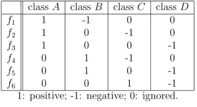
class A class B class C class D f1 1 -1 0 0 f2 1 0 -1 0 f3 1 0 0 -1 f4 0 1 -1 0 f5 0 1 0 -1 f6 0 0 1 -1

1: positive; -1: negative; 0: ignored. Table 2.2: Pairwise

As we can see from Table 2.2, f1 only learn two classes, A or B, for example.

Classes C and D are ignored. At classification time, a voting is performed among all the binary classifiers and the class who receives the maximum number of votes wins.

In practice, the pair-wise approach is generally better than the 1-versus-rest approach, but it builds more classifiers than one-versus-rest algorithm(Allwein & Shapire, 2000).

2.1.3 ECOCs

Applying Error-Correcting Output Code (ECOC) is another technique that com-bines binary classifiers in order to address a multi-class problem. The classification error rate of a learning algorithm can be decomposed into a bias component and a variance component, and it is known that ECOC can reduce the bias and variance of the base classifiers. ECOCs have been successfully applied to a wide range of applications in machine learning (Aly, 2005) .

The ECOC method involves designing a code matrix M for a given multi-class problem and each column in the matrix represents a bit column for one base learner. Assume that there are n columns for a k-class problems. We then have n base learners. The ith _{base learner aims to learn the} _ith _{column respectively so that} _n

(26)

f1 f2 f3 f4 f5 f6 f7 C1 0 0 0 0 0 0 0 C2 1 1 1 1 0 0 0 C3 1 1 0 0 1 1 0 C4 1 0 1 0 1 0 1 output 1 1 1 0 1 1 1 1: positive; 0: negative.

Table 2.3: Example codeword matrix for four classes classification

used to distinguish between thek classes.

Consider Table 2.3 as an example to explain how ECOCs work. f1, f2, ..., f7

are the base learners. C1, C2, ..., C4 are codewords. The row labelled “output” is

the predicted class of all base learners for a certain hypothetical test instance. In this case, there are 7 columns and 4 rows. The ith _{column is a learning scheme for}

the ith base learner. Each row represents one codeword corresponding to one class in the training dataset.

At classification time, when a new instance comes in, we use those 7 base learners to predict the class label. In our example, we receive the string 1100111. We then calculate the Hamming distance between each row and the output string 1100111. The row that has minimum Hamming distance to the output string is the predicted class label. In this case, class C2 has the smallest Hamming distance, namely 1.

Therefore, we assign the new instance to classC2.

In this example, the assumption is that classifier f4 made a mistake, which can

fortunately be corrected because the code matrix allows for this. The number of bits that can be corrected depends on the minimum Hamming distance between each pair of rows in the matrix. Details on this, and methods for designing good ECOC matrices will be discussed in Chapter 4 of this thesis.

(27)

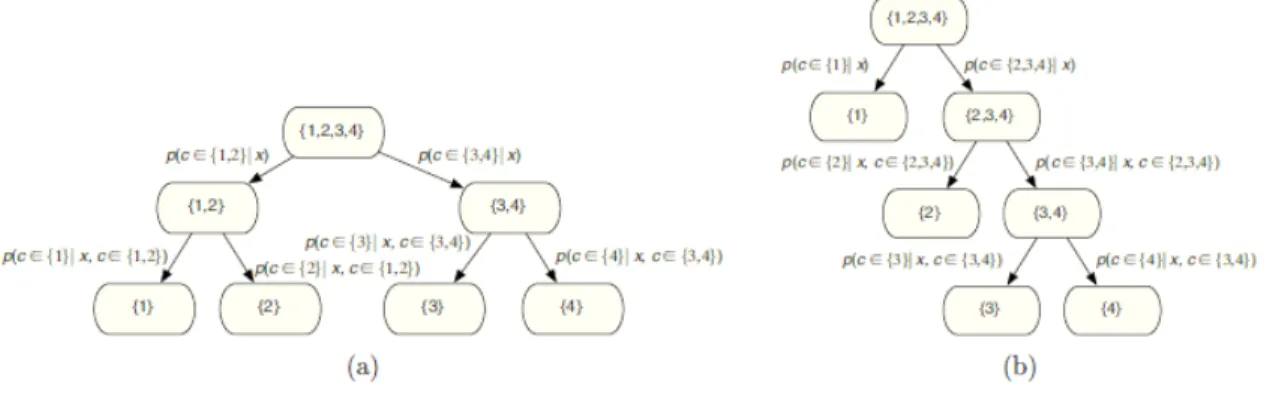
Figure 2.1: Two different systems of nested dichotomies, reproduced from END(Frank and Kramer, 2004)

2.1.4 END

Ensembles of Nested Dichotomies (END) were proposed by Frank and Kramer (2004). It is method that uses a tree structure to decompose a multi-class problem into binary classification problems. A nested dichotomies system randomly recur-sively splits a set of classes from multi-class classification into smaller and smaller subset (Frank & Kramer, 2004).

Nested dichotomies can be described as binary trees. A root node contains all classes and a leaf node only contains one class. At each node, the tree divides the set A into two subsets B and C that contain all the classes in set A. There are different possible ways to split a node. Figure 2.1 shows an example of two possible ways of constructing the binary trees for a four-class problem.

Classifiers are learned for the internal nodes of the tree. The estimated class probability distribution for the original multi-class problem can be obtained by multiplying the the probability of all the internal nodes that need to be visited to reach the leaf. For example, the probability of class 4 for an instancexis given by:

(28)

p(c= 4|x) = p(c∈2,3,4|x)×p(c∈3,4|x, c∈2,3,4)×p(c∈4|x, c∈3,4) based on Figure 2.2b

Both trees are valid class probability estimators. However, the estimates ob-tained from different trees are normally different. Frank and Kramer state that there are 3n₂n+1₋_{1 possible two-class problems for an}_n_{-class dataset. In this}

four-class example, therefore there are 25 different ways to build the binary trees. This number grows extremely quickly since the term 3n arises. It becomes a problem that it is impossible to generate all trees exhaustively. Hence, Instead of doing an exhaustive search, the END method evaluates the performance of ensembles of ran-domly generated trees, where probability estimates from different trees are simple averaged.

According to Frank and Kramer, ensembles of nested dichotomies produces more accurate classifiers than applying C4.5 to multi-class problem directly. Frank and Kramer also point out that this approach produces more accurate classification models than pair-wise algorithm if both techniques are applied with C4.5. Compared with error-correcting output codes, it has similar performance.

2.2 Tree and ensemble learning

In this section, we review the algorithms that are used in our experiments, namely C4.5(Quinlan, 1993) , AdaBoost (Freund & Schapire, 1995), Bagging (Breiman, 1996) and RandomForest (Ho, 1995). C4.5 is used as the base learner of AdaBoost and Bagging. AdaBoost is a popular and efficient boosting algorithm and it combines many “weak” learners as one ”strong” learner. Bagging is a short word for bootstrap aggregating. RandomForest is an ensemble meta-algorithm that consists of many decision trees that are generated using a partially randomized decision tree learner.

(29)

2.2.1 C4.5

C4.5 (Quinlan, 1993) is one of the most well-known decision tree algorithms. It is an extension of the earlier ID3 algorithm also developed by Ross Quinlan. J48 is an open source Java implementation of C4.5 in the WEKA data mining tool (Witten & Frank, 2005). Since J48 is used as the based learner for most of the experiments in this thesis, it is very important to understand the approach that it uses to construct a decision tree as well as the strategy of pruning the tree.

Constructing the decision tree

C4.5 uses ”divide and conquer” to build a decision tree using dataset T. There are three possibilities of constructing a decision tree from a set T of training data of k

classes {C1, C2, ..., Ck} (Quinlan, 1993):

• T contains one or more instances that have the same classCj. In other words,

all the instances belong to a single classCj, and a leaf node should be created

for them..

• T contains no instance. In this situation, the decision tree is a leaf. The class of the instances in the leaf must be determined from information other than

T. C4.5 uses the most frequent class at the parent of this node.

• T contains instances that belong to a mixture of classes. In this case, the decision tree is not a single leaf normally. The idea is to splitT into subsets of instances. C4.5 chooses a test that is based on a single attributes to generate mutually exclusive outcomes {O1, O2, ..., On}. T is then split into subsets

T1, T2, ..., T n, where subset Ti has all instance in T that have outcome Oi.

Constructing a decision tree can be done recursively based on the above three possibilities. The basic algorithm is to select an attribute to use at the root node

(30)

to split the instances. For each possible values of the attribute, we create a branch and then assign all the instances to the different branches. We repeat the process for each branch using only the instances that reach the branch. We stop the process when all instances in one branch have the same classification or where there are no instances left.

Now the question is what attribute we select when splitting instances. Informa-tion gain is widely used. LetAttrbe the set of all attributes and T be the set of all training instances. value(x, a) with x∈T defines the value of a specific instance x

for attribute α ∈ Attr, and H(s) specifies the entropy of the class distribution in subsetS of T. The information gain for a given attribute α∈Attr is calculated as follows: Inf ormationGain(T, a) =H(T)−P v∈value(a) |{x∈T|value(x,a)=v}| |T| H({x∈T|value(x, a) =v})

We calculate the information gain for all attributes and choose the one that gains the most information to split on.

Pruning the decision tree

If the decision tree overfits the training data, the performance will get worse. Hence it is important that we prune the tree to produce a simpler tree that is more robust with respect to variance in the training data. There are two basic ways that can be used to modify the tree: prepruning (or forward pruning) and postpruning (or backward pruning).

Preprunning involves trying to decide not to divide a set of training instances any further. Preprunning is more efficient because time is not wasted on assembling

(31)

structure that is not used in the final tree. However, we need to have a measure to stop splitting a subset. The measures that have been used include information gain, error reduction or statistical significance (Witten & Frank, 2005). For example, in a subset, if the assessment is smaller than a particular threshold value, the division is stopped. However, Breiman (Breiman & et al., 1984) point out that it is not always easy to find the right stopping value. If the threshold is too high, it reduces the accuracy due to underfitting, while if the threshold is too low, the tree may overfit the data.

Postpruning builds the complete trees first and then remove some of the struc-ture. The C4.5 decision tree algorithm uses postpruning to prune trees. Quinlan (1993) states that preprunning is quite satisfactory but uneven in some domains. The postpruning process is to develop a completed and overfitted tree and then prune the tree. Trees are normally pruned by replacing one or more sub trees with leaves. The class of the leaf can be determined by examining the training instances covered in the leaf and identifying the most frequent class. Subtree replacement works from the leave nodes back up toward the root node. This approach is quite simple. First, replace the child nodes with a single leaf node. Then continue to work back from the leaves. We prune the tree until the decision is made not to.

Subtree raising is more complex and is also used by C4.5. With the subtree rais-ing operation, we raise the subtree and replace its parent node. Then we reclassify the instances in the other branch of the parent node into one of the leaf nodes in the raised subtree. The general procedure is the same as for subtree replacement, we prune the tree until the decision is made not to

These two pruning methods require a decision whether to replace an internal node with a leaf for subtree replacement, and whether to replace an internal node with one of the nodes below it for subtree raising. To achieve this, we need to estimate the error at the internal node and the leaf nodes. The decision can be

(32)

made by comparing the estimate error between the un-replaced/un-raised trees and replaced/raised subtrees. C4.5 uses the upper limit of a confidence interval for the error on the training data as the error estimate.

2.2.2 Adaboost

Adaboost, short for Adaptive Boosting, is a machine learning algorithm that con-structs a “strong” classifier as a linear combination of “simple” and “weak” clas-sifiers. It was formulated by Yoav Freund and Robert Schapire (1995). Adaboost is one of the most popular machine learning algorithms. The idea is quite intrigu-ing: It generates a set of weak classifiers and simultaneously learns how to linearly combine them so that the error is reduced. The result is a strong classifier built by boosting the weak classifiers. Therefore, AdaBoost can be used in conjunction with many other machine learning learning algorithms to improve the accuracy of learning models. The algorithm of AdaBoost is shown in Figure 2.2.

First we initialise m all training instances to have equal weight. In each iteration of the algorithm, based on the current weighted version of the data, we learn a classifier Ck. Then we increase the weight of training instances if they are

misclassified by classifier Ck and decrease an instance’s weight if it is correctly

classified byCk.

The weight for iterationk+ 1 are calculated as follows:

Wk+1(i) = Wk(i)e−αkyiCk(xi) Zk , where αk = 1₂ln[ (1−Ek) Ek ], and Zk = Σmi=1Wk+1(i).

(33)

Note the following:

• The class value yi of training instance xi is assumed to be either -1 or 1, and this also holds for the classification Ck(xi).

• The Ek error is calculated based on the summation and normalization of all wrongly classified weighted training instances by the weak learner Ck. The

weak learner should be better than random guess Ek<0.5.

• The measurement αk measures the importance assigned to Ck. Note that α >= 0 ifE <= 1₂ and α gets larger whenE gets smaller.

• Zk is a normalization factor so that Wk+1 will be a distribution.

At classification time, the classifiers Ck are linearly combined using the

impor-tance factor αk. Therefore, for any given input training dataset, we can describe

the final classifier as:

H(x) = sign(PK

k=1αkCk(x))

AdaBoost often produces classifiers that are significantly more accurate than the base learner (Witten & Frank, 2005), and it does not require prior knowledge of the weak learner. The performance is completely dependent on the learner and the training data. Note that AdaBoost can identify outliers based on their weight. It is susceptible to noise with very large number of outliers. In practical situations, it can sometimes generate a classifier that overfits the data and produce a significantly less accurate one than a single weak learner.

(34)

Initialize

Dataset : D={ x1 ,y1 ;...; xm, ym };

Iterations: K;

Weight: W1(i) = _m1, i= 1, ..., m, wherem is number of instances.

Assign equal weight to each training instance. Iterations

For k = 1 toK

Train weak learner Ck using weighted dataset Dk sampled

according to Wk(i).

Compute error Ek of the model based on dataset Dk.

For each instance in dataset:

If instance classified correctly by model: Decrease weight of training instance. If instance misclassified correctly by model:

Increase weight of training instance. Normalise weight of all instances.

Figure 2.2: Adaboost Algorithm

2.2.3 Bootstrap aggregating (Bagging)

Boosting and bagging (Breiman, 1996) both adopt a similar approach that combines the decisions of different models to create a single prediction. But they derive the individual models in different ways. In boosting, we modify the weight of instances according to their classification based on whether it is correct or not, while in bag-ging, all models receive instances of equal weight but differently sampled datasets.

Bagging is a meta-algorithm that uses several training datasets of the same size to improve stability and classification accuracy. The training datasets are randomly chosen from the original training data. The algorithm is described in Figure 2.3.

For a given datasetDsize ofn, bagging generatesmnew training datasets Di of

the same size. Each new datasetDi is generated by sampling examples fromDwith replacement. By sampling with replacement, it is likely that some instances may be chosen more than once. Statistically, set Di is expected to have 63.2% unique

(35)

model generation

Let n be the number of instances in the training data, For each of t iterations

Samplen instances with replacement from training data. Apply the learning algorithm to the sample

Store the resulting model

classification

For each of the t models:

Predict class of instance using model. Return class that has been predicted most often

Figure 2.3: Bagging Algorithm

training dataset.

Bagging reduces variance and helps to avoid overfitting. It helps most if the underlying learning algorithm is unstable, which means a small change in the input data can lead to very different classifiers, since the classification of Bagging is ob-tained by averaging the output or by voting. Because it averages several predictors built from similar training datasets, bagging does not improve very stable algorithms like k-nearest neighbours.

2.2.4 Random forest

A random forest is also an ensemble meta-algorithm and consists of many decision trees. The term random forest comes from the term random decision forest, which was proposed by Tin Ho of Bell Labs in 1995. It combines the bagging idea and the random selection of features in order to construct a collection of decision trees.

The selection of a random subset of attributes is an example of the random subspace method that is also called attribute bagging (Ho, 1995). In random forest, a different random subspace is chosen at each node of a decision tree. A standard attribute selection criterion such as information gain is then applied to choose a

(36)

model generation

LetN be the number of instances in the training data, and

M be the number of attributes of the instance. For each tree:

A m Training dataset is chosen by randomly selecting n (n < N) time from allN

training instances with replacement like in bagging.

Use number of attributes to determine the decision at a node of the tree, where m should be much smaller than M (m < M).

The rest of the instances are used to estimate the error of the tree.

For each node of the decision tree, randomly choose m attributes, and then calculate the best split based on these m variables in the training set. All individual trees are fully grown and not pruned

classification

Iterate over all trees in the ensemble;

and the average vote of all trees is the prediction of random forest

Figure 2.4: Random forest algorithm

splitting attribute based on this subspace. For each individual decision tree, the algorithm that is used for constructing trees is described in Figure 2.4.

The random forest algorithm is one of the most popular learning algorithms. In practice, it often produces highly accurate classifiers. Random forest is also very efficient regarding running time. It can handle large input data with very high dimensionality. The disadvantage of random forest is that it overfits some datasets with noisy classification (Ho, 1995).

(37)

(38)

Chapter 3 From two to many classes using

clustering

The goal of this thesis is to investigate whether Error-Correcting Output Codes (ECOCs) and similar methods can be profitably used for two-class classification problems. However, an immediate obstacle is that ECOCs cannot be applied directly to two-class situations. The problem is that we can correct only d−₂1 (rounded down) errors with the ECOC prediction scheme when the row separation (he minimum Hamming distance between pairs of rows) is d. Suppose that there are k classes. With exhaustive ECOCs, which deliver maximum possible error correction, and which will be discussed in detail in the next chapter, the number of columns in the code matrix is n = 2k−1 ₋_{1. Moreover, the pairwise Hamming distance between}

rows isd= 2k−2_{. This means we can correct up to}_x_{= 2}k−3₋_{1 bit errors. Therefore,}

we need to have at leastk _>4 classes to be able to correct 1 bit error. In that case, we can still get the correct classification even if one base learner misclassifies an example . In contrast, here is no guarantee that we can get the correct classification if one of the base learners makes an incorrect decision in a situation with less than four classes (k < 4). Therefore, we cannot the apply ECOC algorithm on 2 or 3 class-classification problem directly.

To be able to apply ECOCs on two-class or three-class datasets we need to develop an algorithm to turn the problem into a situation where there are more

(39)

than 3 classes (k > 3). The basic idea of our approach is quite simple. With the binary-class datasets in hand, we first transfer them to multi-class ones by creating clusters within each class, and then we can apply ECOCs on the transformed multi-class dataset at training time. At multi-classification time, we then transfer the output of the ECOCs models back to one of the original binary classes. To be able to transfer the ECOCs’ output to the final classification, we have to keep a look-up table to store the reference of which clusters were generated from which class. By transferring the binary dataset to a multi-class one and then applying ECOCs to it, we can hopefully improve the accuracy of classification models.

In this chapter we are going to look at some existing techniques, namely clus-tering and k-means, as well as our approach in detail. When we review the existing clustering techniques, we focus on how they cluster instances and the discussion of the parameter settings. Our approach includes how to use these techniques to turn two-class problems into multi-class classification problems in order to be able to apply ECOCs algorithm indirectly. We also list the detail of how we transfer the binary-class dataset to a multi-class dataset at training time and why this approach can potentially improve the performance of the classification models. Note that three-class problems can be dealt in the same way as two-class ones so that we only consider two classes as our example here to explain the process and the algorithms.

3.1 Clustering

Clustering is an existing technique that can be used to group instances in machine learning. It is a simple and straightforward approach that has been used for many decades. Clustering techniques are normally applied when there is no class that needs to be predicted but rather when the instances are to be divided into natural groups. We will use the idea of this approach to group instances in our algorithm.

(40)

Figure 3.1: An example of clustering expression

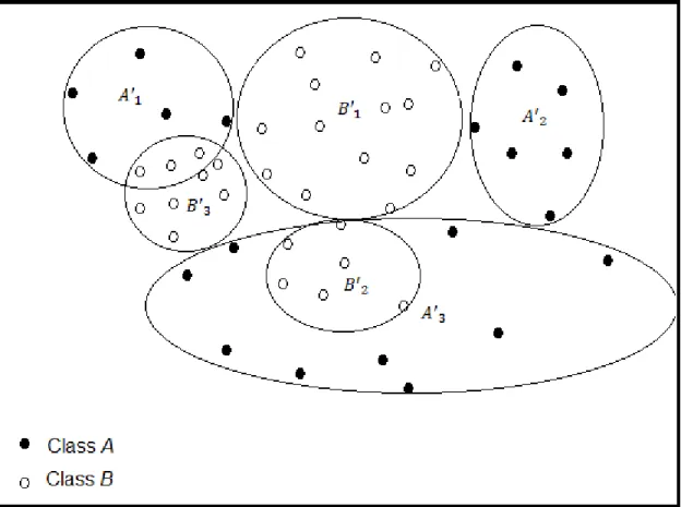
There are many different ways that can be expressed to cluster instances. Figure 3.1 show an example of a clustering expression, where data from 2 classes has been split into three clusters each, to create a six-“class” problem. There are a few possible different situations. First, the clusters may be overlapping so that an instance will fall in several groups. The clusters may be exclusive in which case an instance only belongs to one group. There are also some other situations where they may be probabilistic or they may be hierarchical.

The experiments in this thesis are based on the WEKA software. There are several different clustering algorithms that are available in WEKA, such as simple

k-Means (Witten & Frank, 2005) and x-Means (Witten & Frank, 2005) . k-Means is a classic clustering techniques and is simple and effective. x-Means is k-Means

(41)

extended by an method to automatically find the appropriate number of clusters. Instead of generating a fixed number of clusters,x-Means attempts to split a cluster into sub-clusters. Inx-Means, the decision between the children of each cluster and itself is done by comparing the Bayesian Information Criterion (BIC) values of the two structures.

For the experiments in this thesis, we want to see how different numbers of clusters affect our final classification models. Hence simple k-Means is used to cluster instances in the research presented here, and in this chapter, we only look at k-Means in detail.

3.2 k

-Means

k-Means is a classic clustering algorithm and it uses a distance function like instance based learning algorithms, for example IBK in WEKA. It is an algorithm that is very popular and easy to understand. k is a parameter that we need to specify to indicate how many clusters we want to build. After we build the k clusters using the given dataset, when an instance needs to be clustered using k-Means at clustering time, it assigns the instance to its nearest cluster (one of those k clusters). By nearest cluster, we mean the cluster that has the smallest Euclidean distance from its mean to the new instance. The output of k-Means consists of k groups of instances.

3.2.1 The algorithm

The training algorithm of k-Means is quite simple. Firstly, we need to specify how many clusterskwe want, as mentioned above. Thenk-Means chooseskinitial points as the cluster centres randomly. All instances in the dataset are assigned to their closest cluster centre using ordinary Euclidean distance as the measure. Next, we calculate the centroid (mean) of the instances in each cluster. Those centroids are

(42)

used as the new centre values for their respective clusters. All processes are repeated with the new cluster centres until the same points are assigned to each cluster in consecutive rounds. Finally, k-Means converges to a stabilized cluster centres and these centres will remain the same (Witten & Frank, 2005) .

k-Means is effective. Choosing the cluster centres to be the centroid minimizes the total squared distance from each of the cluster’s points to its centre. Once all cluster centres have stabilized, all instances are assigned to their closest cluster cen-tres. The overall effect is to minimize the total squared Euclidean distance from all instances to their cluster centres. According to Witten and Frank the minimum is a local one and there is no guarantee that it is global minimum. Different initial clus-ter centres can lead very different final clusclus-ter models. In other words, a completely different clustering can arise when there is a small change in the initial random choice. To address the problem, we can run the algorithm several times with differ-ent initial choice to find a good final cluster arrangemdiffer-ent. The final chosen result is the one with the smallest total squared Euclidean distance.

There are two issues that we may consider with k-Means. Firstly, k-Means may fail to find good cluster arrangements. This problem can be solved by running k -Means several times. Secondly, there is processing time required for finding the

k cluster centres. We can borrow the ideas of kD-Trees (Witten & Frank, 2005) and ball-Trees (Witten & Frank, 2005) that are used in instance based learning algorithms. They are faster distance calculating algorithms. However, the simplek -Means clustering algorithm in WEKA does not use these two techniques by default and using these more sophisticated techniques was not necessary for the experiments presented in this thesis.

(43)

3.2.2 Choosing the parameter

k

(the number of clusters)

The parameterk indicates how many initial cluster centres we want to have as well as the number of final clusters. As the experimental results presented in this thesis will show that it is important to specify an appropriate value to it. In particular, when we transfer a two-class dataset into a multi-class dataset, k is the coefficient that is used to multiply the number c of classes in the original dataset (c = 2 in binary data). The number of classes in the new transferred multi-class data can be defined as follows:

N =k×c, where

N is the number of new classes in the transferred dataset.

k is the number of clusters.

cis the number of classes in the original dataset.

Different values ofkcan generate different numbers classes in the newly generated multi-class dataset. For example, let:

k = 3 and c= 2. Then we have

N =k×c= 6 classes

Since N = 6 and this is greater than 4, the ECOC method can then successfully be applied to this new dataset. We are going to dive into more detail on this in Section 3.3. We know that k is an important parameter as different values ofk lead to different codewords matrices. In principle, the larger the k value is, the more errors we can correct using the ECOC method. In practice, however, finding a good

(44)

codeword matrix is becoming very costly when the value of k gets larger. In the experiments presented in this thesis, the value ofk is in the range k ∈ {2,15}. We will discuss how to find good codeword matrices in Chapter 4 .

3.3 Turning two-class problems into multi-class

ones

Because we can only apply ECOCs on multi-class classification problems and more specifically ECOCs require that the dataset has at least four classes to be able to correct at least one bit error, it is necessary to transfer two-class data into multi-class data to be able to apply ECOC at training time. At classification time, we change the obtained classification back to corresponding classes in the two-class dataset.

3.3.1 Creating a multi-class dataset

When we apply ECOC algorithms on binary class problem, clustering (k-Means) is a natural way to turn the two-class dataset into a multi-class dataset. To keep the problem simple, we use the same number of clusters for each class in the dataset.

Suppose we have two classesAandBin our binary datasetT and the distribution of datasetT is shown in Figure 3.2.

If we specify 3 as the number of clusters for each class for example, we will end up with a 6-class dataset. The new classes are:

A₁0, A0₂, A0₃, B₁0, B₂0 and B₃0, where

A0₁, A0₂ and A0₃ are generated from A, and

B₁0, B0₂ and B₃0 are generated from B.

The new class label of an instance in the new dataset T0 will be one of these six classes. The new clustered dataset T0 will be our training dataset. The new

(45)

Figure 3.2: An example of 3 clusters per class for a two-class dataset

dataset T0 can be generated using the algorithm described in Figure 3.3, assuming the clustering technique has already been applied to find the k clusters per class, which can be done by running k-Means on the data of each class separately.

The created dataset T0 has the same number of instances as original dataset T. There are also the same number of attributes and the same attributes values. The only difference is that there are more classes in T0 than T. More specifically, the number of classes inT0 is the product of the number of classes in T and the number of clusters k we specified when we created T0 using clustering. Therefore, the more clusters (larger k values) we provide, the more classes we will end up with in our new dataset T0. Figure 3.4 shows an example of T and T0 with k = 2.

(46)

Steps:

1. Build instances set T0 with empty data in it that has the same structure as T but k×2 class values.

2. Iterate over all instances in the original binary class dataset T. 3. For each instance i inT:

4. Create a new instance i0 with attributes in which values are copied from the instance i.

5. Find the closest cluster center for instance i and get the new class value (one of the clusters, for example, A0₁, A0₂ orA0₃, when the original class is A). Assign the cluster value to the new instance i as its new class label.

6. Store the new instance i0 inT0.

7. Repeat step 4, 5, 6 until iteration is finished.

Figure 3.3: The process of creating a multi-class dataset

the key: we always turn the binary-class into a multi-class problem classification before using ECOCs. So rather than using dataset T, we are using dataset T0 as our training data to build classification models. The prediction of those models will be one of these classes in datasetT0. In fact, the classification is one of the clusters. In the next two sections, we are going to look at how we can use these classification models to produce the final output.

3.3.2 Look-up table

When we transfer the binary-class dataset T into a multi-class dataset T0, we do not want to lose the connection between T and T0. Therefore, we create a look-up table to keep a reference of the classes in T and T0. Figure 3.4 is an example of a look-up table with i clusters.

This look-up table is very important even though it is not necessary to have it at training time: we do not need to worry about this table when we build classification models. It will only be used for producing the final binary classification. At the time of outputing the final decision, the classification models based onT0 will only

(47)

Figure 3.4: weather.arff dataset: (a) two-class , (b) transferred multi-class A0₀, A0₁,· · · , A0_i | {z } A B₀0, B₁0,· · · , B_i0 | {z } B

Figure 3.5: Look-up table

predict the classes in T0, for example, A0₂, A0₃ or etc. This look-up table holds a reference so that we can transfer the classification A0₁ or A0₃ back to the original A

later.

3.3.3 The classification

We have already talked about how we turn the two-class datasetT into a multi-class dataset T0 so that we apply ECOCs to T0 in order to improve the accuracy of the classification models. This is the first step: we have created the required training dataset (with at least four classes to be able to correct at least one bit error).

With the dataset T0, we can use whatever base learner in ECOCs to learn clas-sification models. As we mentioned before, these models will produce one of the

(48)

clusters, which is not the final output. We need to have a way to transfer the out-put of ECOC models to be one of the binary classes in the original datasetT. After we have transferred these clusters into classes, we will get the final classification.

The algorithm for transferring the output of the ECOC model to the final clas-sification can be very simple. Assume that the output of the ECOC model is A0₁, one of the classes in the generated multi-class dataset. We simply assign the final predicted class to classA. The reason is thatA0₁ is one of the clusters split fromA. This process is done using the reference in the look-up table that we created when we generated the training dataset.

3.4 Overview of the clustering approach

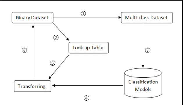
We have discussed the process for turning two classes to many classes using cluster-ing. It is useful to draw all these process in one graph so that we can easily navigate and understand. Figure 3.6 shows the whole process.

We summarise the process using the following steps:

• 1. Use clustering approach to transfer the binary-class data into a multi-class one;

• 2. Save a look-up table to store the reference;

• 3. Learn classification models using ECOC method;

• 4. Classify instance;

• 5 and 6 Use the look-up table to produce the final class label.

Note that we only consider the case where we cannot use ECOCs directly, i.e., binary datasets and three-class datasets. Actually this approach is not limited to two-class and three-class problems. It is available to be applied on multi-class data

(49)

Figure 3.6: The process of applying ECOCs to a binary-class dataset

if we want to have more classes in the training set. However, this scenario is beyond the scope of this thesis.

(50)

Chapter 4 Generating and using ECOCs

It is known that the lowest error rate is not always reliably achieved by applying a single classifier for some classification problems. That is the reason why using an Error Correcting Output Code (ECOC) was proposed as a combination of binary problems to address multi-class problems. We have discussed some background of ECOCs in Chapter 2 and we know that the ECOC technique is widely applied in many applications. In this chapter, we consider the principle and the usage of ECOCs.

The ECOC technique involves two distinct stages: encoding and decoding. For a given set of classes, the encoding method builds a codeword for each class. The decoding process uses the codeword matrix to produce an output code. The output codeword string can be used to make a classification decision for a given test sample.

4.1 Encoding method

At the encoding stage, suppose we have k classes that need to be learnt for a given dataset T, then n different learners are trained in the ECOC ensemble. In other words, n dichotomizers need to be trained. A codeword of length n is obtained for each class, where the ith bit of the code corresponds to the ith dichotomizer. The code is composed of 0s and 1s for binary problems.

(51)

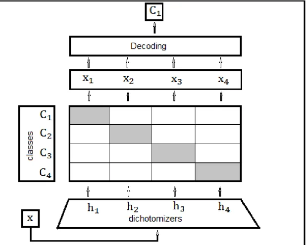
Figure 4.1: An example of output code design (1-vs-all)

{1,0}k_×_n_{. Figure 4.1 shows an example: the so-called one-vs-all method which is}

one of the simplest choices for the output code. Here, 1s are marked as grey cells and 0s as white ones. Note that this one-vs-all matrix is not actually error-correcting and just used as an example.

We also can add another symbol, namely −1, to the matrix which now contains

{1,0,−1}. In this case, we treat 1 as positive, −1 as negative and 0 as ignored, e.g. we can represent the pairwise method that we mentioned in the chapter 2. We will introduce two more encoding methods in this chapter, namely exhaustive and random, which we will consider in detail in Sections 4.3 and 4.4.

(52)

4.2 Decoding methods

The decoding process is to apply then binary classifiers and then obtain an output codexfrom the learners. This output code is used to compare to the base codewords (rows) that are defined in the matrixM. The new instance is assigned to the class with the closest codeword. The most frequently decoding designs are: Hamming Decoding, Inverse Hamming Decoding and Euclidean Decoding.

4.2.1 Hamming decoding

The Hamming decoding method is based on measurement of Hamming distance and it is one of the most common decoding techniques. The experimental results in this thesis are based on Hamming decoding method. In this section, we will give a brief introduction of Hamming distance and then we will state how the Hamming decoding method has been used.

Hamming distance

We have a short review of the Hamming distance here. Hamming distance was first introduced by Richard Hamming in 1950. It is used in telecommunication to detect and correct flipping errors. In machine learning, the term Hamming distance between two equal length words is the number of different bits at the same position where the corresponding symbols are different. In other words, it describes the minimum number of substitutions need to change from one word to the other word. To calculate the Hamming distance between two words is quite simple. The Hamming distance calculation can be processed as follows (suppose there arek bit symbols in each string):

(53)

• Iterate i from 0 tok.

• Compare the symbols at the ith position in both strings.

• If they are different.

increase counter d by 1

• Stop when we reach the last bit of the string.

Hamming distance represents the distance between two strings. In other words, it is the number of different bits in two strings. For example, the Hamming Distance between:

”apple” and ”apply” is 1;

”10010011” and ”01011111” is 4; ”10101010” and ”01010101” is 8.

Hamming distance can be used for any string of symbols. However, in this thesis, the examples are binary cases so that most strings are composed of 0s and 1s.

Hamming decoding method

The Hamming decoding method (Hamming, 1950) is one of the most popular strategies for ECOCs. From its name, it is obvious that the initial proposal to decode is to use the Hamming decoding measure. There is an alternative way to calculate Hamming Distance. It is defined as follows:

HD(x, yi) =Pn_j₌₁(1−sign(xjyij))

The Hamming decoding method is based on the error correcting principle under the assumption that two possible symbols can be found at each position of the sequence. Each learning task can be modelled as a binary problem.

(54)

f1 f2 f3 f4 f5 f6 f7 class A 0 0 0 0 0 0 0 class B 0 0 0 1 1 1 1 class C 0 1 1 0 0 1 1 class D 1 0 1 0 1 0 1 output 1 0 1 1 1 0 1

Table 4.1: An example of an exhaustive matrix using Hamming distance

Hamming decoding can guarantee to correct up to d−₂1 bit errors, where d is the minimum Hamming distance between all possible pairs in the codeword matrix. Suppose we have the following codeword matrix:

Heref1, f2, ..., f7 are the base learners. These learners can be any binary learners

as they learn to discriminate between 0s and 1s. For example, f1 learns class D

against class A, class B and class C. In the output example in the table, the prediction of f1 is positive so that the output for f1 is 1. This is a very clear case.

Learnerf3 is a little bit different. It learns classC and class D against classA and

class B. In other words, f3 predicts whether the class belongs to either class A and

classB or class C and class D. In this example, the prediction of f3 is also positive

(1). We keep tracking the classifiers f1, f2, ..., f7 and then we get the output code

string 1011101.

With the output code string 1011101 in hand, we then calculate the Hamming distance to each base codeword. The class with the smallest Hamming distance is the predicted class. In our example, the Hamming distances to each base codeword are:

class A: 0000000 vs 1011101 is : 5 class B: 0001111 vs 1011101 is : 3 class C: 0000000 vs 0110011 is : 5 class D: 1010101 vs 1011101 is : 1

(55)

test instance to class D. The Hamming distance can be calculated using either of those two ways that we mentioned before.

4.2.2 Inverse Hamming decoding

Inverse Hamming decoding (Escalera & Pujol, 2010) is another popular decoding method. It is defined as follows: Let ∆ be the matrix composed by the Hamming decoding measure between the codewords. ∆ can be inverted to find the vector containing the N individual class likelihood function by means of:

IHD(x, yi) =max(∆−1DT) where,

∆(i1, i2) =HD(yi1, yi2), and

D is the vector of Hamming decoding values of the test codeword x for each of the base codewords yi.

Escalera and Pujol state that, in practical situation, the behaviour of the inverse Hamming decoding method is very close to the behaviour of the Hamming decoding strategy.

4.2.3 Euclidean decoding

Euclidean Decoding (Escalera & Pujol, 2010) is another well-known decoding strategy. This measure is defined as follows:

ED(x, yi) =

q Pn

j=1(xj−yij)

2

It measures the Euclidean distance between two code vectors, It also behaves similarly to the Hamming distance.

(56)

4.3 Exhaustive encoding method

We have talked about several encoding methods already, e.g. vs-rest and one-vs-one. In this section, we consider a powerful method: the exhaustive method. The exhaustive method builds a codeword matrix that contains all possible unique codewords.

Suppose that there arekclasses. The number of columns in an exhaustive ECOC is n = 2k−1 −1. This means that the length of the codeword is n. Each column represents one base learner. Table 4.1 is an example of exhaustive method. Table 4.1 is an example of the exhaustive method.

It is quite simple to generate the matrix. We know that there should be k rows andn columns. We first build n binary strings of lengthk. The value of the binary strings starts from 1(in decimal). For example, suppose we have

k = 4 classes, then we have

n= 2k−1₋_{1 = 7}

The exhaustive matrix should have 4 rows and 7 columns. We write 7 binary strings of length 4 whose decimal value starts from 1 (in decimal). We have:

string 1: 0001 string 2: 0010 string 3: 0011 string 4: 0100 string 5: 0101 string 6: 0110 string 7: 0111

(57)

With these 7 strings matrix in hand, we can easily create our exhaustive matrix. All we need to do is to turn the matrix 90◦C clock wise. We then have our exhaustive matrix: 1234567 0000000 1111000 1100110 1010101

This process is simple and straightforward. In an exhaustive matrix, each row represents one codeword for one class as in other output-code-based approaches. As we mentioned before for k class datasets, we have k rows and 2k−1 ₋ _{1 columns}

(number of base learners).

Generating an exhaustive ECOC does not require a very intelligent codeword matrix generation design. The process is very easy to follow. In practice, it is a strong method because it uses the maximum number of possible unique base learners. That means it learns all possible binary combination problems.

The exhaustive method is a great approach to use in ECOC-based classifica-tion. However, the codeword matrix becomes very large when the number of classes increases. This is because the number of columns is 2k−1₋_{1 and will increase}

ex-ponentially quickly. As a result, the time that is consumed for training the base learners becomes a big issue.

If the number of classes is very large, it is quite impossible to run the experiment. Based on experience with the experiments presented in this thesis, the number of classes can go up to about 8. In this case, we have 127 base learners. Even though exhaustive ECOC work very well, we need to consider another strategy to handle a situation where there are many classes.

(58)

4.4 Random method

Because of the limitation of running the exhaustive method, we can use a very simple, so-called ”random” method to cover situations that the exhaustive method cannot handle. In this section, we are going to look at one of the random methods that have been used in this thesis. We have used two random methods in this thesis. One is WKEA’s existing method and the other is a newly developed one. We can treat the one in WEKA as a purely random method. It simply creates a random code matrix by setting bits based on unbiased coin tosses. In this section, we focus on our newly method that generates an optimized pre-defined matrix.

Instead of using a matrix that is generated purely randomly, we can measure the quality of the codeword matrix before using it. We call this method pre-defined random method. In this method, the number of columns is defined as twice the number of classes (N =k×2, kis the number of classes) and the same as in WEKA’s completely random method. The strings are composed of 0s and 1s. With the codeword matrix in hand, we measure its qualities. We do this for many randomly generated matrices. Finally, we choose the best codeword matrix for that particular number of classes. This is the ”pre-defined” matrix for that number of classes that is then used in the experiments.

A very important aspect of this method is the measurement of quality. We aim to maximize the minimum Hamming distance between all possible pairs of rows and columns. The Hamming distance between rows is a priority because we wish to keep the codewords as separate as possible for different classes. Column separation is important for decorrelating the classifiers.

Table 4.2 shows an example of pre-defined random codeword matrix. In this example, there are 2 classes in original dataset (A and B); we apply clustering to it using 3 clusters. Therefore we have 6 classes in our new training dataset. The

Using Output Codes for Two-class Classification Problems

http://researchcommons.waikato.ac.nz/

Research Commons at the University of Waikato

Copyright Statement:

Department of Computer Science

Hamilton, NewZealand

Using Output Codes for Two-class

Classification Problems

Fanhua Zeng

This thesis is submitted in partial fulfilment of the requirements

for the degree of Master of Science at The University of Waikato.

c

Abstract

Acknowledgments

Contents

List of Figures

List of Tables

Chapter 1

Introduction

1.1

Multi-class classification

1.1.1

1-vs-all

1.1.2

1-vs-1

1.1.3

Error-Correcting Output Codes (ECOCs)

1.2

Objective and motivation

1.3

Thesis structure

Chapter 2

Background

2.1

Decomposition-based methods

2.1.1

1-vs-rest

2.1.2

Pairwise classification

2.1.3

ECOCs

2.1.4

END

2.2

Tree and ensemble learning

2.2.1

C4.5

2.2.2

Adaboost

2.2.3

Bootstrap aggregating (Bagging)

2.2.4

Random forest

Chapter 3

From two to many classes using

clustering

3.1

Clustering

3.2

k

-Means

3.2.1

The algorithm

3.2.2

Choosing the parameter

k

(the number of clusters)

3.3

Turning two-class problems into multi-class

ones

3.3.1

Creating a multi-class dataset

3.3.2

Look-up table

3.3.3

The classification

3.4

Overview of the clustering approach

Chapter 4

Generating and using ECOCs