Stimulus intensity effects on the steady-state visual evoked potential

c

STIMULUS INTENSITY EFFECTS ON THE STEADY-STATE VISUAL EVOKED POTENTIAL

BY SEAN YEN

THESIS

Submitted in partial fulfillment of the requirements

for the degree of Master of Science in Electrical and Computer Engineering in the Graduate College of the

University of Illinois at Urbana-Champaign, 2015

Urbana, Illinois Adviser:

ABSTRACT

This research tests the hypothesis that the amplitude of the steady-state vi-sual evoked potential (SSVEP), a neural response to repetitive vivi-sual stimuli, is positively correlated with stimulus intensity. SSVEPs are often used as in-put mechanisms for brain-comin-puter interfaces (BCIs), systems that establish a direct communication channel between human brains and computers. User performance with SSVEP-based BCIs is dependent on the amplitude of the SSVEP response, which has been shown to be affected by stimulus parame-ters. In particular, previous results have shown that the SSVEP amplitude is positively correlated with parameters such as stimulus contrast, size, and viewing distance. These stimulus parameters are related to stimulus inten-sity, the total amount of light emitted by the stimuli, which suggests that SSVEP amplitude is also positively correlated with stimulus intensity. Such a relationship is often accepted in SSVEP-based BCI literature, but has yet to be experimentally verified. In this study, ten subjects were presented with flickering stimuli at eleven stimulus intensities. The stimuli flickered at a frequency of 7 Hz and were presented at a fixed distance using an LED panel. The SSVEP response was recorded using electroencephalography and analyzed using Fourier and canonical correlation analyses, which are both commonly used in SSVEP-based BCI systems. The results of this study show a significant positive correlation (R = 0.173, p = 9.122× 10−7₎

be-tween stimulus intensity and the amplitude of the SSVEP response for the measured stimulus intensities.

TABLE OF CONTENTS

CHAPTER 1 INTRODUCTION . . . 1

1.1 Electroencephalography . . . 1

1.2 Steady-state visual evoked potential . . . 3

1.3 Brain-computer interfaces . . . 5

CHAPTER 2 LITERATURE REVIEW . . . 7

2.1 Stimulus contrast vs. VEP amplitude . . . 7

2.2 Ambient lighting and stimulus contrast vs. BCI performance . 10 2.3 Stimulus size vs. SSVEP response . . . 12

2.4 Viewing distance vs. SSVEP response . . . 16

CHAPTER 3 METHODS . . . 21 3.1 Subjects . . . 21 3.2 Stimulation . . . 21 3.3 Physical setup . . . 22 3.4 EEG recording . . . 22 3.5 Experimental timing . . . 23 3.6 Data analysis . . . 24 CHAPTER 4 RESULTS . . . 26 4.1 Individual results . . . 26 4.2 Group results . . . 29

4.3 Relations to the literature . . . 33

CHAPTER 5 CONCLUSION . . . 34

APPENDIX A ANALYSIS METHODS . . . 36

A.1 Fourier transform . . . 36

A.2 Canonical correlation analysis . . . 37

A.3 Fourier analysis of steady-state potentials . . . 37

CHAPTER 1

INTRODUCTION

The recording and analysis of human electrical brain potentials has been around for decades [1]. These electrical brain signals are called electroen-cephalographic signals. Electroencephalography has most commonly been used in clinical settings, such as to diagnose sleeping disorders [2] and epilepsy [3]. In recent history, though, a new application for these signals has emerged, brain-compute interfaces. Brain-computer interfaces allow humans to com-municate with and control computers by using their brain signals, rather than traditional motor interfaces (e.g. keyboard and mouse). One of the most popular brain signals used to control brain-computer interfaces is the steady-state visual evoked potential.

The remainder of this chapter will present a brief introduction and overview of electroencephalographic signals, steady-state visual evoked potentials, and brain-computer interfaces to provide a general framework for the rest of this report.

1.1

Electroencephalography

Electroencephalography (EEG) is the recording of electrical brain potentials. In this report, we will limit our focus to the non-invasive recording of poten-tials. The human brain is made up of billions of brain cells called neurons [4]. When neurons are activated, they become polarized by pushing and pulling ions across their cell membrane [5]. Since these ions are charged, they will repel other ions of like charge. When large populations of neurons push large quantities of like charged ions in the same direction, these ions can repel their neighbors, which in turn repel their neighbors and so on. This gener-ates current flow in the brain. When a large enough population of neurons are activated simultaneously, the generated current is large enough to also

generate a voltage potential that is detectable at the scalp by electrodes. The recording of these voltage measurements over time results in the EEG.

Notably, the electrical potential generated by a single neuron is far too small to be detected at the scalp [6]. EEG activity always reflects the sum-mation of synchronous potentials generated by large populations of neurons [5]. It is important that these populations of neurons have similar spatial orientations, otherwise the potentials would interfere, or even cancel, with one another.

Since EEG is an electrical response that is directly related to neuronal activity; it is referred to as a neuronal signal. This is in contrast to hemo-dynamic signals which are signals related to blood flow. One example of a hemodynamic signal is functional magnetic resonance imaging, more com-monly referred to as fMRI. The main difference between neuronal and hemo-dynamic signals is that neuronal signals can achieve significantly greater time-resolution due to the rapid nature of electrical signals. On the other hand, hemodynamic signals can be more precisely spatially localized [7].

For recording EEG, electrodes may be placed all over the scalp. The placement of these electrodes has been standardized by what is known as the international 10-20 system [8]. The 10-20 system uses anatomical landmarks on the skull as references, and then subdivides in intervals of 10 or 20 percent to designate where electrodes are placed. Figure 1.1 shows a montage of typical electrode positions [9].

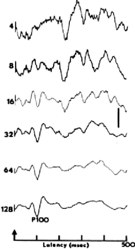
One specific class of EEG signal is the evoked potential (EP). The EP is essentially the neural response to some kind of sensory stimulus. EPs have become a large area of study as scientists and researches seek to identify and better illustrate how the brain processes information [10]. However, due to the noisiness of the EEG signal, the identification and visualization of EPs is not trivial. Oftentimes, the stimulus will be presented many times to the same human subject and EEG will be recorded. To eliminate noise, the stimulus-locked responses are then averaged (see Figure 1.2 on pg 4). This is called signal averaging and the result is a waveform that represents the EP.

Figure 1.1: International 10-20 system montage. Figure from [9].

1.2

Steady-state visual evoked potential

Visual evoked potentials (VEPs) are the neural responses of the visual sys-tem. Generally, transient VEPs are known to be evoked by sudden changes in the input signal [12].

The steady-state variety of VEPs was discovered by Regan in 1966 [13]. He experimented with using long stimulus trains of modulated light. A stable VEP was found and extracted by averaging over multiple trials. This stable response was called the steady-state visual evoked potential (SSVEP). Figure 1.3 (on pg 5) shows the main differences between VEPs and SSVEPs.

In the SSVEP, the stable response entrains to the visual stimulus which results in peaks in the frequency spectrum of the response located at the fundamental frequency and harmonics of the stimulus. On a high level, when one is presented with a flickering visual stimulus of frequency f, then the frequency spectrum of one’s brain signal will also show a peak at the same frequency f.

The SSVEP is typically recorded by electroencephalography (EEG) be-cause good time-resolution is necessary to resolve the frequency response. The EEG recording electrodes are generally placed on the back of the head because the SSVEP is thought to be generated from the occipital areas of the cortex [14].

Figure 1.2: This figure demonstrates how signal averaging cancels the noise and reveals the true evoked potential signal. The stimulus is presented at the time indicated by the arrow and numbers on the left indicate how many signals were averaged to produce the corresponding output [11].

One additional key finding is that the amplitude of the response has been found to be modulated by attention [15, 16]. That is, focusing on a stimulus causes a significant increase in the amplitude of the response peak. Thus, given two flickering stimuli (S1 flickering at f1 and S2 flickering at f2) that

are relatively close in space (thus, presented simultaneously to the subject), if a subject focused onS1, then even though the EEG spectrum of the subject

would show peaks at both f1 and f2, the peak at f1 would be significantly

larger.

Each of the properties of the SSVEP response described in the previous paragraphs is important for the application of SSVEPs to brain-computer interfaces (BCIs).

Figure 1.3: This figure demonstrates the main difference between VEPs and SSVEPs [14]. The upper section shows the VEP response to a single

stimulation. The center section shows the SSVEP response to a series of visual stimulations. The lower-left section shows the spectrum of a VEP response which has no distinct spectrum. The lower-right section shows the spectrum of an SSVEP response which has distinct peaks corresponding to the frequency of stimulation and its harmonics.

1.3

Brain-computer interfaces

In his review paper, Vialatte states that “BCIs aim to create a direct and non-muscular communication and control channel between the human brain and a computer. BCI systems need to respond relatively quickly to commands. Therefore almost all BCI systems use electroencephalographic (EEG) record-ings as the input signals” [14].

For SSVEP-based BCIs (SSVEP-BCIs), the basic idea is to encode user commands in lights that flicker at different frequencies. Users then select a command by focusing their attention on the flickering light corresponding to their desired command. The EEG data is then analyzed by the system to infer which stimulus (and thereby which command) the user was focusing on and wanted to select.

mea-sure called information transfer rate (ITR).

IT R=s

log₂(N) +plog₂(p) + (1−p) log₂

1−p N −1

(1.1) whereN is the number of available commands,sis the number of commands performed per minute, and p is the probability that a command is decoded correctly. ITR is measured in units of bits per minute [14].

Non-SSVEP-based BCIs can typically reach an ITR of 10-25 bits/min [14]; however, SSVEP-BCIs can achieve rates of at least 50 bit/min [17]. For this reason, SSVEP is one of the preferred BCI input modalities.

SSVEP-BCIs have been in development since the late 1970s [18]. However, despite this length of time, the fundamental characteristics of SSVEPs are still not understood. In his review paper, Vialatte’s final remarks describe how experimental design and paradigms are critical for developing efficient SSVEP-BCIs. He states that “unless a better understanding of the under-lying mechanisms of SSVEPs is obtained, experimental design will not be significantly improved” [14]. He calls for more basic research on the effects of experimental parameters: size of the stimulus, distance to the stimulus, brightness, etc.

This study seeks to respond to this call by investigating the effects of stimulus intensity (brightness) on the SSVEP response.

The remainder of this thesis will be organized into four chapters. Chapter 2 will contain a literature review to present the results of related works and to motivate the research of this study. Chapter 3 will describe the experiment and the analysis methods in detail. Chapter 4 will present the results, and finally, Chapter 5 will synthesize the results and present some final thoughts.

CHAPTER 2

LITERATURE REVIEW

This chapter contains an overview of the methods and results of works related to the proposed study of investigating the effect of stimulus intensity on the SSVEP response. Additionally, the relevance of the related works will also be discussed.

2.1

Stimulus contrast vs. VEP amplitude

This section discusses the paper by Campbell and Kulikowski from 1972 [19]. This paper was published to carefully verify the fit of a regression line proposed in [20]. This regression line was described as

V =Klog(C/C0) for C/C0 >1 (2.1)

where V was the voltage generated, C was the contrast of the grating used to elicit the potential, C0 was the theoretical contrast at which zero voltage

is generated, and K was a proportionality constant. Understanding such a regression line would allow for predicting the psychophysical contrast thresh-old.

2.1.1

Methods

A vertical grating was used as the stimulator. A vertical grating is a device made of vertical bars where each bar can be independently varied in intensity. The contrast of the grating was controlled by a logarithmic step-attenuator and the average luminance (light intensity) emitted by the device was main-tained to 50 cd/m2_{. The grating was presented on a circular screen to one}

For recording, one electrode was placed 2.5 cm above the inion, another was placed 2.5 cm to the right of it, and a ground electrode was placed on the forehead. The signals were differentially amplified and low and high pass filters were applied to have a pass-band of 8 to 25 Hz.

2.1.2

Results

The authors found that the evoked potential amplitude increased linearly with the log of the contrast level (see Figure 2.1). It was noted that at

Figure 2.1: Log-linear response. Figure from [19].

low contrasts (close to the threshold), the data seemed to deviate from the proposed logarithmic function.

To test if there was an effect related to the percentage of time that the grating was seen near the contrast threshold, the subject was given a switch to indicate when the stimulus was visible.

line corresponded with the contrast at which the grating was seen 50% of the time (see Figure 2.2).

Figure 2.2: The C0 intercept corresponds with the contrast at which the

grating was seen 50% of the time. Figure from [19].

2.1.3

Relevance to current study

Campbell and Kulikowski is an older study that used gratings to elicit a visual evoked response, but the repetitive nature of the stimulation points towards the SSVEP response. Moreover, this study presents an explicit regression line for estimating the amplitude of the response as a function of contrast.

Stimulation contrast is a measure that is very close to stimulation intensity. The primary difference is that contrast accounts for the difference between the light emitted in different states. Intensity refers to the total amount of light emitted.

This result (the regression line) is one that will be revisited later in the analysis of the results of the current study.

In the context of BCIs, though, Campbell and Kulikowski used a hardware system (e.g. gratings) that is not easily accessible to modern BCI developers.

It would be worthwhile to consider the effects of intensity (and contrast) using modern equipment and analysis tools.

2.2

Ambient lighting and stimulus contrast vs. BCI

performance

This section discusses the paper by Bieger, Molina, and Zhu from 2010 [21]. SSVEP-BCI performance is often affected (sometimes significantly) by stim-ulus properties (e.g. stimulation frequency). On the other hand, since these systems may be used for long periods of time, comfort is another important factor to consider when developing such systems. This study seeks to in-vestigate the effects of stimulation properties on performance and comfort in SSVEP-BCI systems. The stimulus properties that are considered are: the stimulation device, environmental illumination, contrast, color, spatial frequency, and size. For the purpose of this literature review, the discus-sion of methods and results will focus on the environmental illumination and contrast because these properties are directly related to stimulus intensity.

Environmental illumination and contrast are closely related properties. Contrast is typically defined as

C = Imax−Imin

Imax+Imin

×100% (2.2)

whereImax andImin are the maximum and minimum intensities respectively. It follows that changes in the environmental illumination affect bothImaxand

Iminwhich affects the value of the ratio. It should also be obvious that greater contrasts can be achieved in darker (lower illumination) environments.

2.2.1

Methods

Ten people (7 male, 3 female) participated in the study, but only 6 partici-pated in each of the experiments. The participants were between 24 and 32 years of age and had normal or corrected-to-normal vision. They were seated comfortably approximately 70 cm from the stimulation devices. Electrodes were placed in 32 positions over the scalp according to the international 10-20 system, but only the 8 channels covering the occipital region were

re-referenced to channel Cz and used by the BCI system. The frequencies that each subject used were selected in a 3 minute long frequency selection pro-cess for selecting the frequencies that worked best. Each experiment was also preceded by a 3 minute long calibration phase.

The experiments in question here were carried out using an LCD monitor with a refresh rate of 75 Hz and 6 cm by 6 cm flickering stimuli.

It was not specifically specified how the experimenters adjusted the en-vironmental illumination or the contrast level of the stimuli. To evaluate comfort, users completed an empirically designed questionnaire before the experiments. On the questionnaire, they indicated how pleasant, tiring, and annoying the conditions were and how long they could look at them on 7-point scales. The questionnaire responses were aggregated into a single com-fort score where a 1 indicated low comcom-fort and a 7 indicated high comcom-fort.

For each experiment, the users had to move an avatar along a curvy cor-ridor to a goal space using the SSVEP-BCI system. The users moved the avatar by focusing their attention on the flickering stimuli associated with the intended direction. Correct moves were accompanied by a green screen flash and a high-pitched tone and incorrect moves were followed by a red flash and a low-pitched tone. Each move was also followed by a one second period of inactivity to provide the user with enough time to reorient their focus and for the previous SSVEP response to diminish.

For classification, the BCI system estimated the power in the EEG signal at the frequencies (and harmonics) associated with the possible targets. The signal was first preprocessed with a 50 Hz IIR notching comb filter to remove power line interference. Then the power for the targets was estimated by applying a maximum contrast spatial filter for the first 4 harmonics of each target frequency. The resulting harmonics were then peak filtered, squared, and averaged over the last second. The sum of these powers for each target was then used for classification. A class was selected whenever the power for exactly one target exceeded the associated threshold. The frequencies, spatial filters, and thresholds are predetermined during the frequency selection and calibration phases of each of the experiments.

2.2.2

Results

The results of this experiment indicated that BCI performance was positively correlated with contrast. That is, users performed better with the BCI sys-tem when the contrast was higher. Bright backgrounds were also generally judged as uncomfortable. For environmental illumination, the darker envi-ronment was shown to have better performance, but subjects mentioned that they preferred the more natural condition where the lights were on.

2.2.3

Relevance to current study

The results of this study seem to indicate that ambient lighting and stim-ulation contrast do have some effect on the response–enough that the BCI performance is affected. This further supports the statements of [14] that understanding how experimental parameters affect the SSVEP response is critical for optimizing SSVEP-BCI systems. These results also fall in line with the result of [19]. Campbell found that high contrast levels will evoke larger VEPs which are easier to classify in SSVEP-BCIs.

With respect to the current study on the effects of stimulus intensity, these results are generally supportive of the hypothesis that the SSVEP response is positively correlated with stimulus intensity. It is unclear if the contrast experiments controlled for maintaining the amount of light emitted at a con-stant level like [19]. It is likely that at a concon-stant ambient light level, in-creasing contrast also increased the stimulus intensity in these experiments. Taking this and the results together, it could be that BCI performance is positively correlated with stimulus intensity. This would suggest that the strength of the SSVEP response is positively correlated with stimulus in-tensity because stronger responses are easier to classify and lead to better performance.

2.3

Stimulus size vs. SSVEP response

This section discusses the publication of Duszyk et al. in 2014, [22]. Once again, in this study, the authors investigated the effect of different stimulus properties on the SSVEP response for BCI systems. The authors’ aim was

to design optimal stimuli for use in assistive BCI applications for individuals with neuromuscular disorders. Five different stimuli parameters were tested: size, inter-stimulus distance, color, shape, and the presence of a fixation point. This literature review will focus on the methods and results relevant to testing the effect of stimulus size on the SSVEP response.

2.3.1

Methods

Two separate experiments were performed in this study. The first experi-ment tested the 5 stimulus parameters that could potentially influence the magnitude of the response. Based on the results of the first experiment, the second experiment further investigated 3 of the stimulus parameters that showed an effect.

In the first experiment, 5 young adults (µage = 25.8, σage = 1.79) of both sexes participated. In the second experiment 20 subjects (µage = 27.2, σage = 3.3) participated in the study. All subjects were screened for photogenic epilepsy, neurological and psychiatric disorders, and use of med-ications known to adversely affect EEG recording. All subjects also signed off on written consent forms.

During the experiment, subjects sat in a darkened room, one meter away from the stimulus display. Two desk lamps acted as the only light sources in the room. Four stimuli were presented simultaneously and subjects were given an auditory instruction to focus on one of the 4 stimuli. Each stimulus flickered at a different frequency (14, 17, 25, and 30 Hz). Stimuli were pre-sented with 4 different side lengths (41, 102, 170, and 255 pixels). In the first experiment, all four side lengths were presented. In the second experiment, only the latter 2 side lengths were presented. During a stimulation cycle, the stimuli flickered for 4 seconds and were completely black for a 6 second rest period.

Stimuli were presented via a hybrid LCD/LED device. This device con-sisted of an array of LEDs underlaid below and LCD screen. The LEDs highlighted precisely determined areas of the screen. Each of the four stimu-lation areas displayed on the LCD was highlighted by a group of LEDs. This allowed the experimenters to fully control the stimulus appearance, while also avoiding problems such as monitor refresh rate.

EEG recording was performed with a sampling rate of 1,024 Hz. Twenty electrodes were used with 19 being placed according to the 10-20 interna-tional system and the 20th electrode placed at FCz. The averaged signal from the mastoids (M1 and M2) was used as the reference signal and the ground electrode was placed on the chest near the breastbone. All electrode impedances were kept below 5 kΩ.

For analysis, 7 channels were used: O1, O2, Pz, P3, P4, P7, and P8. The signals were down-sampled to 128 Hz. Then from the specified channels, two classes of segments were extracted: a 4 second epoch of data measured during visual stimulation, and a 4 second long epoch of data measured before the on-set of stimulation. Data was then band-pass filtered with a pass-band width of 2 Hz for each of the frequencies. The pre-stimulus and during-stimulus epochs were converted to power spectra and then the SSVEP strength was computed as the Event Related Spectral Perturbation (ESRP) [23]. ESRP is a measure of the relative change in SSVEP power. This is a useful measure because it is known that the spectral power of EEG decreases as frequency increases. This means that the response to high-frequency SSVEP has a lower absolute power than the response to low-frequency stimulation. ESRP is defined as ESRPf = P + f −P − f P_f− (2.3)

where for a given frequency f, P_f+ is the average power during stimulation and P_f− is the average power before stimulation.

2.3.2

Results

In the first experiment, a strong, positive, linear effect was observed for SSVEP power with an increase in stimulus size. In the second experiment, the results of the first experiment were further confirmed. Larger stimuli sizes consistently produced stronger SSVEP responses (as measured by ERSP). The results are summarized in Figure 2.3. The results of the first experiment are shown in Figure 2.3a and those of the second experiment are shown in Figure 2.3b.

(a) The results of the first experiment considering stimulus size. There is a strong linear effect of stimulus size on the strength of the SSVEP response.

(b) The results of the second experiment considering stimulus size. The effect observed in the first experiment (see Figure 2.3a) was further confirmed.

Figure 2.3: Experimental results for stimulus size studies. Figures from [22].

2.3.3

Relevance to current study

Similarly to [21], which was discussed in Section 2.2, these results are also indirectly related to the current study of stimulus intensity. Increasing the size of the stimulus will naturally also increase the amount of light emitted, thereby increasing the stimulus intensity. Similarly to before, the result ob-served in this study would also imply that SSVEP power increases as stimulus intensity increases. This result also means that an investigation into stimulus intensity should control for stimulus size.

2.4

Viewing distance vs. SSVEP response

This section discusses the paper by Wu and Lakany in 2013, [24]. At present, most SSVEP-BCI systems require the stimulator to remain close to the user which limits the portability of these systems. In this study, the authors aim to develop a portable SSVEP-BCI system that can adapt to changes in the distance between users and the flickering visual stimuli. In order to develop a more portable system, the authors investigated the impact of the distance between the user and the stimulator (viewing distance) on the SSVEP response.

2.4.1

Methods

Two subjects (1 male, 1 female) participated in this study. They were seated comfortably in a dim room during the experiment. The EEG recording used a 128-channel EEG cap using the 10-20 international system. Eleven channels over the visual cortex were used for data collection: POz, 124, 125, O1, Oz, O2, 127, 128, O9, Iz, and O10. Cz was chosen as the ground and Fz was used as the reference channel. Electrode impedances were kept under 5 kΩ. EEG data was sampled at 2,000 Hz.

The stimulator used one red LED (7,100 mcd for higher intensity, 2,525 mcd for lower intensity). The LED was driven by a microcontroller that generated a square wave of 12, 13, 14, or 15 Hz with a duty cycle of 50%. One of the frequencies was chosen for each run of the experiment and the same frequency was used throughout the entire run.

The experiment consisted of 16 runs which used different combinations of the 4 LED intensities and the 4 viewing distances, 60, 150, 250, and 350 cm. The LED intensities are not reported in the paper; however, the different intensities were achieved by altering the value of the serial resistor with the LED and/or using a different LED. Each run consisted of 20 trials. Each trial included a resting phase and an attending phase. EEG was recorded while the subject was attending to the stimuli. The resting phase lasted for 5 to 6 seconds (the exact duration was randomly chosen), during which the LED was off. During the attending phase, which lasted for 5 seconds, the LED was flickering at the selected frequency.

extracted consisting of EEG data from 1 second before stimulus onset to 4 seconds after stimulus onset. Off-line analysis of the EEG data consisted of visualization and classification. Visualization was performed using the fast Fourier transform (FFT), and a number of other methods: event-related spectral perturbation (ERSP, described previously), inter-trials coherence and stimulus-locked inter-trace correlation. These other methods will not be further discussed in this literature review. Classification was performed using canonical correlation analysis (CCA).

For more details on the FFT and CCA which are used in the current study, please see Appendix A.

2.4.2

Results

Figure 2.4a (on pg 19) clearly shows that SSVEP power decreases signif-icantly (p = 7.38× 10−8) as viewing distance increases. However, when intensity compensation is added (Figure 2.4b), the SSVEP power remains relatively high even at greater distances such as 250 cm. In this study, in-tensity compensation is not explicitly described, but it is said that the LED intensities used at 150, 250, and 350 cm are greater than that used at 60 cm. For classification results, the authors presented three tables: the effect of viewing distance without intensity compensation, the effect of viewing distance with intensity compensation, and the effect of different intensities.

For the effect of viewing distance without intensity compensation, they found that the classification rate for the 12 Hz condition was not signifi-cantly affected by viewing distance. However, it is notable that classification results seem to be consistently biased towards 12 Hz. Excluding the 12 Hz classification rate, for distances greater than 150 cm, the average classifica-tion rate is only 20%.

With intensity compensation, the average classification rate of the longer viewing distances increases significantly to 75%.

For the interaction between intensity and the classification rate, classifica-tion accuracy tended to increase as the intensity was increased.

2.4.3

Relevance to current study

The addition of intensity compensation significantly increases the SSVEP power even at greater viewing distances. This result clearly implies that stimulus intensity has a significant effect on the power of the SSVEP response. Given the four data points provided in Figure 2.4a, a linear model can be fit to the data. The viewing distances (60, 150, 250, and 350 cm) can be converted to relative intensities with

Iri = 1 di d60 2 (2.4)

wherediis one of the distances,Iriis the corresponding relative intensity, and

d60 is 60 cm. This formula is derived from the well-known inverse law which

describes how light intensity is proportional to the inverse squared distance to the light source. Doing this results in the following relation (Figure 2.5 on pg 20). With a p-value of 0.02, it can be seen that there is a significant non-zero relationship between intensity and the FFT power. Moreover, with an R2 _{value of 0.96, the linear model appears to be a good fit for the data.}

It is important to recall that this is still a fit to only four points of data from a single subject. This being the case, the fit is subject to noise and may not be reflective of the true relationship.

With respect to the current study, these results implicate another potential relationship that one would expect to observe (a linear relationship between intensity and SSVEP strength) from a more rigorous investigation of the effect of stimulus intensity on the SSVEP response.

(a) FFT power without intensity compensation

(b) FFT power with intensity compensation

Figure 2.4: Plots showing FFT power as a function of distance. Figures from [24].

Figure 2.5: FFT power as a function of relative (to the 60 cm intensity) intensity. The p-value indicates that the slope of the linear fit is

significantly different than 0 and the R2 value indicates that for the four data points, the linear model is an excellent fit.

CHAPTER 3

METHODS

This chapter presents the methods used in the experiment in greater detail. The experimental protocol will be divided into 6 main sections: subjects, stimulation, physical setup, EEG recording, experimental timing, and data analysis.

3.1

Subjects

10 healthy subjects (2 female, 8 male) participated in the study. All subjects had normal or corrected-to-normal vision. All subjects signed consent forms to indicate their voluntary participation. This human-subject experiment was approved by the Institutional Review Board at the University of Illinois at Urbana-Champaign.

3.2

Stimulation

Light stimulation was delivered using a white light-emitting diode (LED) panel measuring 3 cm by 3 cm. The panel was an 8 pixel by 8 pixel, 250 mcd, LED matrix. The stimulator was driven and powered by a field-programmable gate array (FPGA).

Stimulation consisted of flickering the LED panel at a frequency of 7 Hz. Flickering involved alternating between on and off states for the entire LED matrix simultaneously. This delivered square-wave stimulation to the sub-ject. The FPGA had a 50 MHz clock which allowed for a very precise stim-ulation.

Precise stimulation is very important because the strength of the SSVEP response is affected by imprecise stimulation. It has been shown that LED stimulators produce SSVEP responses that are significantly stronger than

those produced by LCD and CRT stimulators [25]. The spectra of LCD and CRT stimulations are far noisier than that of LED stimulation. This is likely because LEDs have far shorter rising times than LCDs and are not limited by the low refreshing frequencies of LCD and CRT monitors so they can better approximate square-waves.

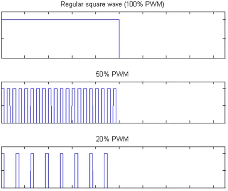
To vary the intensity of the stimulation, pulse width modulation (PWM) was implemented on the FPGA. PWM in this application allowed for fine-grained control of the total power delivered by the LED panel.

PWM was accomplished by rapidly modulating the total amount of time that the panel was on (see Figure 3.1). For example, to achieve 50% of the max intensity with a PWM modulation frequency,fP W M, during the on state of the 7 Hz stimulation, the panel is turned on for one PWM cycle, 1/fP W M, and then off for the next PWM cycle. This is repeated for the entire on state, causing the panel to only be on for half of the duration of the on state, thus 50%. As another example, to achieve 20% of the max intensity with the same

fP W M, the panel is turned on for one PWM cycle, and then off for the next four PWM cycles. If the PWM modulation frequency, fP W M, is chosen to be sufficiently high, then there will be no aliasing effects on the stimulation signal and the stimulus intensity can be very precisely adjusted.

The PWM modulation frequency used for this experiment was 2 MHz. PWM modulation levels of 0 (the panel remained off as a control case), 10, 20, 30, 40, 50, 60, 70, 80, 90, and 100 percent were used.

3.3

Physical setup

The stimulation device was placed 45 cm directly in front of subjects. Their heads were held in position with a chin rest. Ambient lighting for all of the experiments was maintained at around 5 Lux which is the normal, dim room, lighting condition used in BCI experiments.

3.4

EEG recording

EEG recording was taken from 6 channels according to the international 10-20 system: PO3, POZ, PO4, O1, OZ, and O2. The channels were referenced

Figure 3.1: A simplified example for demonstrating how pulse width

modulation works. At a 100% PWM modulation level, the output is simply a square wave. Notice that at a 50% and 20% PWM level, the signal goes high and low rapidly according to a predetermined fP W M.

to the top of the head and grounded to the right ear. Signals were sampled at 512 Hz and all electrode impedances were below 10 kΩ during recording.

3.5

Experimental timing

Each experiment consisted of 8 blocks of trials and was about 30 minutes in duration. Subjects were allowed to rest for about 1 minute between blocks. In order to keep subjects engaged, they were told riddles and jokes in this break time. Each block consisted of 11 trials where each of the PWM modulation levels was presented once per block in a random order. Each trial consisted of 10 seconds of stimulation. Subjects were asked to focus on the blinking light during stimulation. The interstimulus interval, or length of time between trials, was uniformly selected between 5.025 and 5.5 seconds.

3.6

Data analysis

The EEG data was analyzed using the FFT and CCA (for more details, see Appendix A.1 and A.2).

In the FFT analysis (see Algorithm 1), all of the EEG data was analyzed by first band-pass filtering between 1 and 25 Hz. This eliminated high-frequency noise from the data (such as 60 Hz power line noise). The mean and linear trends were then removed from the data. Finally, a 1024-point FFT was computed. Post-processing included averaging over channels for each class of each subject. For more information on motivating many of these decisions, see Appendix A.3.

input : D, EEG data of sizeB ×T ×C×S

output: F, Transformed EEG data of size B×T ×C×N

for b←1 to B do for t←1 to T do for c←1 to C do X ← D[b, t, c] X ← filter(X,[1,25]) X ← detrend(X) F[b, t, c]← FFT(X, N) end end end

Algorithm 1: FFT analysis algorithm for a given subject with B blocks of data, T trials of data per block, C channels of data per trial, S samples of data per channel, and a N-point FFT

The CCA analysis algorithm is described in Algorithm 2. Since CCA can leverage correlated information between channels, CCA coefficients are not computed channel by channel. CCA does, however, have more parameters such as frequency resolution, window length, and the amount of overlap and harmonics to use.

In this study, the frequencies considered in CCA analysis were 5 to 15 Hz in steps of 0.1 Hz. The entire 10 second window of stimulation data was used as the window length (therefore there was also no overlap) and 2 harmonics were used.

After the data from each subject was analyzed using the FFT and CCA, subject data was combined to perform group analysis.

input : D, EEG data of sizeB ×T ×C×S

output: C, CCA coefficients of size B×T ×F ×W

for b←1 to B do for t←1 to T do X ← D[b, t] C[b, t]← CCA(X,Θ) end end

Algorithm 2:CCA analysis algorithm for a given subject withB blocks of data, T trials of data per block, C channels of data per trial, S samples of data per channel,F frequency bins,W time windows, and CCA parameters, Θ.

For group analysis, the FFT amplitudes and CCA coefficients correspond-ing to the first (7 Hz) and second (14 Hz) harmonics of the SSVEP response were extracted. The second harmonic was also included in the analysis be-cause some BCI classification algorithms (such as CCA) can take advantage of harmonic information.

In the case of FFT, since different subjects have different noise floors and signal strengths, data was normalized for each individual subject before av-eraging across subjects. For a 0% PWM response of F0, the X% PWM

response (FX) was normalized with

FXnorm=

FX −F0

F0

(3.1) For CCA, since the computed correlation values are already normalized, CCA coefficients were simply averaged across subjects.

Lastly, a linear model was fit to the FFT and CCA data to model how the FFT amplitudes and CCA coefficients were affected by changes in intensity (or PWM level in this experiment).

CHAPTER 4

RESULTS

The results of this study are described in this chapter. The first section will discuss subject-by-subject (individual) results. The second section will present group results. Each section will begin by describing the primary plots associated with the section. The results will then be compared to other results observed in the literature in a final section.

4.1

Individual results

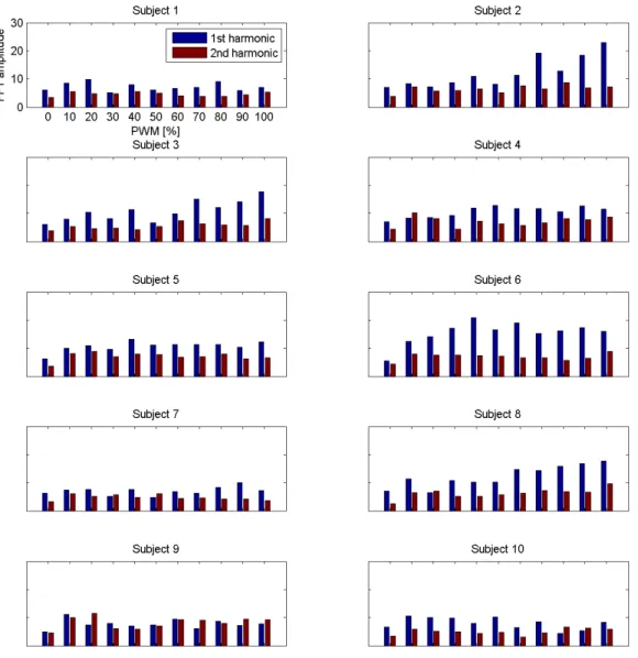
Figures 4.1 and 4.2 (on pg 27 and pg 28) show individual responses as a function of the PWM level. The first harmonic responses correspond with the FFT amplitudes and CCA coefficients centered at 7 Hz. The second harmonic responses correspond with 14 Hz. All subplots are on the same scale.

A great amount of variability in the responses between subjects is apparent. Inter-subject variability in EEG data is known to be due to different cortical geometries between people [26]. The noise inherent in the EEG signal also contributes to the variance. Because of this, data between subjects will have different noise floors and response amplitudes. To account for these differences, careful normalization is necessary before combining subject data for group analysis.

Despite the variance, a some trends (correlation between a 10% PWM level and a 100% PWM level) can still be observed (in the first harmonic response) on a subject level. Table 4.1 shows the correlation coefficients R computed for both FFT and CCA data between the 10% PWM level and the 100% PWM level.

In the FFT responses, positive correlations (R >0.5) can be observed for Subjects 2, 3, 4, and 8). Slight positive correlations (0.1 < R < 0.5) are

Figure 4.1: Individual FFT responses for the first and second harmonics of each subject.

Table 4.1: Correlation coefficients, R, by subject.

FFT CCA

Subject R Subject R Subject R Subject R

1 -0.274 6 0.263 1∗ -0.780 6∗ 0.742

2∗ 0.865 7 0.351 2∗ 0.921 7 -0.104

3∗ 0.780 8∗ 0.882 3∗ 0.784 8∗ 0.920

4∗ 0.706 9 -0.359 4∗ 0.913 9 -0.536

5 0.362 10∗ -0.710 5 0.499 10 -0.525

An asterisk by the subject number indicates a significant correlation (p < 0.05).

Figure 4.2: Individual CCA responses for the first and second harmonics of each subject.

seen for Subjects 5, 6, and 7. Negative correlations (R <0) are observed for Subjects 1, 9, and 10.

When considering the CCA responses, Subjects 2, 3, 4, 6, and 8 show pos-itive correlations, Subject 5 shows a slight pospos-itive correlation, and Subjects 1, 7, 9, and 10 show negative correlations.

It is worthwhile to mention that Subject 2 displayed the most prominent trend in the subject’s first harmonic response. In particular, when consider-ing the individual CCA results of Subject 2, for a 10% PWM level, the CCA coefficient is 0.192. However, at a 100% PWM level, the CCA coefficient is 0.498. CCA coefficients are restricted to fall within the range of 0 and 1, so this difference (0.306) may be considered large. Such a difference could

impact the performance of the subject in SSVEP-BCIs that use CCA for classification. Table 4.2 shows the change in CCA coefficients (between a 0% PWM level and a 100% PWM level) for each of the subjects.

Table 4.2: The difference in CCA coefficients between the 10% PWM level and the 100% PWM level for each subject.

Subject 10% 100% % change Subject 10% 100% % change

1 0.355 0.301 -15.2% 6 0.338 0.461 36.4% 2 0.192 0.498 159.4% 7 0.457 0.449 -1.8% 3 0.281 0.523 86.1% 8 0.630 0.779 23.7% 4 0.413 0.617 49.4% 9 0.417 0.380 -8.9% 5 0.506 0.560 10.7% 10 0.341 0.312 -8.5%

4.2

Group results

Figures 4.3a and 4.3b show group-level responses as a function of PWM level. Recall that in the CCA results, the subject data was normalized according to Equation 3.1 before combining together into group results.

In each figure, the upper 2 panels show the first harmonic (7 Hz) responses. The lower 2 panels show the second harmonic (14 Hz) responses.

The marks in the left panels show individual responses across subjects and blocks. Since each of the 10 subjects participated in 8 blocks of trials, there are 80 observations for each of the PWM levels. Outlying points are clearly visible near the top of the FFT plots. These outliers are not evident in the CCA plots. This is likely because CCA does a better job of normalizing the data across subjects.

The right panels show the average overall response and the linear model that was fit to the data. Each error bar represents a single standard deviation for the corresponding PWM level. Crosses denote the mean response value for each PWM level across all blocks and all subjects. Finally, the red line shows the linear model that was calculated from the data. Above the panels on the right side are p-values and correlation coefficients, R. The p-values are produced by the F-test for regression and indicate the significance of R

and the slope of the fitted lines.

Note that the slopes are all relatively shallow, but the p-values are sig-nificant (p < 0.05) for all of the slopes except the second harmonic, FFT

(a) Group level FFT responses for the first and second harmonic amplitudes.

(b) Group level CCA responses for the first and second harmonic coefficients.

Figure 4.3: Group level responses. responses.

The remainder of the discussion of the results will be separated by har-monic: first, and then second.

4.2.1

First harmonic responses

For the first harmonic responses, the linear model almost certainly has a non-zero, positive slope (pF F T = 4.629×10−6, pCCA = 9.122×10−7). This also indicates that the first harmonic amplitude of the SSVEP response is significantly correlated with stimulus intensity.

The R2 values from the line fit are very small with R2_{F F T} = 2.597×10−2 and R2

CCA = 2.977×10

−2_{. Normally, R}2 _{values that are this small would}

suggest that the linear model is not a good fit for the data, or that it does not describe most of the variance in the data. However a plot of the residuals (Figure 4.4) does not appear to reveal any trends (non-randomness) that would implicate a different model.

If any trends were discernible in the residual plot, then it would suggest that there is information in the data that is not being described by the model. Thus, for a good fit, residual plots should look randomly distributed.

After inspection, the residuals do appear randomly distributed. Further-more, the p-value given in Figure 4.4 (p ≈ 1.000) confirms that the line fit to the residual data does indeed have 0 slope. In this case, the variance of the data is most likely due to inter-subject variability and noise in the EEG signal.

To test if the linear effect was being dominated by a single outlying subject, the subjects were individually omitted from the group analysis to test if the effect became insignificant. The results in Table 4.3 show that the observed significant effect is group behavior.

Table 4.3: The p-values corresponding to the linear model fitted to group FFT data after omitting the given subject.

Subject omitted p-value Subject omitted p-value 1 7.351×10−7 6 1.802×10−7 2 4.999×10−3 _{7 6.119×10}−6

3 5.573×10−4 _{8 6.671×10}−4

4 2.340×10−5 9 3.804×10−7 5 4.587×10−6 _{10 4.984×10}−8

(a) Residuals from the best-fit line to the first harmonic, FFT amplitudes.

(b) Residuals from the best-fit line to the first harmonic, CCA coefficients.

Figure 4.4: Residual plots for the 1st harmonic linear model.

4.2.2

Second harmonic responses

For the second harmonic, it is unclear if there is a linear effect or not. With a p-value of 4.088×10−1_{, stimulus intensity does not seem to have an}

ef-fect on the FFT response. However, when the SSVEP response is analyzed with CCA, a p-value of 9.391×10−6 is observed indicating that the relation between stimulus intensity and the strength of the response has a non-zero slope. These differences might be due to noise or differences between the FFT and CCA analysis methods. At this stage, it is difficult to conclude

whether or not there is an effect in the second harmonic.

For the CCA linear model, analysis of the R2 _{values and residuals, as}

before, revealed the same as for the 1st harmonic responses. R2 _{values are}

low, but the residual plots don’t seem to show any correlated behavior that would suggest a different model.

4.3

Relations to the literature

The results observed in this study are generally in line with those described in previous literature.

As stated before, the studies of [21, 22, 24] indirectly found that the strength of the SSVEP response increased as stimulus intensity increased. In particular, the linear result (Figure 2.5) derived from Wu’s data [24] was also observed in the results of this study. The slope observed in the current data is not as pronounced as that of Wu, but it is unclear how the stimulus intensities compare between the studies.

Campbell and Kulikowski [19] provided an explicit relationship (repeated here).

V =Klog(C/C0) for C/C0 >1 (4.1)

This model is in terms of contrast rather than intensity, but since the current study was performed with a set ambient lighting condition, the intensity is equivalent (by a factor) to contrast.

Equation 4.1 describes a logarithmic relationship which differs from the linear relationship observed with the data in this study. It is worth men-tioning that the intensities (contrasts) used in this study were closely spaced and nowhere near the contrast threshold (subjects could clearly see the LED panel flicker) as many of the contrasts used by Campbell and Kulikowski. Therefore it is possible that the intensities used in the current study fall within a linear region of the logarithmic function.

For instance, given f(x) = logx, df_dx(x) = _x1. Since lim x→∞

1

x = 0, it can be said that logx becomes linear as x goes to infinity. On the other hand, given a range, or window, of x values andf(x) = logx, the definition of the derivative states that f(x) will approximate a linear function as the window of x becomes very small.

CHAPTER 5

CONCLUSION

Previous research has implied a relationship between stimulation intensity and the strength of the SSVEP response. The results of this study are an additional step to further support that the SSVEP amplitude is positively correlated with stimulation intensity.

This study was performed with normal BCI conditions and found that for the range of stimulus intensities tested, there is a significant correlation (RF F T = 0.161, pF F T = 4.629×10−6;RCCA = 0.173, pF F T = 9.122×10−7) between stimulus intensity and the amplitude of the SSVEP response. The CCA results are important because CCA is one of the most popular SSVEP classifiers. For one subject (Subject 2), a difference of 0.30 (≈160% increase) was observed between the CCA correlation coefficients stimulated at the 10% PWM condition and 100% PWM condition. CCA correlation coefficients are limited to fall within a range of 0 and 1 so a difference of this magnitude may have significant effects on the BCI user performance for this subject. An effect of this magnitude was not observed for all of the subjects, but is worth further investigation.

Understanding the SSVEP response is important so that researchers can properly design their experiments to optimize SSVEP-BCI systems [14]. Within this context, this research, as well as other literature, has observed significant correlations in the strength of the SSVEP response as a function of stimulation intensity. Furthermore, this study has identified stimulation intensity as one experimental parameter that may have a significant impact on the user performance with SSVEP-BCI systems. However, more research is necessary to fully understand the extent of this impact. For instance, fur-ther investigation is necessary to understand why some subjects show large effects. Also this study does not dissociate the effects of stimulus intensity and stimulus contrast. It is therefore unclear if the observed effect is dom-inated by intensity or contrast effects (or both). It would be interesting to

compare SSVEP responses generated by a low-intensity, high-contrast stim-ulation with those generated by a high-intensity, low contrast stimstim-ulation. Additionally, it would be worthwhile to consider PWM intensities between 0% and 10% to verify that the logarithmic relationship derived in [19] holds in these low-contrast conditions.

APPENDIX A

ANALYSIS METHODS

This appendix contains more detail about the analysis tools and methods relevant to this study.

A.1

Fourier transform

The Fourier transform is a method of transforming time-domain data to the frequency domain. It accomplishes this by taking advantage of the Fourier theorem which states that all signals can be decomposed into a sum of weighted sines and cosines. The Fourier transform visualizes these weights to provide a sense of the frequency content in a signal. The more prevalent a frequency in a signal, the stronger the corresponding peak in the frequency spectrum. Consider the following example with signal X.

X = sin(2π7t) + 2 sin(2π15t) + 3 sin(2π24t) (A.1) Figure A.1a shows the time-domain representation of the components of X

and the composition of X. Figure A.1b shows the frequency spectrum of the composed signalX. Notice that the relative peak amplitudes correspond with the given equation for X (Equation A.1).

The fast Fourier transform (FFT) is a particular implementation of the Fourier transform that has been optimized for computing systems efficiently compute the Fourier transform. The speed at which the FFT of a signal can be computed makes it one of the most common ways of visualizing EEG data in the frequency domain [14, 24]. Since the SSVEP achieves a steady-state response at the known stimulation frequencies, the SSVEP spectrum is a popular method of visualizing the strength of the response. That is, the strength of the SSVEP signal will correspond with the amplitude of the peaks in the spectrum.

A.2

Canonical correlation analysis

CCA is used to classify SSVEPs by investigating the relationship between two sets of variables, the EEG data and a reference set [27]. Much is known about the SSVEP signal, and this information can be leveraged to design the reference set. For instance, it is known that the SSVEP shows power at the fundamental frequency of stimulation and harmonics [14]. This being the case, a set of sines and cosines with frequency content at the fundamental frequency of stimulation and harmonics works naturally as the reference set [27]. Thus for a stimulation frequency, f, the reference set will be

Y(t) =          y1(t) y2(t) y3(t) y4(t) .. .          =          sin(2πf t) cos(2πf t) sin(4πf t) cos(4πf t) .. .          (A.2)

CCA finds a linear combination of the EEG data and the reference set of sines that maximizes the correlation between the two variables. This lin-ear combination also has the effect of computing a spatial filter across the multiple EEG channels for maximizing the SSVEP signal.

Classification is generally performed by computing CCA coefficients for each of the stimulation frequency classes and choosing a class when one of the CCA coefficients passes a threshold value. Thus, the value of the CCA coefficient is critical for classification in SSVEP-BCI systems.

A.3

Fourier analysis of steady-state potentials

A paper published by Bach and Meigen in 1999 provides insight into sug-gested methods of Fourier analysis when applied to steady state signals [28]. The authors suggest that since a great amount is known about the input and the output signals, artifacts in the output signal can be avoided by selecting analysis parameters carefully. Three of the major suggestions are accounted for in this study: (1) the analysis window should contain an integer num-ber of stimulation periods, (2) trend artifacts should be removed, and (3) smoothing window functions are not necessary and introduce artifacts.

Figure A.2, from [28], visualizes the problems that occur when a non-integer number of periods is included in the analysis window. This is due to the Fourier assumption that signals are periodic. When the tail of the signal is concatenated with the head, if the signal does not contain an integer number of periods, then a sharp point or discontinuity will be formed. Sharp points and discontinuities in the FFT are manifested as high-frequency content.

To account for this in the present study, an analysis window of 10 seconds was taken. Since the stimulation frequency was 7 Hz, a 10 second window will include 70 stimulation periods. Using this much data also allows for high frequency resolution and accurate detrending.

Figure A.3, from [28], shows the result of having trend artifacts in the data. These artifacts may come from the slow decay of large deflections caused by blinking or other motor activity. This generates additive noise in the spectrum.

This effect was accounted for in the present study by detrending the data before the FFT was computed.

Finally, Figure A.4, from [28], shows the result of applying smoothing windows to the data. Smoothing windows are generally applied in Fourier analysis when segmenting the data. However, when analyzing steady-state responses, smoothing windows are unnecessary because the data can already be segmented in such a way to eliminate those artifacts, and windowing actually introduces more artifacts by attenuating the periodic response near the edges of the window.

Smoothing windows were not applied in this study to avoid introducing this artifact.

(a)

(b)

Figure A.1: These plots show the effect of composing sinusoidal signals together and the resulting Fourier spectrum.

Figure A.2: The effect of choosing an analysis window with a non-integer number of stimulation periods.

Figure A.3: The effect of linear trends on the spectrum of a signal.

REFERENCES

[1] L. Haas, “Hans Berger (1873-1941), Richard Caton (1842-1926), and electroencephalography,” Journal of Neurology, Neurosurgery & Psy-chiatry, vol. 74, no. 1, 2003.

[2] D. Kupfer et al., “The application of EEG sleep for the differential diagnosis of affective disorders,” American Journal of Psychiatry, vol. 135, no. 1, 1978.

[3] F. Mormann et al., “Mean phase coherence as a measure for phase syn-chronization and its application to the EEG of epilepsy patients,” Phys-ica D: Nonlinear Phenomena, vol. 144, no. 3, 2000.

[4] R. Williams and K. Herrup, “The control of neuron number,” Annual Review of Neuroscience, vol. 11, no. 1, pp. 425–453, 1988.

[5] M. Teplan, “Fundamentals of EEG measurement,” Measurement Sci-ence Review, vol. 2, no. 2, pp. 1–11, 2002.

[6] P. Nunez and R. Srinivasan, Electrical Fields of the Brain: The Neuro-physics of EEG. New York, NY: Oxford University Press, 2006. [7] G. Gratton, M. Goodman-Wood, and M. Fabiani, “Comparison of

neu-ronal and hemodynamic measures of the brain response to visual stimu-lation: an optical imaging study,”Human Brain Mapping, vol. 13, no. 1, pp. 13–25, 2001.

[8] W. Tatum IV, Handbook of EEG Interpretation, 2nd ed. New York, NY: Demos Medical Publishing, 2014.

[9] G. Klem et al., “The ten-twenty electrode system of the international federation,”Electroencephalography and Clinical Neurophysiology, Suppl 52, pp. 3–6, 1999.

[10] D. Lehmann and W. Skrandies, “Spatial analysis of evoked potentials in man–a review,” Progress in Neurobiology, vol. 23, no. 3, pp. 227–250, 1984.

[11] K. Chiappa, Evoked Potentials in Clinical Medicine, 3rd ed. Philadel-phia, PA: Lippincott Williams & Wilkins, 1997.

[12] E. Courchesne, S. A. Hillyard, and R. Galambos, “Stimulus novelty, task relevance and the visual evoked potential in man,” Electroencephalogra-phy and Clinical NeuroElectroencephalogra-physiology, vol. 39, no. 2, pp. 131–143, 1975. [13] D. Regan, “Some characteristics of average steady-state and transient

responses evoked by modulated light,”Electroencephalography and Clin-ical Neurophysiology, vol. 20, no. 3, pp. 238–248, 1966.

[14] F.-B. Vialatte et al., “Steady-state visually evoked potentials: focus on essential paradigms and future perspectives,” Progress in Neurobiology, vol. 90, no. 4, pp. 418–438, 2010.

[15] S. T. Morgan, J. C. Hansen, and S. A. Hillyard, “Selective attention to stimulus location modulates the steady-state visual evoked potential.”

Proceedings of the National Academy of Sciences, vol. 93, no. 10, pp. 4770–4774, 1996.

[16] M. M¨uller, W. Teder-S¨alej¨arvi, and S. Hillyard, “The time course of cortical facilitation during cued shifts of spatial attention,”Nature Neu-roscience, vol. 1, no. 7, pp. 631–634, 1998.

[17] G. Bin et al., “An online multi-channel SSVEP-based braincomputer in-terface using a canonical correlation analysis method,”Journal of Neural Engineering, vol. 6, no. 4, 2009.

[18] D. Regan, “Electrical responses evoked from the human brain,” Scien-tific American, vol. 241, no. 6, 1979.

[19] F. Campbell and J. Kulikowski, “The visual evoked potential as a func-tion of contrast of a grating pattern,” The Journal of Physiology, vol. 222, no. 2, pp. 345–356, 1972.

[20] F. Campbell and L. Maffei, “Electrophysiological evidence for the ex-istence of orientation and size detectors in the human visual system,”

The Journal of Physiology, vol. 207, no. 3, pp. 635–652, 1970.

[21] J. Bieger, G. Molina, and D. Zhu, “Effects of stimulation properties in steady state visual evoked potential based brain-computer interfaces,” in

Proc. 32nd IEEE International Conference on Engineering in Medicine and Biology EMBC, 2010.

[22] A. Duszyk et al., “Towards an optimization of stimulus parameters for brain-computer interfaces based on steady state visual evoked poten-tials,” PloS One, vol. 9, no. 11, 2014.

[23] S. Makeig, “Auditory event-related dynamics of the EEG spectrum and effects of exposure to tones,” Electroencephalography and Clinical Neu-rophysiology, vol. 86, no. 4, 1993.

[24] C.-H. Wu and H. Lakany, “The effect of the viewing distance of stimulus on SSVEP response for use in brain-computer interfaces,” inProc. IEEE International Conference on Systems, Man, and Cybernetics SMC, 2013, pp. 1840–1845.

[25] Z. Wu et al., “Stimulator selection in SSVEP-based BCI,” Medical En-gineering & Physics, vol. 30, 2008.

[26] S. Dandekar et al., “Methods for quantifying intra-and inter-subject vari-ability of evoked potential data applied to the multifocal visual evoked potential,” Journal of Neuroscience Methods, vol. 165, no. 2, pp. 270– 286, 2007.

[27] Z. Lin et al., “Frequency recognition based on canonical correlation anal-ysis for SSVEP-based BCIs,” IEEE Transactions on Biomedical Engi-neering, vol. 53, no. 12, 2006.

[28] M. Bach and T. Meigen, “Do’s and don’ts in Fourier analysis of steady-state potentials,”Documenta Ophthalmologica, vol. 99, no. 1, pp. 69–82, 1999.