Open-source high-level synthesis of tensorflow dataflow graphs using LegUp

OPEN-SOURCE HIGH-LEVEL SYNTHESIS OF TENSORFLOW DATAFLOW GRAPHS USING LEGUP

BY

KENNETH RICHARD UMENTHUM

THESIS

Submitted in partial fulfillment of the requirements

for the degree of Master of Science in Electrical and Computer Engineering in the Graduate College of the

University of Illinois at Urbana-Champaign, 2019

Urbana, Illinois Adviser:

ABSTRACT

A flow is presented for synthesizing Tensorflow computation graphs into FPGA accelerators using the open-source high-level synthesis (HLS) tool LegUp. The Tensorflow computation graph is represented translated from an intermediate representation in Tensorflow’s Accelerated Linear Algebra (XLA) compiler called High Level Optimizer (HLO). This is translated into LLVM intermediate representation (IR) using a modified version of XLA’s CPU backend. These modifications enable users to leverage IP modules for computation-intensive operations. For a simple instance of matrix multiply, using even a naively implemented IP is shown to give a 1.7× speedup over

To my mother Becky Umenthum, my significant other Connie Hong, my sister Katie Kangas, and Matt Compton.

ACKNOWLEDGMENTS

I would like to thank and acknowledge the help and guidance of my advi-sor, Professor Deming Chen, and all of my labmates including Sitao Huang, Ashutosh Dhar, Vibhakar Vemulapati, Xinheng Liu, Cong Hao, Anand Ra-machandran, Xiaofan Zhang, Xingkai Zhou, and Wei Zuo.

TABLE OF CONTENTS

LIST OF ABBREVIATIONS . . . vi CHAPTER 1 INTRODUCTION . . . 1 1.1 Motivation . . . 1 1.2 Outline . . . 1 CHAPTER 2 BACKGROUND . . . 2 2.1 Neural Networks . . . 2 2.2 FPGA . . . 2 2.3 Dataflow . . . 3 2.4 LLVM . . . 4 2.5 Tensorflow . . . 5

2.6 High Level Synthesis . . . 6

2.7 Related Work . . . 8

CHAPTER 3 PROPOSED FLOW AND ARCHITECTURE . . . 10

3.1 LegUp with LLVM 7.0 . . . 10 3.2 Optimizations . . . 11 3.3 Results . . . 12 CHAPTER 4 CONCLUSION . . . 16 4.1 Future Work . . . 16 4.2 Summary . . . 16 REFERENCES . . . 17

LIST OF ABBREVIATIONS

ASIC Application-Specific Integrated Circuit

BRAM Block RAM

CNN Convolutional Neural Network DNN Deep Neural Network

FPGA Field-Programmable Gate Array

HLO High Level Optimizer, XLA’s intermediate representation HLS High-Level Synthesis

IC Integrated Circuit

ILP Instruction Level Parallelism IP Intellectual Property core

IR Intermediate Representation (XLA HLO or LLVM)

LUT Look-Up Table

ML Machine Learning

QoR Quality of Results

RAM Random Access Memory

RTL Register-Transfer Level TPU Tensor Processing Unit VTA Versatile Tensor Accelerator

CHAPTER 1

INTRODUCTION

1.1 Motivation

Recently, artificial intelligence and machine learning (ML) have become pop-ular topics for computer science and engineering researchers, largely due to the growth of applications in the commercial and defense sectors. ML, par-ticularly deep neural networks (DNNs) and convolutional neural networks (CNNs), has proved useful for image and speech recognition used for appli-cations in areas such as autonomous vehicles, medicine, and e-commerce to name a few. ML technologies are generally compute-intensive, requiring time and energy to run. Furthermore, these time and energy costs lead firms to invest programmers’ and digital designers’ time to optimize the software and hardware used to execute ML models in order to reduce the time and energy they require. This work aims to increase the productivity of software and hardware engineers working on ML applications and reduce the costs of their resulting implementations.

1.2 Outline

In Chapter 2, a background explanation is given for prerequisite topics, fol-lowed by a discussion of related works. Next, in Chapter 3, the proposed flow is described and compared to previous works, and results are given. Finally, in Chapter 4, future work is discussed and the thesis is summarized. The appendix contains tables showing a selection of the most significant source code from the work.

CHAPTER 2

BACKGROUND

2.1 Neural Networks

Neural networks are a collections of mathematical functions (network nodes) which together are intended to approximate some function which typically cannot be precisely defined. For example, in image recognition, the input would be an image and the output would be the network’s guess as to what is contained in the image. Each node is a function of either the original network input or the output of some preceding node, as well as, optionally, some constant value, usually a weight or bias. The weights and biases are derived through a process called training where they start with some arbitrary value and the network is evaluated on some inputs with known outputs which the computed outputs are compared against. A mathematical method called gradient descent is used to calculate new values for the weights and biases which should reduce the error, and the process is repeated. If the network’s error is not within the error tolerance, then the network needs to be either trained with more steps, trained with better data, or redesigned.

2.2 FPGA

FPGAs are programmable digital integrated circuits used for prototyping, emulation, and reconfigurable acceleration. Look-up tables (LUTs) are the primary components of a field-programmable gate array (FPGA); they are programmable cells that implement a Boolean function of typically four to six input signals. The output of the LUT is either the result of the function or the output of a latch that is driven by the function, depending on the configuration. The configuration also determines how the inputs and output

are connected to other LUTs in the array. This is just the basic form of a LUT; most architectures have other functionality in each LUT. Through the basic building block of a LUT and the routing that connects them, a sufficiently large FPGA can be programmed to behave like any digital circuit. The FPGA’s ability to behave like any digital circuit means it can realize many of the benefits of custom hardware without the costs of fabricating a new integrated circuit. The development cycle for a digital integrated circuit is typically 12 to 18 months, whereas a design for an FPGA takes days to weeks. The FPGA design iteration cycle is also attractive: a design can be synthesized and programmed in minutes to hours, depending on the complexity. A digital integrated circuit (IC) design flow may have a similar iteration cycle time for simulation and emulation, but there is always the potential for bugs that do not show up until the design reaches silicon and that are expensive, difficult, or impossible to correct. Furthermore, if a different architecture is desired, the result will not be available until after another development cycle.

2.3 Dataflow

The most pervasive programming model in software today is the imperative paradigm. All top 10 languages in 2017 according to IEEE [1] are largely or entirely imperative. The imperative paradigm is great for expressing com-putation for general purpose CPUs. However, when targeting custom hard-ware (FPGAs or application-specific integrated circuits, ASICs) from high-level models of computation with high-high-level synthesis (HLS), it is difficult to leverage their strengths such as multi-granularity parallelism. Instead, in this work we consider the dataflow paradigm of computation which is declar-ative instead of imperdeclar-ative. This means that the computation is expressed as what needs to be computed rather than how to compute it. This leaves the compiler, or HLS tool in the case of this thesis, free to implement the computation in the most efficient manner. This is in contrast to the case of imperative compilers, which are constrained to implementing the computa-tion as described in the input unless it can be inferred that some optimizing transformation would not alter the result of the computation. This inference is difficult or impossible in many cases. For example, a loop often cannot be

vectorized without knowing that two pointers do not point to overlapping regions of memory. In LLVM, alias analysis is used to check this constraint, but it is a complex analysis and fails to make a conclusion in non-trivial cases. This problem is often overcome with pragmatics inserted by the pro-grammer which direct the compiler to assume two pointers do not overlap, but this requires experience and knowledge on the part of the programmer. Since a compiler based on the dataflow paradigm is only what to compute and tasked with synthesizing how to do it, it is only required that the de-signer of the dataflow compiler have this knowledge and experience. The user of a well-designed dataflow compiler can benefit from optimizations such as vectorization without needing to know anything about pointer aliasing. Ten-sorflow’s compiler uses a dataflow model which is discussed in section 2.5 and illustrated in figure 2.1.

2.4 LLVM

LLVM [2] is an open-source compiler infrastructure. The main feature of LLVM is the intermediate representation (IR) which separates the compiler frontend and backend. For a programming language to be supported by LLVM, all that is required is a frontend which compiles the source language into LLVM IR. From there, all LLVM optimizations and backends can be used with the language. Similarly, for a CPU architecture to be supported by LLVM, all that is required is a backend which compiles the LLVM IR into the target CPU’s assembly language or binary format for linking or execu-tion. Once that is available, all LLVM frontend languages and optimizations are available to be used with that CPU architecture. The proposed work leverages the fact that both a desired frontend and backend for LLVM are available. Though in theory these can be naturally used together without any effort thanks to LLVM, the combination comes with some engineering chal-lenges and also opportunities for special optimizations which are discussed later.

2.5 Tensorflow

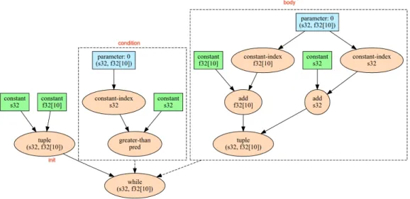
Tensorflow [3] is an open source ML framework for the Python program-ming language. Tensorflow aims to provide anything a developer may need to implement any deep learning model, and do so with high and portable performance. Creating a basic ML model such as Lenet [4] with Tensorflow only requires on the order of 10 lines of code. The most important part of Tensorflow for this work is the Accelerated Linear Algebra (XLA) compiler that is built into Tensorflow. By default, Tensorflow computation happens in the context of Tensorflow’s extensive dynamic runtime environment. The environment is dynamic in the sense that Python is an interpreted language. However, most Tensorflow operations, particularly computationally intensive operations such as matrix-matrix multiply and convolution, leverage libraries such as MKL to execute more efficiently than they would if implemented natively in Python. The XLA compiler is able to generate executable bi-naries for a particular ML model with only essential functions, avoiding the heavyweight runtime environment. The compiler can cross-compile for other architectures such as ARM, and the results are lightweight enough to be used on mobile devices and even wearables. XLA can outperform the li-braries in the default Tensorflow environment since the executable can be specialized to a particular ML model and optimizations can be performed across the boundaries between operations. While the libraries in the run time are highly optimized, they must be also general enough for any poten-tial invocation, a constraint not shared with XLA executables. In order to optimize a particular ML model, XLA uses an intermediate representation called High Level Optimizer (HLO), which is conceptually similar to LLVM’s IR discussed in section 2.4. HLO is a higher level representation than LLVM IR; it can represent operations at granularities from scalar addition up to multidimensional convolution operations, whereas LLVM IR can only repre-sent scalar and vector operations. Figure 2.1 gives an example of how HLO represents computation, the addition of a constant 10-element floating point vector to the input vector of the same type in a loop that is repeated a constant number of times. An optimization pass in HLO could potentially identify this repeated addition and apply a transformation similar to strength reduction in a traditional compiler like LLVM: the elements of the constant vector could be multiplied by the loop iteration count and the result of that

Figure 2.1: Visualization of HLO1

added to the input vector once, which would be a significant reduction in computation for large loop iteration counts. An optimization such as this would likely be impossible in a traditional compiler such as LLVM since the repeated addition operations would be obscured by a loop within the loop which loads in the value at some index of the input vectors from memory, adds the values together, and stores the result back to memory. HLO affords a level of abstraction where this sort of detail does not prevent substantial optimizations such as this example.

2.6 High Level Synthesis

HLS is the process of synthesizing hardware designs from high-level lan-guages such as C and C++. HLS tools automatically generate Verilog or other equivalent register-transfer logic (RTL) format, where traditionally an engineer would write the Verilog implementation directly. Designing digital hardware with RTL is more laborious than programming equivalent compu-tation in a high-level language such as C or C++. One work [5] reports a fivefold reduction in development effort. Another work [6] reports more mod-est reductions, or even a slight increase in one case, in development effort,

1_{Portions of this page are reproduced from work created and shared by Google (https:}

//www.tensorflow.org/xla/operation_semantics) and used according to terms de-scribed in the Creative Commons 3.0 Attribution License.

but with 11-31% reduction in resource usage. These results come from a tool expert who is focused on finely tuning the HLS quality of results (QoR). If performance and resource usage are not concerns, an experienced C/C++ programmer would certainly see closer to the fivefold reduced development effort compared to an experienced RTL designer. However, if high QoR is desired, expertise and longer development time are required. This is because HLS tools are unable to efficiently map naive or idiomatic code to a hard-ware implementation. The programmer must transform the source code in ways that lead the HLS tool to efficiently allocate resources and schedule operations. Common transformations include loop unrolling and pipelining directives (which are passed to the HLS tool in different ways for differ-ent tools, often a #pragma is used) which expose parallelism that the HLS tool knows how to exploit. Another more manual transformation is buffering data that will end up having to be read from off-chip memory in smaller local arrays which the HLS tool will synthesize as on-chip random access mem-ory (RAM) units. This can help if the data can be used more than once, thus eliminating the access latency of subsequent accesses. Also, ping-pong buffers can be used where one buffer is filled from main memory or written out to main memory while another buffer is being used for computation. The buffers swap tasks when both are finished, effectively hiding the latency ei-ther of interacting with memory or of the computation, whichever is shorter. In this work we will show that transformations such as these can be utilized without programmer intervention when taking a Tensorflow graph model of computation as input instead of C/C++ code.

2.6.1 LegUp HLS

LegUp [7] is an open-source HLS tool built as a backend target for LLVM. Besides the backend for Verilog RTL generation, LegUp also includes several compiler passes which perform LegUp-specific optimizations (such as loop pipelining discussed in section 3.2.1) and perform analysis needed during the RTL generation. LegUp has some powerful features such as the ability to extract parallelism from C code that uses the pthread library or OpenMP pragmatics. However, LegUp has some limitations that are common with HLS tools. For example, dynamic memory allocation, recursion and file

input and output are not able to be synthesized. LegUp can synthesize print statements for use in simulation only.

2.7 Related Work

Many previous works that leverage HLS for ML applications have focused on implementing the applications in HLS-friendly C/C++ code. Typically the models are first developed in a framework such as Caffe or Tensorflow by ML experts. These frameworks are designed for experts to design and train novel models, and are also capable of extracting the best performance from CPUs and GPUs without requiring expert programming by using existing libraries such as MKL and libraries included in the frameworks. However, these frameworks are not able to leverage the potential of custom hardware.

2.7.1 TPU

One exception is Google’s Tensor Processing Unit [8] (TPU). TPU is not customized or optimized for a particular model but is more specialized for ML computations than is a CPU or GPU. XLA is used to compile Tensorflow models for execution on TPUs. Only certain computations, namely matrix multiplication and other operations that can be efficiently reduced to matrix multiplication such as convolution, are compiled to run on the TPU. The remaining operations are executed on the host CPU. Typically these opera-tions are not as computationally intense as TPU-friendly operaopera-tions and are not the performance bottleneck.

2.7.2 LeFlow

In the LeFlow [9] work, a hardware backend for XLA is proposed. This back-end produces truly specialized hardware for a particular Tensorflow model. XLA’s CPU backend produces LLVM IR which can then be compiled for any architecture that has an existing LLVM backend. LeFlow uses LegUp as a Verilog RTL backend for XLA in place of the typical LLVM CPU backends. LeFlow takes a user’s Tensorflow code as input. The user’s input code

with the XLA CPU backend. This code is then executed on the host CPU and a configuration parameter set by LeFlow causes the LLVM IR file for the CPU execution to be saved in a particular directory. First, LeFlow down-grades the LLVM IR syntax from Tensorflow’s version (which uses LLVM 7) to LegUp’s version (LLVM 3.5, which was the most recent version the last time the open-source version of LegUp was updated) using string op-erations in Python. LeFlow then runs some standard LLVM optimizations on this IR, followed by flow-specific transformations implemented with string operations in Python. The first transformation renames the accelerated func-tion and removes some funcfunc-tion arguments (performance counters and run options) which are unused and transforms the remaining arguments to be global variables. LegUp allows for top-level functions to have arguments but this transformation is just a logistical matter; the authors preferred setting the values as global variables rather than passing them in as arguments. The second transformation rewrites an LLVM operation that is unsupported by LegUp into a form that is equivalent and supported. The third transforma-tion partitransforma-tions statically allocated arrays according to user input specified in a configuration file. The partitioning leads the HLS tool to synthesize the original array as separate block RAMs (BRAMs), which allows for parallel accesses. These transformations are also combined with LLVM and LegUp transformation passes and the resulting IR is finally synthesized with LegUp’s LLVM HLS backend into a Verilog RTL file.

CHAPTER 3

PROPOSED FLOW AND ARCHITECTURE

3.1 LegUp with LLVM 7.0

One of the contributions of this work is updating the LegUp HLS tool to work with LLVM version 7.0. As of this writing, the last public release of LegUp was in August 2015, three and a half years ago, and it was built on LLVM version 3.5. LLVM’s IR file format can change between versions, so the last released version of LegUp is only able to synthesize programs that were generated from tools built with LLVM 3.5 such as Clang 3.5, which is LLVM’s C/C++ frontend. Tensorflow uses a more recent version of LLVM so the IR it generates cannot be synthesized by LegUp as-is. The approach to this problem in LeFlow[9] was to transform the IR from the version 7.0 format to the 3.5 format using Python string operations. Unfortunately, al-though this approach requires less effort than upgrading LegUp to work with LLVM 7.0, it is highly sensitive to errors and the implementation provided (https://github.com/danielholanda/LeFlow) fails given reasonable inputs. A small example of the changes made to implement this transition is given in listing 5 in the appendix. The changes seen here are required because in LLVM 3.5, most iterators could be used as pointers to objects, whereas in LLVM 7.0, the iterators are not pointers and must be dereferenced to ob-tain an object (using the * operator), and the address of that object can be obtained with the&operator, the result of which may be used just as iterator-pointers were previously used in LLVM 3.5. Other changes were required as well, but this type of change was the most numerous.

Figure 3.1: Example scheduling of a pipelined loop

3.2 Optimizations

3.2.1 Loop Pipelining

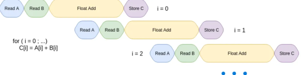
Loop pipelining is an HLS optimization analogous to software pipelining where instruction-level parallelism (ILP) is exploited across loop iteration boundaries. This optimization was implemented in LegUp previously and is leveraged in this work. Loop pipelining is similar to loop unrolling in that an unrolled loop is able to exploit most of the same ILP within the body of the unrolled loop, but the ILP between the end of one iteration and the beginning of the next is still not exploited without loop pipelining.

Figure 3.1 shows how a simple for loop could be pipelined by HLS. In a steady state, this solution achieves a twofold speedup over a serial, non-pipelined schedule. Note that the schedule could be even better if arrays A, B, and C were mapped to separate on-chip BRAMs which could be accessed simultaneously, though multiple floating point adders would be required to fully exploit the parallelism in that case. For simplicity, the example assumes the latency of the floating point adder is thrice the memory access latency. If the adder latency was longer, multiple adder instances could be used to over-come the structural hazard. If the adder latency was shorter, then accessing memory would be the bottleneck for the schedule unless, as mentioned, the array accesses could be scheduled simultaneously. The example typifies the algorithms that implement Tensorflow operations like matrix multiplication since they are also made up of loops with ILP that can be exploited across iteration boundaries.

3.2.2 Leveraging IPs

LegUp recursively translates function calls in the input program into instan-tiations of modules. Any function which is called but undefined in the input program will be also synthesized as a module instantiation under the assump-tion that an implementaassump-tion of the module will be given later. This allows hardware designers to use non-HLS Verilog modules as components in the larger HLS design.

As part of this work, the XLA CPU backend (which is used to generate the LLVM IR that is taken as input to the HLS flow) was leveraged to option-ally generate matrix multiply operations as a runtime library function call instead of generating the code to implement the operator’s computation. In LeFlow [9], the XLA CPU backend is modified to never emit these runtime library function calls since the runtime library is not present in hardware. In this work we instead create a flag to turn this functionality on or off. When enabled, the runtime library function call will be automatically synthesized into the instantiation of an intellectual property (IP) module. The module potentially implements the computation with better QoR than the HLS tool could have synthesized from the IR that the XLA CPU backend would have produced instead. Many of the arguments to the runtime library function are constants which give the dimensions of the input tensors and other param-eters such as whether an input should be considered as a transpose during computation. Given these constant parameters, the IP module can poten-tially be specialized (automatically or by hand) to a particular invocation, which would save the overhead involved with a more generic implementation.

3.3 Results

3.3.1 A Simple HLS IP for Matrix Multiplication

We compare and discuss various implementations of matrix multiplication of dimensions 7×101 and 101 ×23. Our baseline is an implementation

cre-ated by simply using LegUp to synthesize the LLVM IR emitted by XLA’s CPU backend without any use of IP modules. As a first step and proof of concept for the flow, a naive, non-specialized (conforming to XLA’s generic

Table 3.1: Comparison of various matrix multiplication implementations LEs MemB FMax Cycles Speedup

Non-IP 5,420 102,112 99.07 455,800 baseline

Basic HLS IP 3,015 102,112 180.6 489,243 1.7 Manually unrolled HLS IP 4,334 102,112 180.2 252,550 3.3 Handmade RTL IP 5,434 103,536 101.5 72,940 6.4

runtime library function) matrix multiply IP was created using LegUp HLS. The source code for the IP is shown in listing 1 in the appendix. The code gives a good example of how specialization can lead to better results. One can see how the input array index calculation depends on whether each input is transposed or not, adding overhead that would not be present in a spe-cialized IP. In table 3.1, we see that while the IP version takes more steps to implement the same computation, it more than makes up for the difference with a higher clock frequency, resulting in a1.7×speedup over our baseline.

We observe that for both the non-IP and HLS-IP implementations, LegUp is only able to create one of each floating point multiplication and floating point addition functional unit, despite being given resource constraints that allow for more than one of each. This signals that these implementations are not exploiting the parallelism inherent in the matrix multiplication algorithm as much as one would expect with custom hardware. In an attempt to alleviate this, the inner loop of the implementation shown in listing 1 was manually unrolled instead of relying on LLVM passes in the LegUp flow to unroll this loop. The result of this transformation can be found in listing 2. The resulting implementation still only uses one of each functional unit but the manual unrolling allows the HLS tool to find a better scheduling of the operations, resulting in a 1.93× relative speedup over the original HLS

IP. This is likely caused by the explicitly unrolled loop allowing LegUp HLS to overlap the scheduling of the unrolled loads, arithmetic operations, and stores. During testing, we observed that this implementation sacrifices some negligible amount of accuracy due to an adder tree used to efficiently sum the results of the unrolled iterations. Since floating point addition is not commutative, rearranging the order of floating point additions does not give exactly the same result, but it is within any reasonable tolerance for error.

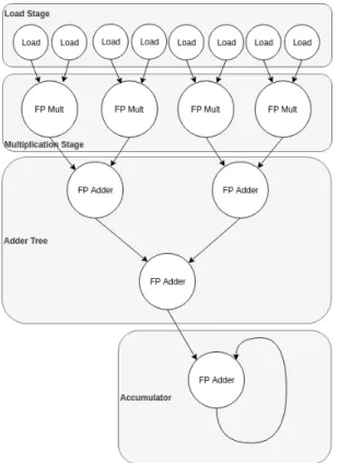
In addition to the HLS-generated IPs, our work can also leverage hand-made RTL IPs. As an example of this, a simple matrix multiply IP was

Figure 3.2: Matrix multiply RTL IP architecture

created by hand with SystemVerilog. The RTL IP uses four floating point multiplication functional units and four floating point addition units, three for an adder tree and one for an accumulator. The source code for the IP is given in listing 4 of the appendix and an architectural overview is given in figure 3.2. The computation is split into five stages: reading data in, multi-plication, two stages for the adder tree, and a final stage for accumulation. For simplicity, the result is simply stored while the stages are flushed and the output indices incremented appropriately - there is no explicit stage needed for storing the result. This implementation enjoys a 6.4× speedup over the

baseline and a 1.95×relative speedup over the manually unrolled HLS IP.

3.3.2 A Simple HLS IP for Max Pooling

In addition to matrix multiplication, using an HLS IP module for max pooling was also explored. Max pooling is an operation used in neural networks such as Lenet [4]. The output of max pooling at some index is the largest element within a window of the input at the strided index. For example taking a

Table 3.2: Comparison of max pooling results from LeFlow [9] LEs MemB FMax Cycles

LeFlow 8×8 981 2,176 221.43 229

LeFlow 32×32 979 35,968 219.25 5,533

Ours 8×8 3,431 2,560 179.82 883

Ours 32×32 3,434 40,960 179.82 13,663

4×4matrix as input, the result of 2×2-windowed and strided max pooling

would be a 2×2 matrix with elements equal to the largest elements of the

four 2×2submatrices of the input. The stride is often the same size as the

window as in this example, so there is typically no overlap between strided windows, but this is not a requirement in a generic implementation. As with the first IP explored in section 3.3.1, the max pooling IP was implemented using LegUp HLS. The source code for the implementation is given in listing 3. This code is also not specially optimized for HLS and is generic in the size of the dimensions, window, and stride. Unlike the matrix multiplication IP, this IP is not able to overcome the overhead incurred by this generality.

Table 3.2 shows a comparison of two benchmarks reported in LeFlow [9] to our IP-based implementation. The benchmarks are 2×2-windowed and

strided max pooling on8×8and32×32single precision floating point inputs,

for which we observe a slowdown factor of0.21×and0.33×, respectively. The

differences in maximum clock frequency can be explained by LeFlow likely using LegUp’s default behavior of not giving timing constraints for top-level inputs and outputs. This leads to unconstrained paths in the design, mean-ing the results of timmean-ing analysis are not well defined and the higher clock frequencies are not necessarily meaningful. On the other hand, by setting input and output delays with the accelerator as the top-level module, the maximum frequency is likely worse (though it is well defined) than in a real-world design which instantiates the accelerator as a component. In addition to matrix multiply and max pooling, other compute-intensive operations such as convolution and fast Fourier transform could also be supported.

CHAPTER 4

CONCLUSION

4.1 Future Work

With continued effort, several further improvements to this work are possi-ble. Performance improvements will likely be realized if the XLA LLVM IR generation is modified to generate more HLS-friendly IR. The intuition here is that an experienced HLS user seeking better QoR knows how to trans-form their code in ways that an automatic compiler transtrans-formation cannot. One could build this sort of intuition into the XLA LLVM IR generation. Additionally, the results in section 3.3.1 are a simple proof of concept with potential for improvement. It is our view that most Tensorflow applications will see a greater performance improvement with more highly tuned IPs sup-porting the most computation-intensive operations than with an improved, HLS-friendly, XLA LLVM IR backend. However, both are promising frontiers for future work.

4.2 Summary

HLS allows users to leverage custom hardware with higher productivity than traditional hardware at some expense of performance. FPGAs enable users to cheaply take advantage of the multitude of custom accelerator designs avail-able through HLS. Our work demonstrates how users can accelerate machine learning applications using Tensorflow instead of the traditional C/C++ ap-proach to HLS, providing even greater improvements in productivity. We have also demonstrated how this approach can effortlessly provide non-expert users with QoR traditionally only achieved by hardworking HLS experts.

REFERENCES

[1] S. Cass, “The 2017 top programming languages,” Piscataway, NJ, USA, 2017. [Online]. Available: https://spectrum.ieee.org/computing/ software/the-2017-top-programming-languages

[2] C. Lattner and V. Adve, “LLVM: A compilation framework for lifelong program analysis & transformation,” in Proceedings of the International Symposium on Code Generation and Optimization: Feedback-directed and Runtime Optimization, ser. CGO ’04. Washington, DC, USA: IEEE Computer Society, 2004. [Online]. Available: http: //dl.acm.org/citation.cfm?id=977395.977673

[3] M. Abadi, A. Agarwal, P. Barham, E. Brevdo, Z. Chen, C. Citro, G. S. Corrado, A. Davis, J. Dean, M. Devin, S. Ghemawat, I. Goodfellow, A. Harp, G. Irving, M. Isard, Y. Jia, R. Jozefowicz, L. Kaiser, M. Kudlur, J. Levenberg, D. Mané, R. Monga, S. Moore, D. Murray, C. Olah, M. Schuster, J. Shlens, B. Steiner, I. Sutskever, K. Talwar, P. Tucker, V. Vanhoucke, V. Vasudevan, F. Viégas, O. Vinyals, P. Warden, M. Wattenberg, M. Wicke, Y. Yu, and X. Zheng, “TensorFlow: Large-scale machine learning on heterogeneous systems,” 2015, software available from tensorflow.org. [Online]. Available: https://www.tensorflow.org/

[4] Y. Lecun, L. Bottou, Y. Bengio, and P. Haffner, “Gradient-based learning applied to document recognition,” in Proceedings of the IEEE, 1998, pp. 2278–2324.

[5] Y. Liang, K. Rupnow, Y. Li, D. Min, M. N. Do, and D. Chen, “High-level synthesis: Productivity, performance, and software constraints,” JECE, Jan. 2012. [Online]. Available: http://dx.doi.org/10.1155/2012/649057 [6] J. Cong, B. Liu, S. Neuendorffer, J. Noguera, K. Vissers, and Z. Zhang,

“High-level synthesis for FPGAs: From prototyping to deployment,” IEEE TCAD, p. 491, 2011.

[7] A. Canis, J. Choi, B. Fort, R. Lian, Q. Huang, N. Calagar, M. Gort, J. Jun Qin, M. Aldham, T. Czajkowski, S. Brown, and J. Anderson, “From software to accelerators with legup high-level synthesis,” in 2013 International Conference on Compilers, Architecture and Synthesis for Embedded Systems, CASES 2013, 09 2013, pp. 1–9.

[8] N. P. Jouppi, C. Young, N. Patil, D. A. Patterson, G. Agrawal, R. Bajwa, S. Bates, S. Bhatia, N. Boden, A. Borchers, R. Boyle, P. Cantin, C. Chao, C. Clark, J. Coriell, M. Daley, M. Dau, J. Dean, B. Gelb, T. V. Ghaemmaghami, R. Gottipati, W. Gulland, R. Hagmann, R. C. Ho, D. Hogberg, J. Hu, R. Hundt, D. Hurt, J. Ibarz, A. Jaffey, A. Jaworski, A. Kaplan, H. Khaitan, A. Koch, N. Kumar, S. Lacy, J. Laudon, J. Law, D. Le, C. Leary, Z. Liu, K. Lucke, A. Lundin, G. MacKean, A. Maggiore, M. Mahony, K. Miller, R. Nagarajan, R. Narayanaswami, R. Ni, K. Nix, T. Norrie, M. Omernick, N. Penukonda, A. Phelps, J. Ross, A. Salek, E. Samadiani, C. Severn, G. Sizikov, M. Snelham, J. Souter, D. Steinberg, A. Swing, M. Tan, G. Thorson, B. Tian, H. Toma, E. Tuttle, V. Vasudevan, R. Walter, W. Wang, E. Wilcox, and D. H. Yoon, “In-datacenter performance analysis of a tensor processing unit,” CoRR, 2017. [Online]. Available: http://arxiv.org/abs/1704.04760 [9] D. H. Noronha, B. Salehpour, and S. J. E. Wilton, “LeFlow: Enabling flexible FPGA high-level synthesis of tensorflow deep neural networks,” CoRR, 2018. [Online]. Available: http://arxiv.org/abs/1807.05317

APPENDIX

SELECTED SOURCE CODE LISTINGS

This appendix contains source code relevant to the project. Listing 1: Eigen matrix multiply IP source code

#include <stdint . h>

void EigenMatMulF32(void ∗_, float ∗out , float ∗lhs , float ∗rhs , int64_t m, int64_t n , int64_t k , int32_t transpose_lhs , int32_t transpose_rhs ) { int64_t i , j , kk , lhs_idx , rhs_idx ;

float tmp; for ( i = 0; i < m; i++) { for ( j = 0; j < n ; j++) { tmp = 0 . 0 ; for (kk = 0; kk < k ; kk++) { lhs_idx = transpose_lhs ? (( i ∗k) + kk) : (( kk∗m) + i ) ; rhs_idx = transpose_rhs ? (( kk∗n) + j ) : (( j ∗k) + kk ) ; tmp += lhs [ lhs_idx ] ∗ rhs [ rhs_idx ] ; } out [ ( j ∗m) + i ] = tmp; } } }

Listing 2: Manually unrolled matrix multiply source code

#include <stdint . h>

void __xla_cpu_runtime_EigenMatMulF32(void ∗_, float ∗out , float ∗lhs , float ∗rhs , int64_t m, int64_t n , int64_t k , int32_t transpose_lhs , int32_t transpose_rhs ) {

int64_t i , j , kk , lhs_idx , rhs_idx ;

float tmp, tmp1 , tmp2 , tmp3 , tmp4 , tmp5 , tmp6 , tmp7 ; for ( i = 0; i < m; i++) { for ( j = 0; j < n ; j++) { tmp = 0 . 0 ; kk = 0; for ( ; kk < (k−4);) { lhs_idx = transpose_lhs ? (( i ∗k) + kk) : (( kk∗m) + i ) ; rhs_idx = transpose_rhs ? (( kk∗n) + j ) : (( j ∗k) + kk ) ; tmp1 = lhs [ lhs_idx ] ∗ rhs [ rhs_idx ] ; kk++; lhs_idx = transpose_lhs ? (( i ∗k) + kk) : (( kk∗m) + i ) ;

rhs_idx = transpose_rhs ? (( kk∗n) + j ) : (( j ∗k) + kk ) ; tmp2 = lhs [ lhs_idx ] ∗ rhs [ rhs_idx ] ; kk++; lhs_idx = transpose_lhs ? (( i ∗k) + kk) : (( kk∗m) + i ) ; rhs_idx = transpose_rhs ? (( kk∗n) + j ) : (( j ∗k) + kk ) ; tmp3 = lhs [ lhs_idx ] ∗ rhs [ rhs_idx ] ; kk++; lhs_idx = transpose_lhs ? (( i ∗k) + kk) : (( kk∗m) + i ) ; rhs_idx = transpose_rhs ? (( kk∗n) + j ) : (( j ∗k) + kk ) ; tmp4 = lhs [ lhs_idx ] ∗ rhs [ rhs_idx ] ; kk++; tmp5 = tmp1 + tmp2 ; tmp6 = tmp3 + tmp4 ; tmp7 = tmp5 + tmp6 ; tmp = tmp + tmp7 ; } for ( ; kk < k ; kk++) { lhs_idx = transpose_lhs ? (( i ∗k) + kk) : (( kk∗m) + i ) ; rhs_idx = transpose_rhs ? (( kk∗n) + j ) : (( j ∗k) + kk ) ; tmp += lhs [ lhs_idx ] ∗ rhs [ rhs_idx ] ; } out [ ( j ∗m) + i ] = tmp; } } }

Listing 3: Max pooling IP source code

#include <stdint . h>

#include <math . h>

void max_pool_ip(float ∗out , float ∗in ,

int64_t ip , int64_t iz , int64_t iy , int64_t ix , //input dimensions

int64_t op , int64_t oz , int64_t oy , int64_t ox , //output dimensions

int64_t wp, int64_t wz, int64_t wy, int64_t wx, //window dimensions

int64_t sp , int64_t sz , int64_t sy , int64_t sx , //window s t r i d e

int64_t pp , int64_t pz , int64_t py , int64_t px //window padding low

) {

int64_t i i , i j , ik , i l ; //input indices

int64_t oi , oj , ok , ol ; //output indices

int64_t bi , bj , bk , bl ; //window begin

int64_t ei , ej , ek , e l ; //window end

int64_t o_idx , i_idx ; // l i n e a r i z e d output and input indices

float tmp1 , tmp2 ;

for ( ol = 0; ol < ox ; ol++) { //dim(3) i s x i s most minor dimension

for (ok = 0; ok < oy ; ok++) {

for ( oj = 0; oj < oz ; oj++) {

for ( oi = 0; oi < op ; oi++) { //dim(0) i s p i s most major dimension

tmp1 =−INFINITY;

bl = (( ol ∗sx ) − px) > 0 ? (( ol ∗sx ) − px) : 0;

bk = (( ok∗sy ) − py) > 0 ? (( ok∗sy ) − py) : 0;

e l = (( ol ∗sx ) + wx− px) < ix ? (( ol ∗sx ) + wx− px) : ix ;

ek = (( ok∗sy ) + wy− py) < iy ? (( ok∗sy ) + wy− py) : iy ;

ej = (( oj ∗ sz ) + wz− pz ) < i z ? (( oj ∗ sz ) + wz− pz ) : i z ;

e i = (( oi ∗sp ) + wp− pp) < ip ? (( oi ∗sp ) + wp− pp) : ip ;

o_idx = (oy∗oz∗op∗ ol ) + ( oz∗op∗ok) + (op∗ oj ) + oi ;

for ( i l = bl ; i l < e l ; i l ++) { for ( ik = bk ; ik < ek ; ik++) { for ( i j = bj ; i j < e j ; i j++) { for ( i i = bi ; i i < e i ; i i ++) { i_idx = ( iy ∗ i z ∗ ip ∗ i l ) + ( i z ∗ ip ∗ ik ) + ( ip ∗ i j ) + i i ; tmp2 = in [ i_idx ] ; tmp1 = tmp1 > tmp2 ? tmp1 : tmp2 ; } } } } out [ o_idx ] = tmp1 ; } } } } }

Listing 4: Handwritten RTL IP for matrix multiplication

‘define MEMORY_CONTROLLER_ADDR_SIZE 64 ‘define MEMORY_CONTROLLER_DATA_SIZE 64 ‘define MULT_CYCLES 64 ’d11 ‘define ADD_CYCLES 64 ’d14 module MatMulRTLIP ( clk , reset , start , f i n i s h , memory_controller_waitrequest , memory_controller_enable_a , memory_controller_address_a , memory_controller_write_enable_a , memory_controller_in_a , memory_controller_size_a , memory_controller_out_a , memory_controller_enable_b , memory_controller_address_b , memory_controller_write_enable_b , memory_controller_in_b , memory_controller_size_b , memory_controller_out_b , arg_out , arg_lhs , arg_rhs ) ;

input clk ; input r e s e t ; input s t a r t ; output l o g i c f i n i s h ; input memory_controller_waitrequest ; output l o g i c memory_controller_enable_a ;

output l o g i c [‘MEMORY_CONTROLLER_ADDR_SIZE−1:0] memory_controller_address_a ;

output l o g i c memory_controller_write_enable_a ;

output l o g i c [‘MEMORY_CONTROLLER_DATA_SIZE−1:0] memory_controller_in_a ;

output l o g i c [ 1 : 0 ] memory_controller_size_a ;

input [‘MEMORY_CONTROLLER_DATA_SIZE−1:0] memory_controller_out_a ;

output l o g i c memory_controller_enable_b ;

output l o g i c [‘MEMORY_CONTROLLER_ADDR_SIZE−1:0] memory_controller_address_b ;

output l o g i c memory_controller_write_enable_b ;

output l o g i c [‘MEMORY_CONTROLLER_DATA_SIZE−1:0] memory_controller_in_b ;

output l o g i c [ 1 : 0 ] memory_controller_size_b ;

input [‘MEMORY_CONTROLLER_DATA_SIZE−1:0] memory_controller_out_b ;

input [‘MEMORY_CONTROLLER_ADDR_SIZE−1:0] arg_out ;

input [‘MEMORY_CONTROLLER_ADDR_SIZE−1:0] arg_lhs ;

input [‘MEMORY_CONTROLLER_ADDR_SIZE−1:0] arg_rhs ;

parameter [ 6 3 : 0 ] arg_m;

parameter [ 6 3 : 0 ] arg_n ;

parameter [ 6 3 : 0 ] arg_k ;

parameter [ 3 1 : 0 ] arg_transpose_lhs ;

parameter [ 3 1 : 0 ] arg_transpose_rhs ; enum int unsigned {

idle , in it , accumulate , write , reset_pipeline } state , next_state ; // i t e r a t i o n variables reg [ 6 3 : 0 ] i ; reg [ 6 3 : 0 ] j ; reg [ 6 3 : 0 ] k ; //address variables l o g i c [‘MEMORY_CONTROLLER_ADDR_SIZE−1:0] reset_addr_left ; l o g i c [‘MEMORY_CONTROLLER_ADDR_SIZE−1:0] reset_addr_right ; l o g i c [‘MEMORY_CONTROLLER_ADDR_SIZE−1:0] next_addr_left ; l o g i c [‘MEMORY_CONTROLLER_ADDR_SIZE−1:0] next_addr_right ;

wire [‘MEMORY_CONTROLLER_ADDR_SIZE−1:0] out_addr ;

reg [‘MEMORY_CONTROLLER_ADDR_SIZE−1:0] addr_left ;

reg [‘MEMORY_CONTROLLER_ADDR_SIZE−1:0] addr_right ;

// f l o a t i n g point r e g i s t e r s

reg [ 3 1 : 0 ] load_stage_a [ 3 : 0 ] ;

reg [ 3 1 : 0 ] mult_b [ 3 : 0 ] ; wire [ 3 1 : 0 ] mult_out [ 3 : 0 ] ; reg [ 3 1 : 0 ] adder_tree_0_in [ 3 : 0 ] ; wire [ 3 1 : 0 ] adder_tree_0_out [ 1 : 0 ] ; reg [ 3 1 : 0 ] adder_tree_1_in [ 1 : 0 ] ; wire [ 3 1 : 0 ] adder_tree_1_out ; wire [ 3 1 : 0 ] accumulator_out ; reg [ 3 1 : 0 ] accumulator_in ; reg [ 3 1 : 0 ] accumulator ; // control signal s reg [ 3 : 0 ] mult_state ; reg [ 3 : 0 ] add_state ; reg [ 2 : 0 ] load_state ; reg [ 3 : 0 ] load_valid ; reg [ 3 : 0 ] mult_valid ; reg [ 1 : 0 ] add_0_valid ; reg add_1_valid ; reg acc_valid ;

wire mult_done , add_done , load_done ;

wire load_move_forward ;

wire pipeline_move_forward ; l o g i c k_reset ;

l o g i c inc_ij ;

//some helper signal s

assign load_valid [ 0 ] = k < arg_k ;

assign load_valid [ 1 ] = k < (arg_k− 64 ’h1 ) ;

assign load_valid [ 2 ] = k < (arg_k− 64 ’h2 ) ;

assign load_valid [ 3 ] = k < (arg_k− 64 ’h3 ) ;

assign mult_done = mult_state >= ‘MULT_CYCLES;

assign add_done = add_state >= ‘ADD_CYCLES;

assign load_done = load_state >= 64 ’d6 ;

assign load_move_forward = ( ! memory_controller_waitrequest ) & ! load_done ;

assign pipeline_move_forward = add_done && mult_done && load_done ;

assign out_addr = arg_out + {( j ∗ arg_m) + i , 2 ’b00 };

assign memory_controller_in_a = accumulator ;

assign memory_controller_address_b = addr_right ;

assign memory_controller_write_enable_b = 1 ’b0 ; assign memory_controller_in_b = 0; assign memory_controller_size_a = 2 ’h2 ; assign memory_controller_size_b = 2 ’h2 ; //transpose indexing l o g i c always_comb begin i f ( arg_transpose_lhs ) begin

reset_addr_left = arg_lhs + { i ∗ arg_k , 2 ’b00 }; next_addr_left = addr_left + 64 ’h4 ;

end else begin

reset_addr_left = arg_lhs + { i , 2 ’b00 }; next_addr_left = addr_left + {arg_m, 2 ’b00 };

end

i f ( arg_transpose_rhs ) begin

next_addr_right = addr_right + {arg_n , 2 ’b00 };

end else begin

reset_addr_right = arg_rhs + { j ∗ arg_k , 2 ’b00 }; next_addr_right = addr_right + 64 ’h4 ;

end end

//next_state and control l o g i c

always_comb begin next_state = state ; f i n i s h = 1 ’b0 ; k_reset = 1 ’b0 ; inc_ij = 1 ’b0 ; memory_controller_address_a = addr_left ; memory_controller_enable_a = 1 ’b0 ; memory_controller_enable_b = 1 ’b0 ; memory_controller_write_enable_a = 1 ’b0 ; case ( state ) i d l e : begin i f ( s t a r t ) begin next_state = i n i t ; end end i n i t : begin k_reset = 1 ’b1 ; next_state = accumulate ; end accumulate : begin

i f ( ( ! acc_valid ) && ( ! add_1_valid) && ( ! ( | add_0_valid )) && ( ! ( | mult_valid )) && ( ! ( | load_valid ) ) ) begin

next_state = write ;

end

memory_controller_enable_a = load_valid [ load_state [ 1 : 0 ] ] & ( ! load_state [ 2 ] ) ; memory_controller_enable_b = load_valid [ load_state [ 1 : 0 ] ] & ( ! load_state [ 2 ] ) ;

end write : begin memory_controller_enable_a = 1 ’b1 ; memory_controller_write_enable_a = 1 ’b1 ; memory_controller_address_a = out_addr ; i f ( ! memory_controller_waitrequest ) begin inc_ij = 1 ’b1 ; next_state = reset_pipeline ; end end reset_pipeline : begin i f ( i == arg_m) begin next_state = i d l e ; f i n i s h = 1 ’b1 ;

end else begin

next_state = accumulate ; k_reset = 1 ’b1 ;

end end

end

// i t e r a t o r l o g i c

always @(posedge clk ) begin

i f ( s t a r t | ( state == i n i t )) begin

i <= 64 ’h0 ; j <= 64 ’h0 ;

end else i f ( inc_ij && ( j == (arg_n− 64 ’h1 ) ) ) begin

i <= i + 64 ’h1 ; j <= 64 ’h0 ;

end else i f ( inc_ij ) begin

j <= j + 64 ’h1 ;

end end

//load stage

always @(posedge clk ) begin i f ( k_reset ) begin

load_state <= 3 ’h0 ;

addr_left <= reset_addr_left ; addr_right <= reset_addr_right ;

end else i f (load_move_forward) begin i f ( ! load_state [ 2 ] ) begin

addr_left <= next_addr_left ; addr_right <= next_addr_right ;

end

for ( int i = 0; i < 4; i ++) begin i f ( load_state == ( i +2)) begin load_stage_a [ i ] <= memory_controller_out_a ; load_stage_b [ i ] <= memory_controller_out_b ; end end load_state <= load_state + 3 ’h1 ;

end else i f ( pipeline_move_forward ) begin

load_state <= 3 ’h0 ;

end end

// arithmetic pipeline

always @(posedge clk ) begin i f ( k_reset ) begin k <= 64 ’h0 ; mult_state <= 4 ’h0 ; add_state <= 4 ’h0 ; acc_valid <= 1 ’b0 ; mult_valid <= 4 ’h0 ; add_1_valid <= 1 ’b0 ; add_0_valid <= 2 ’h0 ; mult_valid <= 4 ’h0 ; accumulator <= 32 ’h0 ;

for ( int i = 0; i < 4; i++) begin

adder_tree_0_in [ i ] <= 32 ’h0 ; mult_a [ i ] <= 32 ’h0 ;

end

adder_tree_1_in [ 0 ] <= 32 ’h0 ; adder_tree_1_in [ 1 ] <= 32 ’h0 ; accumulator_in <= 32 ’h0 ;

end else i f ( pipeline_move_forward ) begin

k <= k + 64 ’h4 ;

mult_a <= load_stage_a ; mult_b <= load_stage_b ;

adder_tree_0_in [ 0 ] <= mult_valid [ 0 ] ? mult_out [ 0 ] : 32 ’h0 ; adder_tree_0_in [ 1 ] <= mult_valid [ 1 ] ? mult_out [ 1 ] : 32 ’h0 ; adder_tree_0_in [ 2 ] <= mult_valid [ 2 ] ? mult_out [ 2 ] : 32 ’h0 ; adder_tree_0_in [ 3 ] <= mult_valid [ 3 ] ? mult_out [ 3 ] : 32 ’h0 ; adder_tree_1_in <= adder_tree_0_out ; accumulator_in <= adder_tree_1_out ; accumulator <= accumulator_out ; mult_state <= 4 ’h0 ; add_state <= 4 ’h0 ; add_0_valid [ 0 ] <= | mult_valid [ 1 : 0 ] ; add_0_valid [ 1 ] <= | mult_valid [ 3 : 2 ] ; add_1_valid <= | add_0_valid ; acc_valid <= add_1_valid ; mult_valid <= load_valid ;

end else begin

i f ( mult_state < ‘MULT_CYCLES) begin

mult_state <= mult_state + 4 ’h1 ;

end

i f ( add_state < ‘ADD_CYCLES) begin

add_state <= add_state + 4 ’h1 ; end end end altfp_multiplier_11 multipliers0 ( . r e s u l t (mult_out [ 0 ] ) , . dataa (mult_a [ 0 ] ) , . datab (mult_b [ 0 ] ) , . clock ( clk ) , . clk_en ( ! mult_done) ) ; altfp_multiplier_11 multipliers1 ( . r e s u l t (mult_out [ 1 ] ) , . dataa (mult_a [ 1 ] ) , . datab (mult_b [ 1 ] ) , . clock ( clk ) , . clk_en ( ! mult_done) ) ; altfp_multiplier_11 multipliers2 ( . r e s u l t (mult_out [ 2 ] ) , . dataa (mult_a [ 2 ] ) , . datab (mult_b [ 2 ] ) , . clock ( clk ) ,

) ; altfp_multiplier_11 multipliers3 ( . r e s u l t (mult_out [ 3 ] ) , . dataa (mult_a [ 3 ] ) , . datab (mult_b [ 3 ] ) , . clock ( clk ) , . clk_en ( ! mult_done) ) ; altfp_adder_14 adder_tree_00 ( . r e s u l t ( adder_tree_0_out [ 0 ] ) , . dataa ( adder_tree_0_in [ 1 ] ) , . datab ( adder_tree_0_in [ 3 ] ) , . clock ( clk ) , . clk_en ( ! add_done) ) ; altfp_adder_14 adder_tree_01 ( . r e s u l t ( adder_tree_0_out [ 1 ] ) , . dataa ( adder_tree_0_in [ 0 ] ) , . datab ( adder_tree_0_in [ 2 ] ) , . clock ( clk ) , . clk_en ( ! add_done) ) ; altfp_adder_14 adder_tree_1 ( . r e s u l t ( adder_tree_1_out ) , . dataa ( adder_tree_1_in [ 0 ] ) , . datab ( adder_tree_1_in [ 1 ] ) , . clock ( clk ) , . clk_en ( ! add_done) ) ; altfp_adder_14 accumulator_adder ( . r e s u l t ( accumulator_out ) , . dataa ( accumulator_in ) , . datab ( accumulator ) , . clock ( clk ) , . clk_en ( ! add_done) ) ; always_ff @(posedge clk ) begin i f ( r e s e t ) begin state <= i d l e ;

end else begin

state <= next_state ;

end end endmodule

Listing 5: Example git diff for a LegUp file updated from LLVM 3.5 to 7.0 −−−a/lib/Transforms/LegUp/CustomVerilog.cpp

+++ b/lib/Transforms/LegUp/CustomVerilog.cpp

@@−74,7 +74,7 @@voidremoveBasicBlocksFromFunction(Function &F) { }

}

− BasicBlock ∗toRemove = &(∗(b++)); + BasicBlock ∗toRemove = b++;

toRemove−>removeFromParent();

}

@@−109,7 +109,7 @@voidremoveUncalledFunctionsFromVector(Function ∗function , std : : vector<FunctionW

for (Function : : iterator b = function−>begin() , be = function−>end(); b != be; ++b) {

for(BasicBlock : : iterator instr = b−>begin() , ie = b−>end(); instr != ie ; ++instr ) {

− if (isaDummyCall(&(∗instr )))continue; + if (isaDummyCall( instr ))continue;

if (CallInst ∗CI = dyn_cast<CallInst>(instr )) { Function ∗called = getCalledFunction(CI);

@@−158,7 +158,7 @@voidremoveFunctionsFromVectorIfNotCalled(std : : vector<Function ∗> &functions) {

for(Function : : iterator b = (∗ it)−>begin() , be = (∗ it)−>end(); b != be; ++b) {

for (BasicBlock : : iterator instr = b−>begin() , ie = b−>end(); instr != ie ; ++instr ) {

− if (isaDummyCall(&(∗instr ))) continue; + if (isaDummyCall( instr ))continue;

if (CallInst ∗CI = dyn_cast<CallInst>(instr )) { Function ∗called = getCalledFunction(CI); @@−265,7 +265,7 @@voidwarnIfCustomVerilogNotCalled(Module &M) {

for (Module: : iterator I = M. begin() , E = M.end(); I != E; ++I ) {

if (LEGUP_CONFIG−>isCustomVerilog(∗I )) { − cvFunctions.push_back(&(∗I )); + cvFunctions.push_back( I );

} }

@@−277,7 +277,7 @@voidwarnIfCustomVerilogNotCalled(Module &M) {

for(Function : : iterator b = it−>begin() , be = it−>end(); b != be; ++b) {

for (BasicBlock : : iterator instr = b−>begin() , ie = b−>end(); instr != ie ; ++instr ) {

− if (isaDummyCall(&(∗instr ))) continue; + if (isaDummyCall( instr ))continue;

if (CallInst ∗CI = dyn_cast<CallInst>(instr )) { Function ∗called = getCalledFunction(CI);

@@−353,7 +353,7 @@voidCustomVerilog : : getNonCustomVerilogFunctions(Module &M,

for (Module: : iterator I = M. begin() , E = M.end(); I != E; ++I ) {

if (!LEGUP_CONFIG−>isCustomVerilog(∗I )) { − HwFcts.push_back(&(∗I )); + HwFcts.push_back( I ); } } }

@@−363,7 +363,7 @@voidCustomVerilog : : getCustomVerilogFunctions(Module &M,

for (Module: : iterator I = M. begin() , E = M.end(); I != E; ++I ) {

if (LEGUP_CONFIG−>isCustomVerilog(∗I )) { − HwFcts.push_back(&(∗I )); + HwFcts.push_back( I ); } } }