Oil price forecasting using gene expression programming and artificial neural networks

(1)

Mohamed M. Mostafa

a,

_⁎

_{, Ahmed A. El-Masry}

b,c a_{College of Business, Gulf University for Science and Technology, West Mishref, Kuwait} b_{Plymouth Business School, UK Mansoura University, Egypt}

c_{Umm Al-Qura University, Saudi Arabia}

a b s t r a c t

a r t i c l e i n f o

Article history:

Accepted 16 December 2015 Available online xxxx

This study aims to forecast oil prices using evolutionary techniques such as gene expression programming (GEP) and artiﬁcial neural network (NN) models to predict oil prices over the period from January 2, 1986 to June 12, 2012. Autoregressive integrated moving average (ARIMA) models are employed to benchmark evolutionary models. The results reveal that the GEP technique outperforms traditional statistical techniques in predicting oil prices. Further, the GEP model outperforms the NN and the ARIMA models in terms of the mean squared error, the root mean squared error and the mean absolute error. Finally, the GEP model also has the highest explanatory power as measured by the R-squared statistic. The results of this study have important implications for both theory and practice.

Keywords:

Oil price prediction Gene expression programming Neural networks

ARIMA

1. Introduction

Crude oil holds an important and growing role in the world economy as about two thirds of the world's energy demand is met from crude oil (Alvarez-Ramirez et al., 2003). It is documented that crude oil is also the world's largest and most actively traded commodity, accounting for over 10% of total world trade (Verleger, 1993). Crude oil price, like most commodities, is basically determined by supply and demand (Hagen, 1994; Stevens, 1995), it is also affected by many irregular events such as weather, stock levels, GDP growth, political aspects and even people's psychological expectations. Since crude oil takes a consid-erable time to be shipped from one country to another, oil prices vary in different parts of the world. These factors lead to a stronglyfluctuating crude oil market, which has the characteristics of complex nonlinearity, dynamic variation and high irregularity (Watkins and Plourde, 1994). In addition, as sharp oil price movements can disturb aggregate economic activity, crude oil pricefluctuations may have a significant impact on a nation's economy. Therefore, volatile oil prices are of considerable inter-est to many institutions and business practitioners, as well as academic researchers. As such, crude oil price forecasting is a very important topic, albeit an extremely hard one, due to its intrinsic difficulties and high volatility (Wang et al., 2005). Oil price prediction has always proved to be an intractable task due to the intrinsic complexity of oil market mechanisms. In addition, the recent oil shocks and their far-reaching consequences have renewed the debate on understanding the behavior underlying oil prices.

Past studies have demonstrated a relationship between oil price and the GDP growth rate.Hamilton (1983)asserted that this relationship is asymmetric. He argued that the significant impacts on the economy can be observed only through a high increase in the price of oil. Hamilton's results have been confirmed by several subsequent studies. For example,Gisser and Goodwin (1986)indicated for the analyzed period from 1961 to 1982 that the oil price had its potential to predict GNP growth. Moreover, two interesting results concerning the relationship between oil price changes and macroeconomic variables are shown. First, the authors showed that monetary andfiscal policy measures alone cannot explain the effects of oil price shocks on macroeconomy after oil market disruptions. Thus, oil shocks also have an impact on economic output by other means than inflationary cost-push effects. Second, oil price effects on the U.S. economy did not change after 1973 when the OPEC period began. Hooker (1996) confirmed Hamilton's results and demonstrated that the oil price level and its changes do exert influence on GDP growth for the period 1948–1972. The author found that an increase of 10% in oil prices leads to a GDP growth of roughly 0.6 % lower in the third and fourth quarters after the shock. By investigating the relationship between GNP growth and oil price changes and volatility,Hamilton (2003)concluded that there is no doubt about the negative impact of oil price hikes and oil price volatility on economic growth during the last decades.

Narayan et al. (2014) investigated the role of oil price in the prediction of economic growth. The authors analyzed the data of 17 developing countries and 28 developed countries. Theﬁndings showed a higher level of predictability in case of developed countries.

Driesprong et al. (2008)investigated whether changes in oil price are good predictors of returns in stock market. The authors found

⁎ Corresponding author.

E-mail address:[email protected](M.M. Mostafa).

(2)

significant predictability in emerging markets as well as developed markets. The study also found that the introduction of lags of trading days plays a pivotal role in the relationship between oil price changes and stock returns.Pradhan et al. (2015)examined the relationship between economic growth, oil prices, depth in the stock market, real effective exchange rate, inflation rate, and real rate of interest using a panel vector autoregressive model to test Granger causality for the G-20 countries over the period 1961–2012. The results showed a robust long-run economic relationship between economic growth, oil prices, stock market depth, real effective exchange rate, inflation rate, and real rate of interest. While the study found that the empirical evidence of short-run causality is mixed, there was clear evidence that real economic growth responds to various measures of stock market depth, allowing for real oil price movements and changes in the real effective exchange rate, inflation rate, and real rate of interest.

In addition, previous studies have also investigated the link between oil price andfirm stock return.Jones and Kaul (1996)belong to thefirst authors to analyze the reaction of international stock markets to oil shocks by current and future changes in real cashflows and/or changes in expected returns. Their study considered stock markets in the US, Canada, UK and Japan, taking different institutional and regulatory environments into account. Except for the UK, oil prices were able to predict stock returns and output through 1991 in the other three coun-tries. Sadorsky's analysis showed that an oil price shock has a negative and statistically significant initial impact on stock returns.Papapetrou (2001)found that real stock returns are affected negatively. This impact lasts for approximately four months.Ciner (2001)extended existing studies on the relationship between oil prices and the stock market by testing for nonlinear linkages considering recent works on this subject (Hamilton, 1996). Prior studies as the one byHung et al. (1996)provide evidence for a significant causality between oil futures and stocks of individual companies, but showed no impact on a broad-based index like the S&P 500.Narayan and Sharma (2014)investigated whether the oil price contributes to stock return volatility in 560firms listed on the NYSE using daily data from January 2000 to 31 December 2008. The study found that oil price is a significant determinant and predictor offirms' returns variance. The study results indicated that investors can make substantial gains in returns by using the oil price in forecasting firms' return variances.Phan et al. (2015a)investigated stock returns

in case of oil consumers and oil producers. Thefindings of the study showed that there are positive effects of oil pricefluctuations on stock returns in case of producers of oil. However, the study reported that all sub sectors of consumers of oil are not affected by oil pricefl uctua-tions. The study emphasized this asymmetric effect for most of the sub sectors. Using S&P500 indices on daily, weekly, and monthly basis over the period from January 1988 to December 2012,Phan et al. (2015b)used crude oil price to predict stock returns. This pioneering study has three major contributions: i) it focused on out-of-sample forecasting of returns and showed that the ability of oil price to forecast stock returns depends not only on the data frequency used but also on the estimator, ii) that out-of-sample forecasting of returns is sector-dependent, suggesting that oil price is relatively more important for some sectors than others, and iii) it found a strong evidence linking return predictability to certain industry characteristics, such as book-Random initial population creation

Fitness evaluation of each chromosome

Selection proportional with fitness Reproduction (genetic operators)

Replacement of the current population with a new one yes no End Initialization Terminate? New generation

Fig. 1.Gene expression programming (GEP)ﬂowchart.

Time Oi l p ric e ( $ U S p er b ar re l) 1985 1990 1995 2000 2005 2010 20 40 60 80 100 120

Fig. 2.Oil prices in US$ per barrel (January 2, 1986 to June 12, 2012). 41

(3)

to-market ratio, dividend yield, size, price earnings ratio, and trading volume.

The literature provides evidence of the effect of psychological barriers of oil prices onﬁrm returns. In one of the pioneering studies,

Narayan and Narayan (2014)investigated the effect of psychological barriers of oil prices onfirm returns. They found evidence of the nega-tive effect of the US$100 oil price barrier for the entire sample of 1559 firms listed on the American stock exchange. However, the authors found that domesticfirms were more significantly affected than foreign firms and small sizefirms were less affected compared to the larger firms.Dowling et al. (2014)investigated the presence of psychological barriers in the prices of WTI and Brent futures over the time period 1990–2012. The results show that psychological barriers only appear to influence prices in the pre-credit crisis period of 1990–2006 and that such psychological barrier effects dissipated subsequently during the bust in oil prices over the later years of the last decade, at which point the global recession took hold and markets reverted to wider economy focused fundamentals.

As the crude oil price series are usually considered a nonlinear and non-stationary time series, which is interactively affected by many factors, predicting crude oil price accurately is rather challenging. For example, peaks in oil price have been traditionally linked to Middle Eastern oil crises, among other factors (Gao et al., 2012). Early predic-tion work depended heavily on nonlinear time series analysis by

detecting nonlinear chaotic dynamics in time series data (Kodba et al., 2005; Kostic et al., 2013). In the past decades, traditional statistical and econometric techniques, such as linear regression, co-integration analysis, GARCH models, naive random walk, vector auto-regression and error correction models have also been widely applied to crude oil price forecasting. Time series models are mainly employed for exhibiting data on a systematic pattern (autocorrelation), to analyze possible explanatory variables, complex model structuring, and forecasting of dependent variable. Usually, the above models can pro-vide good prediction results when the price series under study is linear or near linear. However, in real-world crude oil price series, there is a great deal of nonlinearity and irregularity.

Numerous experiments have demonstrated that the prediction performance might be poor if one continued using these traditional statistical and econometric models (Weigend and Gershenfeld, 1994). The main reason leading to this phenomenon is that the traditional sta-tistical and econometric models are built on linear assumptions and they cannot capture the nonlinear patterns hidden in the crude oil price series. Due to the limitations of the traditional statistical and econometric models, some nonlinear and emerging artiﬁcial intelligent models, such as nonlinear regression, artiﬁcial neural networks (ANN), and genetic expression programming (GEP), provide powerful solutions to nonlinear crude oil price prediction. Recent studies have focused on the determination of the“optimal”forecasting technique by comparing various ARIMA and NN architectures, or through the application of several decomposition and/or ensemble techniques (Tseng et al., 2002; Shambora and Rossiter, 2007; Kadkhodaie-Ilkhchi et al., 2009; Christodoulos et al., 2010; Jammazi and Aloui, 2012; Paz-Marín et al., 2012).

Neural networks and genetic programming algorithms are evolving technologies with an increasing number of real-world applications includingfinance and economics (Lisboa and Vellido, 2000; Chen, 2002; Sermpinis et al., 2012). In addition, though it has been successfully applied in problems in biology, mining and comput-ing (Dehuri and Cho, 2008; Lopez and Weinert, 2004a, 2004b; Margny and El-Semman, 2005), genetic expression programming (GEP) is a new technique and its applications are quite limited infinance and busi-ness. The motivation for this paper is to forecast oil price performance using these promising classes of artificial intelligence models: the neural networks and the gene expression programming (GEP). This is done by benchmarking their performance with an autoregressive integrated moving average model (ARIMA).

This study contributes in several ways to existing literature. First, although several studies have recently investigated oil price forecasting (He et al., 2010; Mingming and Jinliang, 2012; Yu et al., 2008), to

Fig. 3.Histogram (left) and boxplot representing oil prices $US per barrel (January 2, 1986 to June 12, 2012).

Table 1

Gene expression programming parameters.

Parameter Value

Generations required to train model 997

Complexity of model before simpliﬁcation 55

Complexity of model after simpliﬁcation 28

Generations required for simpliﬁcation 27

Chromosome length 30

Number of genes 5

Gene size 58

Head size 8

Tail size 25

Linking function Addition

Mutation rate 0.044

Inversion rate 0.1

IS transposition rate 0.1

RIS transposition rate 0.1

One-point recombination rate 0.3

Two-point recombination rate 0.3

Gene recombination rate 0.1

(4)

the best of our knowledge, no previous research has focused on investigating the problem using evolutionary techniques. In this study we aim toﬁll this void. Second, we believe that by investigating oil price forecasting using GEP and NN, the study adds depth to the knowledge base on oil price forecasting. Third, by using both evolution-ary and different NN architectures to analyze oil price forecasting, this study also adds breadth to the debate over oil price behavior. Finally, by focusing solely on oil price, rather than on traditional commodities, this study enriches the knowledge base of this under-represented area.

2. Literature review

2.1. GEP in forecasting

Since GEP is a new evolutionary technique, thereby this study could not comply with the outcome to detect any application using GEP to forecast oil price. However, there are myriad applications in other areas. For example,Sermpinis et al. (2012)have investigated the use of the GEP in forecasting the EUR/USD exchange rate. The authors found that GEP outperform all other models in terms of annualized

Fig. 4.Model expression trees.

43

(5)

returns' prediction.Hosseini and Gandomi (2012)used GEP to predict short-term electricity load forecasting using real data taken from an American utility company. The authors used regression and neural network models to benchmark the GEP performance. Results showed that GEP outperformed other models in terms of forecasting accuracy. Other studies using GEP in prediction include estimating daily evapora-tion in Turkish lakes (Terzi, 2012), predicting the inﬂuence of nanopar-ticles on compressive strength of ash-based geopolymers (Nazari and Riahi, 2012), PEM fuel cells (Nazari, 2012) and estimating friction factor for Italian rivers (Azamathulla, 2012).

The business use of genetic algorithms is extended to the analysis of human behavior, customer purchase transactions for profit maximiza-tion, in particular. In the empirical study (Li et al., 2004), a dynamic customer relationship management model or DCRM utilizing a genetic algorithm for making empirical estimates is developed and tested for a local supermarket in China.Visoiu (2011)examines how genetic algorithms are utilized in trading rule derivation using a proposed special gene setup. Marketing inventory could also benefit from genetic algorithm software, as has been demonstrated by (Gupta et al., 2007). The authors looked into a more realistic single-item inventory model and its impreciseness–because offluctuating prices–such as carrying out costs were assigned interval valued numbers and an advanced mixed-integer genetic algorithm bearing the function of interval valued fitness. Herein, the order relations of the interval numbers were utilized with regards to the viewpoint of pessimistic decision-maker for use in the rank-based process of choosing better individuals or better individ-uals or chromosomes.

Baykasoĝlu and Göçken (2009)have used GEP in evaluating due date assignment in a multi-stage job shop and they found that GEP has a better performance compared to conventional DDAMs with

respect to selected performance measures.Wang et al. (2011)have used GEP in credit evaluation in commercial banks in Australia and Germany. The results show the effectiveness and efﬁciency of the GEP algorithm on credit evaluation problems. GEP has also been suc-cessfully applied in problems as diverse as mining and computing (Dehuri and Cho, 2008; Lopez and Weinert, 2004a, 2004b; Margny and El-Semman, 2005), particle physics data analysis (Teodorescu and Sherwood, 2008), food processing (Kahyaoglu, 2008), real parameter optimization (Xu et al., 2009), and chaotic maps analysis (Hardy and Steeb, 2002).

2.2. NN in forecasting

Several studies have recently investigated oil price forecasting using different NN architectures. For example,Jammazi and Aloui (2012)used three variants of activation function namely sigmoid, bipolar sigmoid and hyperbolic tangent in order to test the model'sﬂexibility. Further-more, the forecasting robustness is checked through several levels of input–hidden nodes. Comparatively, results of HTW-MBPNN perform better than the conventional BPNN. Our conclusions add a major attribute to the previous studies corroborating the Occam razor's princi-ple, especially when simulations are constructed through training and testing phases simultaneously. Finally, more eligible forecasting power is found according to the wavelet oil price signal, which appears to be the closest to the real anticipations of future oil priceﬂuctuations.

Kadkhodaie-Ilkhchi et al. (2009)used committee machine with training algorithms (CMTA) combining Levenberg–Marquardt (LM), Bayesian regularization (BR), gradient descent (GD), one-step secant (OSS), and resilient back-propagation (RP) algorithms. The results of this study show that the CMTA provides more reliable and acceptable

Fig. 5.GEPﬁtness function and R-square.

(6)

results than each of the individual neural networks differing in training algorithms. In a similar vein,Yu et al. (2008)proposed an empirical mode-decomposition (EMD) based neural network ensemble learning paradigm to forecast world crude oil spot price. For this purpose, the original crude oil spot price series wereﬁrst decomposed into aﬁnite, and often small, number of intrinsic mode functions (IMFs). Then a three-layer feed-forward neural network (FNN) model was used to model each of the extracted IMFs, so that the tendencies of these IMFs could be accurately predicted. Finally, the prediction results of all IMFs are combined with an adaptive linear neural network (ALNN), to formu-late an ensemble output for the original crude oil price series. Empirical results obtained demonstrate attractiveness of the proposed EMD-based neural network ensemble-learning paradigm.

Azadeh et al. (2012) employed a flexible algorithm based on artificial neural network (ANN) and fuzzy regression (FR) to cope with optimum long-term oil price forecasting in noisy, uncertain, and complex environments. It is concluded that the selected ANN models considerably outperform the FR models in terms of mean absolute per-centage error (MAPE). Similarly,Shambora and Rossiter (2007)use an artificial neural network model with moving average crossover inputs to predict price in the crude oil futures market. Compared to those of benchmark models, cumulative returns, year-to-year returns, returns over a market cycle, and Sharpe ratios all favor the ANN model by a large factor. The significant profitability of the ANN model casts doubt on the efficiency of the oil futures market.Spear and Leis (1997)

developed three supervised artificial neural networks (general regres-sion, backpropagation, and probabilistic) to predict the accounting method choice by oil and gas producing companies. They compare the prediction accuracy generated by the artificial neural networks with those generated using logit regressions and multiple discriminant analysis. Consistent with thefindings of prior studies, the overall predic-tion error for logit regressions and multiple discriminant analysis has ranged from 32% to 46%. Three-layer backpropagation and three-layer

probabilistic networks performed no better than their equivalent tradi-tional statistical models with the overall prediction error ranging from 24% to 43%. On the other hand, their three-layer general regression net-work performed much better with the overall prediction error ranging from 8% to 11%. More importantly, their general regression network performed extremely well in predicting both full cost and successful ef-forts companies.

He et al. (2010)analyzed the behavior of the West Texas Intermedi-ate (WTI) crude oil price over a ten-year period using a vector error correction mechanism and transfer function framework. The results show that both models offer signiﬁcant advantages over the naïve random walk and univariate ARIMA models in terms of out-of-sample forecast accuracy.Mohammadi and Su (2010)also examined the useful-ness of several NN and ARIMA–GARCH models for modeling and fore-casting the conditional mean and volatility of weekly crude oil spot prices in eleven international markets over the 1/2/1997–10/3/2009 period. However, their forecasting results are somewhat mixed, but in most cases, the APARCH model outperforms the others. Also, condi-tional standard deviation captures the volatility in oil returns better than the traditional conditional variance. Finally, shocks to conditional volatility dissipate at an exponential rate, which is consistent with the covariance-stationary GARCH models than the slow hyperbolic rate im-plied by the FIGARCH alternative.

Ghaffari and Zare (2009)predicted the daily variation of the crude oil price using a method based on soft computing approaches. The predicted daily oil price variation is compared with the actual daily variation of the oil price and the difference is implemented to activate the learning algorithms. It is shown that for several randomly selected durations, the true prediction is considerably higher than the result of most recent published prediction algorithms.Fan et al. (2008)also applied pattern matching technique to multi-step prediction of crude oil prices and propose a new approach: generalized pattern matching based on genetic algorithm (GPMGA), which can be used to forecast

Fig. 7.Oil price MLP architecture.

45

(7)

future crude oil price based on historical observations. The results dem-onstrate the effectiveness and superiority of GPMGA over others such as PMRS and Elman network. Finally,Mingming and Jinliang (2012)

constructed a multiple wavelet recurrent neural network (MWRNN) simulation model to predict crude oil prices. The results showed that the designed neural network is able to predict oil prices with an average error of 4.06% for testing and 3.88% for training data.

3. Method

3.1. GEP methodology

GEP is a new, popular evolutionary technique (EC) that deals with complex types of problems through the use of a linear trees representa-tion (Ryan and Hibler, 2011). In fact, GEP was introduced as a reaction to the complexity that GP experiences with tree structures, and the difﬁculty that other linear representations of programs experience in ensuring the validity of their evolved structures. GEP is able to create

trees indirectly, by encoding them as vectors of symbols and translating them into trees only in order to evaluate theirfitness. This allows simple genetic operators, as found in GAs, while evolving complex and expres-sive trees, as GP does. It is also justified biologically in whatFerreira (2001) calls the“phenotype barrier”where the genotype must be expressed as a more complex structure in order to have an effect on the environment (Ferreira, 2001). EC techniques are useful when the search space is large and complex, and solutions are ill-defined apriori (Chen and Huang, 2003). EC techniques are based on the Darwinian evolution principle, which suggests that populations evolve through in-heritance where a concept offitness reflects the population's ability to survive.

GEP wasfirst introduced to the GP community byFerreira (2001, 2006). Thus, it is the most recent development in thefield of artificial evolutionary systems (Ferreira, 2004). GEP starts with allocating a fixed length chromosome to the randomly generated initial population. Then, the chromosomes are explicitly expressed and each individual's fitness is evaluated. Individuals with high fitness are selected to

(8)

improve the solution. This process is iterated for a pre-speciﬁed number of generations or until an“optimal”solution has been found.Fig. 1

provides aﬂowchart of the GEP structure. 3.2. NN methodology

There are literally hundreds of NN architectures. However, the most widely used NN is probably the multilayer perceptron NN (MLP) and the Radial Basis Function NN (Wang, 1995). MLP consists of sensory units that make up the input layer, one or more hidden layers of processing units (perceptrons), and one output layer of processing units (perceptrons). One of theﬁrst successful applications of MLP is reported byLapedes and Farber (1988). Using two deterministic chaotic time series generated by the logistic map and the Glass–Mackey equation, they designed an MLP that can accurately mimic and predict such dynamic nonlinear systems. There is an extensive literature in ﬁnancial applications of MLP (e.g. Kumar and Bhattacharya, 2006; Harvey et al., 2000). Another major application of MLP is in electric load consumption (e.g.Darbellay and Slama, 2000; McMenamin and Monforte, 1998). Many other problems have been solved by MLP. A short list includes air pollution forecasting (Videnova et al., 2006),

maritime traffic forecasting (Mostafa, 2004), airline passenger traffic forecasting (Nam and Yi, 1997), railway traffic forecasting (Zhuo et al., 2007), commodity prices (Kohzadi et al., 1996), ozone level ( Ruiz-Suarez et al., 1995), student grade point averages (Gorr et al., 1994), forecasting macroeconomic data (Aminian et al., 2006), advertising (Poh et al., 1998), and market trends (Aiken and Bsat, 1999).

The MLP is the most frequently used neural network technique in pattern recognition (Bishop, 2006) and classification problems (Sharda, 1994). However, numerous researchers document the disad-vantages of the MLP approach. For example, Calderon and Cheh (2002)argue that the standard MLP network is subject to problems of local minima.Swicegood and Clark (2001)claim that there is no formal method of deriving a MLP network configuration for a given classifi ca-tion task. Thus, there is no direct method offinding the ultimate structure for modeling process. Consequently, the refining process can be lengthy, accomplished by iterative testing of various architectural pa-rameters and keeping only the most successful structures.Wang (1995)

argues that standard MLP provides unpredictable solutions in terms of classifying statistical data.

Radial Basis Function (RBFNN) has been proposed to overcome the problems attributed to MLP. The basic architecture for a RBFNN is

Fig. 9.Sum squared error of the RBFNN.

Fig. 10.ARIMA (0,1,5) oil price original vs.ﬁtted time series.

47

(9)

a 3-layer network. The input layer is simply a fan-out layer and does no processing. The second or hidden layer performs a non-linear mapping from the input space into a higher dimensional space in which the patterns become linearly separable. Theﬁnal layer therefore performs a simple weighted sum with a linear output. The unique feature of the RBFNN is the process performed in the hidden layer. The idea is that the patterns in the input space form clusters. If the centers of these clusters are known, then the distance from the cluster centre can be measured. Furthermore, this distance measure is made non-linear, so that if a pattern is in an area that is close to a cluster centre it gives a value close to 1. Beyond this area, the value drops dramatically. The notion is that this area is radially symmetrical around the cluster centre, so that the non-linear function becomes known as the radial-basis function.

Since the RBFNN has only one hidden layer and has fast convergence speed, it is widely used for non-linear mappings between inputs

and outputs. Examples include detecting spam email (Jiang, 2007), financial distress prediction (Cheng et al., 2006), public transportation (Celikoglu and Cigizoglu, 2007), classification of active components in traditional medicine (Liu et al., 2009), classification of audio signals (Dhanalakshmi et al., 2009), prediction of athletes' performance (Iyer and Sharda, 2009), and face recognition (Balasubramanian et al., 2009).

4. Results

4.1. Exploratory data analysis

In this study, time series was used to represent daily oil prices in US$ from January 2, 1986 to June 12, 2012.Fig. 2shows the original time series used in the analysis. From the graph it appears that the series is non-stationary with a sharp increase in oil prices during theﬁrst and second Gulf wars.Fig. 3shows a histogram and a boxplot of the series.

Fig. 11.ARIMA no difference series.

(10)

The histogram is heavily skewed to the right, while the boxplot conﬁrms the existence of severe outliers. Based on descriptive statistics conduct-ed to explore the data, we found that the minimum price was $US 10.25 and the maximum was $US 145.30 (mean = $US 37.58, standard deviation = $US 27.65).

4.2. GEP analysis

Since the oil price time series appears to be nonlinear and non-stationary, we used GEP to model it. This technique has been selected because it is able to perform nonlinear modeling and adaptation. It also does not assume a priori any functional form of the time series analyzed (Teodorescu, 2006). To conduct the analysis we partitioned the time series into a training set (70%) and a test set (30%). This is a typical learning environment for any GEP system (e.g.Lopez and Weinert, 2004a, 2004b). GeneXpro 4.3 software package was used to conduct the analysis because this software has extensive GEP and soft computing tools.

GEP modeling includesfive major stages (Reddy and Ghimire, 2009). Thefirst is to select thefitness function. In this study, we used an R-squaredfitness function, which is a very useful in time series applications since it selects the model with the highest explanatory power. The second stage involves the selection of a set of terminals (T) and a set of functions (F) in order to form chromosomes. In this study, we have T = {P(t−1), P(t−2),…}, where P(t−1)is the oil price in time t−1. In this study, we used as functions the four major

arithmetic operators along with several other functions: F = {+,−, *, /, square root, power, ln(x), etc). Third stage involves the selection of the chromosomal architecture. In this study, we selected a chromosome with a head length = 8 and the number of genes per chromosome were set to 5. The fourth stage encompasses the selection of the type of linking function. We used here the addition function to link the sub-expression trees. Finally, in the last stage a set of genetic operators and rates have to be selected. In this study we selected a combination of all possible genetic operators such as mutation, transposition, and crossover in order to increaseﬁtness.Table 1shows the GEP parameters used in this study.

The bestfitness obtained using the GEP specifications mentioned above was 961.24 and the corresponding expression trees are shown inFig. 4.Fig. 5shows the bestfitness obtained (1000 generations) and the corresponding R-squared (0.998).

Based on the statistical results presented above, the GEP technique appears to be very accurate in predicting oil prices.Fig. 6shows the original series versus the predicted series. From the graph we see that the GEP model nearly perfectly predicts oil price from January 2, 1986 to June 12, 2012.

4.3. NN analysis

Typically, the application of MLP requires a training data set and a testing data set (Lek and Guegan, 1999). The training data set is used to train the MLP and must have enough examples of data to be repre-sentative for the overall problem. The testing data set should be independent of the training set and is used to assess the classiﬁcation accuracy of the MLP after training. Following Lim and Kirikoshi (2005), an error back-propagation algorithm with weight updates occurring after each epoch was used for MLP training. The learning rate was set at 0.1. MLP design used in this study is shown inFig. 7. In this study we also used the Radial Basis Function Neural Network (RBFNN). The basic conﬁguration of the RBFNN used is shown in

Fig. 8. The learning rates for the RBFNN parameters are varied between 0.001 and 0.1 and that for the weights are varied between 0.1 and 0.7. The training is stopped if either the error goal reaches 0.001 or if the maximum texture misclassiﬁcation becomes lower than one percent.

Fig. 9depicts the exponential decay of the sum-squared errors.

4.4. ARIMA analysis and performance comparisons

ARIMA was performed to benchmark the evolutionary and neural network models used in this study (Fig. 10). The ARIMA model is one of the most widely used model in time series forecasting (Ediger et al., 2006; Koutroumanidis et al., 2009; Babi et al., 2013). The non-seasonal ARIMA model is generally expressed as (p,d,q) where p is the order of the autoregressive term (AR), q is the order of the moving average term (MA) and d is the order of differencing. The ARIMA model may be written as: φð ÞB∇dzt¼θð ÞBαt or zt¼X p i¼0 φiizt−iþαt−X q k¼1 θiαt−k ð1Þ where φð Þ ¼B 1−φ1B–φ2B2−…−φpBp ð2Þ

is the autoregressive operator of order p

θð Þ ¼B 1−θ1B–θ2B2−…::−θqBq ð3Þ

is the moving average operator of orderqandBis a backward shift operator deﬁned as:

Bp_z

t¼zt−p ð4Þ

Table 2

Modelﬁt measures.

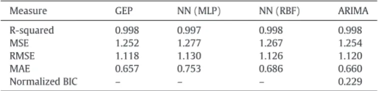
Measure GEP NN (MLP) NN (RBF) ARIMA

R-squared 0.998 0.997 0.998 0.998 MSE 1.252 1.277 1.267 1.254 RMSE 1.118 1.130 1.126 1.120 MAE 0.657 0.753 0.686 0.660 Normalized BIC – – – 0.229 Note:

MSE = mean squared error. RMSE = root mean squared error. MAE = mean absolute error. BIC = Bayesian information criterion.

0 1 2 3 4 5 2500 2600 2700 2800 2900 3000

BIC and Residual Sum of Squares

Number of breakpoints BIC RSS 50000 100000 150000 200000 250000

Fig. 13.Oil price series strructural breaks using BIC and RSS methods.

49

(11)

whereφ1,φ2…,φpθ1,θ2,…,θqare the unknown coefﬁcients to be

esti-mated using the maximum likelihood procedure.

∇d

¼ð1−BÞd ð5Þ

is a backward shift operator of order p deﬁned as:

∇zt¼zt–zt−1 with ∇d¼∇∇d−1 ð6Þ

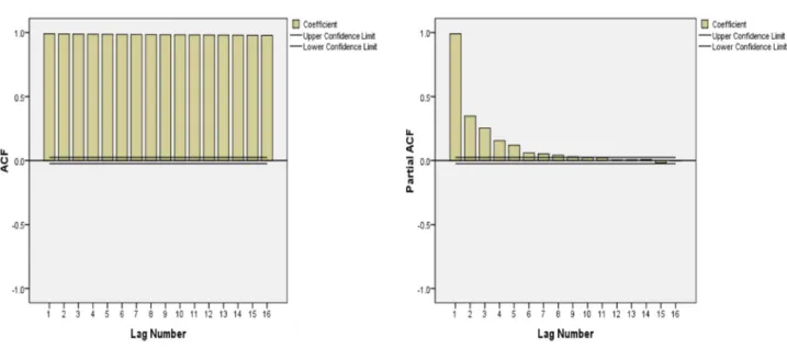
In this study we used both R version 3.0 and SPSS (PASW) version 20.0 packages to perform the three consecutive steps in ARIMA: identi-fication of the model, coefficients estimation and model verification. The ACF and PACF for the original series inFig. 11clearly shows that differencing is needed. A difference of order 1 stabilizes the series as shown inFig. 12. Thus an ARIMA with one difference is needed. After several model specifications, the best ARIMA model tofit our data was the ARIMA (0,1,5) model. This model has the lowest error rates and

the highest explanatory power out of all the other ARIMA models. This was conﬁrmed using the time series expert modeling function in SPSS (PASW) version 20.0. The Augmented Dickey–Fuller test (ADF) showed that the series was not stationary (Dickey–Fuller =−8, Lag order = 6, p-value = 0.01).Table 2shows the performance of the ARIMA model selected along with the NN and GEP models used in this study. From this table it is clear that the GEP model outperforms the NN and the ARIMA models in terms of several performance statistics such as the mean squared error, the root mean squared error, and the mean absolute error. The GEP model also has the highest explanatory power as measured by the R-squared statistic.

SinceNarayan and Liu's (2011)pioneering work,Salisu and Fasanya (2013) found that oil price series are generally characterized by structural breaks, we also model structural breaks using a monthly data series for the same period (January 1986 to June 2012). We used a monthly data set to model structural breaks in order to check the robustness of ourfindings. Narayan and Liu found two structural breaks in 1990 and 2008. The authors reported that thefirst break corresponds to the Kuwaiti–Iraqi war, while the second break corresponds to the financial crisis of 2008. Thus, the authors argued that there is some evidence of leverage effect in the volatility of oil price. In our study, both BIC and RSS methods detected three structural breaks in oil price series. The three breaks correspond to the invasion of Kuwait (1990) in which oil price increased to $33, the Asianfinancial crisis (1997) in which oil price decreased to $10, and the speculative behavior during the world-widefinancial crisis (2008) in which oil price increased to $145, respectively.Fig. 13shows the three breaks detected by the Bayesian Information Criterion and the Residual Sum of Squares methods. Formal tests confirmed the existence of three breaks

(F-0.0 0.5 1.0 1.5 2.0 0. 0 0. 6 Lag AC F 2 4 6 8 10 0. 0 0. 4 0. 8

p values for Ljung-Box statistic

lag

p

val

ue

Fig. 14.Fitted ARIMA model diagnostics.

Table 3

The ARIMA 95% CIs for the 6 months oil price forecast.

Mmonth Point forecast Lower limit Upper limit

July 2012 82.3 68.15 96.50 August 2012 82.3 62.25 102.40 September 2012 82.3 57.70 106.90 October 2012 82.3 53.84 110.80 November 2012 82.3 50.42 114.20 December 2102 82.3 47.31 117.30

(12)

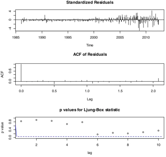
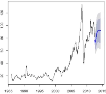
statistic: 630 on 3 and 314 df, p-valueb0.001).Fig. 14shows thefitted ARIMA model diagnostics. Based on standardized residuals, the resid-uals' ACF, and the Ljung–Box test, the model seems tofit the data well. Since both daily and monthly oil series data yield virtually the same re-sults, we report the 6-month ahead forecasts inTable 3.Fig. 15also re-ports the 80% and the 95% CIs for the next 24 months (out-of-sample forecast accuracy measures: RMSE = 3.61, MAE = 2.43, MPE =−1.16, MAPE = 6.67, MASE =−0.245). Finally, in this study we controlled for oil price psychological barrier effect in the oil market. FollowingAggarwal and Lucey (2007), we investigated whether the ab-normal distribution of oil prices occur when the prices are near barrier points by focusing on price movements along $10 barrier regions.De Zwart et al. (2009)found that traders usually shift to fundamental pric-ing models when markets are strongly dominated by fundamentals (as in the case during the 2007–2012 oil market), leaving virtually no room for psychological barriers' influence. Thus, we tested for psychological barriers by splitting our data into two periods: 1986–2006 and 2007– 2012. This split is based onDe Zwart et al. (2009)theoreticalfindings. It is also based on the fact that we can practically capture both the peak in oil prices in 2007 ($146 per barrel) and the collapse of oil price during the 2008 worldwide credit crisis. Three formal tests were employed to check for price clusters/psychological barrier based on the frequency of oil price over the two samples based on the last digit. The tests are the standardX2_goodness-of-_fi_{t test, the Hirshmann}_– Herfindal Index (HHI), and the Standardized Range (SR) test. All tests have straightforward interpretation. For example, in the SR test the market with a higher estimated standardized range value would indicate a higher degree of price clustering/psychological barrier. The results of the tests seem to indicate that psychological barriers appear to influence oil prices only in the range 1986–2006 (the period before the credit crisis). This result seems to confirm the theoreticalfindings ofDe Zwart et al. (2009).

As reported in the previous paragraph, we have checked our results for robustness by modeling both daily and monthly time series of oil price. However, it should be noted that previous research has used different forms of time series in theﬁeld of oil price modeling. For exam-ple,Phan et al. (2015c)used a 5-minute time frame. Studies byNarayan and Narayan (2010);Narayan et al. (2010);Narayan et al. (2011);

Narayan and Sharma (2011)andNarayan and Sharma (2014);Kang et al. (2015)andPhan et al. (2015a), used daily data.Driesprong et al. (2008); Nandha and Faff (2008)andNarayan and Gupta (2015)used

monthly data.Narayan et al. (2014)used quarterly data. Yet,Prasad et al. (2007)used annual data.

5. Conclusions, limitations and future research

Crude oil plays an increasingly important role in world economy. We applied evolutionary techniques such as GEP and NN models to predict oil prices. ARIMA models are employed to benchmark evolutionary models. The results reveal that the GEP technique outperforms traditional statistical techniques in predicting oil prices. The GEP model nearly perfectly predicts oil price in the study period. These results of this study have several important implications. Superior performance of evolutionary techniques found in this study conﬁrms the theoreticalﬁndings ofHecht-Nielson (1989)andHaykin (2001)

who have shown that NN and genetic algorithms' techniques can make perfect predictions. Our results also corroborate theﬁndings of other researchers who have investigated the performance of NN and GEP techniques compared to other traditional statistical techniques, such as regression analysis, discriminant analysis, and logistic regres-sion. For example,Shan et al. (2002)found a hit ratio of 85% for the PNN model compared to 80% for the LDA model in a study of clinical diagnosis of cancers.Bensic et al. (2005)compared the performance of logistic regression, neural networks and decision trees in a study of credit-scoring models. The authors found that the PNN model produced the highest hit rate and the lowest type I error.Ravi et al. (2007)

compared statistical and NN techniques on a data profiling Internet banking users in India. Their results showed that NN models achieved 100% overall accuracies for the test data.Koh (2004)investigated the going concern prediction using machine learning techniques. The author reported superior results for NN models. Finally,Kiang and Kumar (2001)found that NN models and genetic algorithms techniques provide more accurate forecasting for simulated data when input data are skewed. Despite our promising results, this study suffers from a number of limitations. First, this study has used a longitudinal approach representing a time series oil price data from 1986 to 2012. Future research might want to test whether our results hold taking into consid-eration the influence of several economic and political issues. It should also be noted that for the purpose of this research, GEP and NN approaches were adopted to predict oil prices. Although the use of quantitative methods is valuable in establishing relationships between variables, these approaches are considered weak when trying to deter-mine the reasons behind such relationships. Quantitative methods are used for the purpose of utilizing variables that have an impact on oil prices and can be taken into consideration for further segmentation; which can be either non-standard or econometric models. In light of the importance of crude oil to the world's economy, it is not sur-prising that economists have devoted great efforts towards develop-ing methods to forecast price and volatility levels. While the most popular forecasting approaches are based on traditional economet-rics, computational approaches such as artificial neural networks and fuzzy expert systems have gained popularity infinancial mar-kets because of theirflexibility and accuracy. However, there is still no general consensus on which methods are more reliable Thus, fu-ture research might use a mixed quantitative–qualitative approach to investigate the dynamic determinants of oil prices in global mar-kets. Finally, we applied GEP and NN models successfully to forecast oil price across a long time series. Although we expect such algo-rithms to work also in forecasting other commodities such as gold and precious metal (Chiroma et al., 2013; Jianhui and Wei, 2012; Castillo and Melin, 2002), future research may test whether this holds across different domains.

Acknowledgment

The authors would like to thank an anonymous referee and the edi-tor for insightful comments on a previous version of this paper.

Fig. 15.ARIMA model forecasts (July 2012–June 2014).

51

(13)

Int. J. Prod. Econ. 134, 463–471.

Balasubramanian, M., Palanivel, S., Rmalingam, V., 2009.Real time face and mouth recognition using radial basis function neural networks. Expert Syst. Appl. 36, 6879–6888.

Baykasoĝlu, A., Göçken, M., 2009.Gene expression programming based due date assign-ment in a simulated job shop. Expert Syst. Appl. 36, 12143–12150.

Bensic, M., Sarlija, N., Zekic-Susac, M., 2005.Modelling small-business credit scoring by using logistic regression, neural networks and decision trees. Intel. Sys. Account. Fin. Manag. 13, 133–150.

Bishop, C., 2006.Pattern Recognition and Machine Learning. second ed. Springer, New York.

Calderon, T., Cheh, J., 2002.A roadmap for future neural networks research in auditing and risk assessment. Int. J. Account. Inf. Syst. 3, 203–236.

Castillo, O., Melin, P., 2002.Hybrid intelligent systems for time series prediction using neural networks, fuzzy logic, and fractal theory. IEEE Trans. Neural Netw. 13, 1395–1408.

Celikoglu, H., Cigizoglu, H., 2007.Modelling public transport trips by radial basis function neural networks. Math. Comput. Model. 45, 480–489.

Chen, S., 2002.Genetic Algorithms and Genetic Programming in Computational Finance. Kluwer Academic Publishers, Amsterdam.

Chen, M., Huang, S., 2003.Credit scoring and rejected instances reassigning through evo-lutionary computation techniques. Expert Syst. Appl. 24, 433–441.

Cheng, C., Chen, C., Fu, C., 2006.Financial distress prediction by radial basis function net-work with logit analysis learning. Comput. Math. Appl. 51, 579–588.

Chiroma, H., Abdulkareem, S., Abubakar, A., Zeki, A., Gital, A.Y., 2013.Intelligent system for predicting the price of natural gas based on non-oil commodities. IEEE Symposium on Industrial Electronics & Applications ISIEA2013, September 22–25, Kuching, Malaysia. Christodoulos, C., Michalakelis, C., Varoutas, D., 2010.Forecasting with limited data:

com-bining ARIMA and diffusion models. Technol. Forecast. Soc. Chang. 77, 558–565. Ciner, C., 2001.Energy shocks andﬁnancial markets: nonlinear linkages. Stud. Nonlinear

Dynam. Econometrics 5 (3), 203–212.

Darbellay, G., Slama, M., 2000.Forecasting the short-term demand for electricity: do neu-ral networks stand a better chance? Int. J. Forecast. 16, 71–83.

De Zwart, G., Markwat, T., Swinkels, L., van Dijik, D., 2009.The economic value of funda-mental and technical information in emerging currency markets. J. Int. Money Financ. 28 (4), 581–604.

Dehuri, S., Cho, S.B., 2008.Classiﬁcation rule mining using gene expression programming. Third International Conference on Convergence and Hybrid Informat 2, pp. 754–760. Dhanalakshmi, P., Palanivel, S., Ramalingam, V., 2009.Classiﬁcation of audio signals using

SVM and RBFNN. Expert Syst. Appl. 36, 6069–6075.

Dowling, M., Cummins, M., Lucey, B.M., 2014.Psychological barriers in oil futures markets. Energy Econ. xxx (xxx–xxx).

Driesprong, G., Jacobsen, B., Maat, B., 2008.Striking oil: another puzzle? J. Financ. Econ. 892, 307–327.

Ediger, V., Akar, S., Ugurlu, B., 2006.Forecasting production of fossil fuel sources in Turkey using a comparative regression and ARIMA model. Energ Policy 34, 3836–3846. Fan, Y., Liang, Q., Wei, Y.-M., 2008.A generalized pattern matching approach for

multi-step prediction of crude oil price. Energy Econ. 30, 889–904.

Ferreira, C., 2001.Gene expression programming: a new adaptive algorithm for solving problems. Complex Sys. 13, 87–129.

Ferreira, C., 2004.Gene expression programming and the evolution of computer pro-grams. In: de Castro, L.N., Von Zuben, F.J. (Eds.), Recent Developments in Biologically Inspired Computing. Idea Group Publishing, pp. 82–103.

Ferreira, C., 2006.Gene Expression Programming: Mathematical Modelling by an Artiﬁcial Intelligence. Springer, San Francisco.

Gao, J., Hu, J., Mao, X., Perc, M., 2012. Culturomics meets random fractal theory: insights into long-range correlations of social and natural phenomena over the past two cen-turies. J. R. Soc. Interface 1–9.http://dx.doi.org/10.1098/rsif.2011.0846.

Ghaffari, A., Zare, S., 2009.A novel algorithm for prediction of crude oil price variation-based on soft computing. Energy Econ. 31, 531–536.

Gisser, M., Goodwin, T.H., 1986.Crude oil and the macroeconomy: tests of some popular notions. J. Money, Credit, Bank. 18 (1), 95–103.

Gorr, W., Nagin, D., Szczypula, J., 1994.Comparative study of artiﬁcial neural network and statistical models for predicting student point averages. Int. J. Forecast. 10, 17–34. Gupta, K.R., Bhunia, A.K., Goyal, S.K., 2007.An application of genetic algorithm in a

mar-keting oriented inventory model with interval valued inventory costs and three-component demand rate dependent on displayed stock level. Appl. Math. Comput. 192, 466–478.

J. Monet. Econ. 38, 195–213.

Hosseini, S., Gandomi, A., 2012.Short-term load forecasting of power systems by gene expression programming. Neural Comput. & Applic. 21, 377–389.

Hung, R.D., Masulis, R.W., Stoll, H.R., 1996.Energy shocks andﬁnancial markets. J. Futur. Mark. 16, 1–27.

Iyer, S., Sharda, R., 2009.Prediction of athletes' performance using neural networks: an application in cricket team selection. Expert Syst. Appl. 36, 5510–5522.

Jammazi, R., Aloui, C., 2012.Crude oil price forecasting: experimental evidence from wavelet decomposition and neural network modelling. Energy Econ. 34, 828–841. Jiang, E., 2007.Detecting spam email by radial basis function networks. Int. J. Know.-based

Eng. Sys. 11, 409–418.

Jianhui, Y., Wei, D., 2012. Prediction of Gold price based on WT-SVR and EMD-SVR model. Eighth International Conference on Computational Intelligence and Security, 17–18 Nov. 2012, Guangzhou, China, 415–419. http://dx.doi.org/10.1109/CIS.2012.99. Jones, C.M., Kaul, G., 1996.Oil and the stock markets, J. Finance 51 (2), 463–491. Kadkhodaie-Ilkhchi, A., Rezaee, M., Rahimpour-Bonab, H., 2009.A committee neural

net-work for prediction of normalized oil content from well log data: an example from South Pars Gas Field, Persian Gulf. J. Pet. Sci. Eng. 65, 23–32.

Kahyaoglu, T., 2008.Optimization of the pistachio nut roasting process using response surface methodology and gene expression programming. LWT Food Sci. Technol. 41, 26–33.

Kang, W., Ratti, R.A., Yoon, K.H., 2015.The impact of oil price shocks on the stock market return and volatility relationship. J. Int. Financ. Mark. Inst. Money 34, 41–54. Kiang, M., Kumar, A., 2001.An evaluation of self-organizing map network as a robust

al-ternative to factor analysis in data mining applications. Inf. Syst. Res. 12, 177–194. Kodba, S., Perc, M., Marh, M., 2005.Detecting chaos from a time series. Eur. J. Phys. 26,

205–215.

Koh, H., 2004.Going concern prediction using data mining techniques. Manag. Audit. J. 19, 462–476.

Kohzadi, N., Boyd, M., Kemlanshahi, B., Kaastra, I., 1996.A Comparison of artiﬁcial neural network and time series models for forecasting commodity prices. Neurocomputing 10, 169–181.

Kostic, S., Perc, M., Vasovic, N., Trajkovic, S., 2013.Predictions of experimentally observed stochastic ground vibrations induced by blasting. PLoS ONE 8, 1–13.

Koutroumanidis, T., Ioannou, K., Arabatzis, G., 2009.Predicting fuelwood prices in Greece with the use of ARIMA models, artiﬁcial neural networks and a hybrid ARIMA–ANN model. Energ Policy 37, 3627–3634.

Kumar, K., Bhattacharya, S., 2006.Artiﬁcial neural network vs. linear discriminant analysis in credit ratings forecast. Rev. Account. Financ. 5, 216–227.

Lapedes, A., Farber, R., 1988.How neural nets work? In: Anderson, D. (Ed.), Neural Infor-mation Processing Systems, A. Instit of Physics, pp. 442–456 (New York) Lek, S., Guegan, J., 1999.Artiﬁcial neural networks as a tool in ecological modelling: an

in-troduction. Ecol. Model. 120, 65–73.

Li, Q., Cai, Z., Jiang, S., Zhu, L., 2004.Gene expression programming in prediction. Proceed-ings of the 5th World Congress on Intelligent Control and Automation, 3, 2171–2175, June 15–19, Hangzhou, P.R. China.

Lim, C., Kirikoshi, T., 2005.Predicting the effects of physician-directed promotion on pre-scription yield and sales uptake using neural networks. J. Target. Meas. Anal. Mark. 13, 158–167.

Lisboa, P., Vellido, A., 2000.Business applications of neural networks. In: Lisboa, P., Edisbury, B., Vellido, A. (Eds.), Business Applications of Neural Networks: The State-of-the-art of Real-world Applications. World Scientiﬁc, Singapore, pp. vii–xxii. Liu, H., Wen, Y., Gao, Y., 2009.Application of experimental design and radial basis function

neural network to the separation and determination of active components in tradi-tional Chinese medicines by capillary electrophoresis. Anal. Chim. Acta 638, 88–93. Lopez, H., Weinert, W., 2004a.EGIPSYS: an enhanced gene expression programming

ap-proach for symbolic regression problems. Int. J. Appl. Math. Comput. Sci. 14, 375–384. Lopez, S., Weinert, R., 2004b.An enhanced gene expression programming approach for

symbolic regression problems. Int. J. Appl. Math. Comput. Sci. 14, 375–384. Margny, M.H., El-Semman, I.E., 2005.Extracting logical classiﬁcation rules with

expres-sion programming: micro array case study. Conference Proceedings, AIML 05, Cairo, Egypt.

McMenamin, J., Monforte, F., 1998.Short-term energy forecasting with neural networks. Energy J. 19, 43–52.

Mingming, T., Jinliang, Z., 2012.A multiple adaptive wavelet recurrent neural network model to analyze crude oil prices. J. Econ. Bus. 64, 275–286.

Mohammadi, H., Su, L., 2010.International evidence on crude oil price dynamics: applica-tions of ARIMA–GARCH models. Energy Econ. 32, 1001–1008.

(14)

Mostafa, M., 2004.Forecasting the Suez Canal trafﬁc: a neural network analysis. Marit. Policy Manag. 31, 139–156.

Nam, K., Yi, J., 1997.Predicting airline passenger volume. J. Bus. Forecast. Methods Sys. 16, 14–17.

Nandha, M., Faff, R., 2008.Does oil move equity prices? A global view. Energy Econ. 30, 986–997.

Narayan, P.K., Gupta, R., 2015.How oil price predicted stock returns for over a century? Energy Econ. 48, 18–23.

Narayan, P.K., Liu, R., 2011.Are shocks to commodity prices persistent? Appl. Energy 88, 409–416.

Narayan, P.K., Narayan, S., 2010.Modelling the impact of oil prices on Vietnam's stock prices. Appl. Energy 87 (1), 356–361.

Narayan, P.K., Narayan, S., 2014. Psychological oil price barrier andﬁrm returns. J. Behav. Financ. 15 (4), 318–333.http://dx.doi.org/10.1080/15427560.2014.968719. Narayan, P.K., Sharma, S.S., 2011.New evidence on oil price andﬁrm returns. J. Bank.

Financ. 35, 3253–3262.

Narayan, P.K., Sharma, S.S., 2014.Firm return volatility and economic gains: the role of oil prices. Econ. Model. 38, 142–151.

Narayan, P.K., Narayan, S., Popp, S., 2010.A note on the long-run elasticities from the en-ergy consumption–GDP relationship. Appl. Enen-ergy 87 (3), 1054–1057.

Narayan, P.K., Narayan, S., Popp, S., D'Rosario, M., 2011.Share price clustering in Mexico. Int. Rev. Financ. Anal. 20 (2), 113–119.

Narayan, P.K., Sharma, S., Poon, W.C., Westerlund, J., 2014.Do oil prices predict economic growth? New global evidence. Energy Econ. 41 (2014), 137–146.

Nazari, A., 2012.Prediction performance of PEM fuel cells by gene expression program-ming. Int. J. Hydrog. Energy 37, 18972–18980.

Nazari, A., Riahi, S., 2012. Predicting the effects of nanoparticles on compressive strength of ash-based geopolymers by gene expression programming. Neural Comput. & Applic.http://dx.doi.org/10.1007/s00521-012-1127-7.

Papapetrou, E., 2001.Oil price shocks, stock market, economic activity and employment in Greece. Energy Econ. 23 (5), 511–532.

Paz-Marín, M., Campoy-Muñoz, P., Hervás-Martínez, C., 2012.Non-linear multiclassiﬁer model based on artiﬁcial intelligence to predict research and development perfor-mance in European countries. Technol. Forecast. Soc. Chang. 79, 1731–1745. Phan, D.H.B., Sharma, S.S., Narayan, P.K., 2015a.Oil price and stock returns of consumers

and producers of crude oil. J. Int. Financ. Mark. Inst. Money 34, 245–262. Phan, D.H.B., Sharma, S.S., Narayan, P.K., 2015b.Stock return forecasting: some new

evi-dence. Int. Rev. Financ. Anal. 40, 38–51.

Phan, D.H.B., Sharma, S.S., Narayan, P.K., 2015c. Intraday volatility interaction between the crude oil and equity markets. J. Int. Financ. Mark. Inst. Money. http://dx.doi.org/10. 1016/j.intﬁn.2015.07.007(xx, xxx–xxx).

Poh, H., Yao, J., Jasic, T., 1998.Neural networks for the analysis and forecasting of adver-tising impact. Int. J. Intellig. Sys. Account. Financ. Manag. 7, 253–268.

Pradhan, R.P., Arvin, M.B., Ghoshray, A., 2015.The dynamics of economic growth, oil prices, stock market depth, and other macroeconomic variables: evidence from the G-20 countries. Int. Rev. Financ. Anal. 39, 84–95.

Prasad, A., Narayan, P.K., Narayan, J., 2007.Exploring the oil price and real GDP nexus for a small island economy, the Fiji Islands. Energ Policy 35 (12), 6506–6513.

Ravi, V., Carr, M., Sagar, N., 2007.Proﬁling of Internet banking users in India using intelli-gent techniques. J. Serv. Res. 6, 61–73.

Reddy, M., Ghimire, B., 2009.Use of model tree and gene expression programming to predict the suspended sediment load in rivers. J. Intell. Syst. 18, 211–228.

Ruiz-Suarez, J., Mayora-Ibarra, O., Torres-Jimenez, J., Ruiz-Suarez, L., 1995.Short-term ozone forecasting by artiﬁcial neural network. Adv. Eng. Softw. 23, 143–149. Ryan, N., Hibler, D., 2011.Robust gene expression programming, procedia comput.

Sci-ence 6, 165–170.

Salisu, A.A., Fasanya, I.O., 2013.Modelling oil price volatility with structural breaks. Energ Policy 52, 554–562.

Sermpinis, G., Laws, J., Karathanasopoulos, A., Dunis, C.L., 2012.Forecasting and trading the EUR/USD exchange rate with gene expression and Psi sigma neural networks. Ex-pert Syst. Appl. 39, 8865–8877.

Shambora, W., Rossiter, R., 2007.Are there exploitable inefﬁciencies in the futures market for oil? Energy Econ. 29, 18–27.

Shan, Y., Zhao, R., Xu, G., Liebich, H.M., Zhang, Y., 2002.Application of probabilistic neural network in the clinical diagnosis of cancers based on clinical chemistry data. Anal. Chim. Acta 471, 77–86.

Sharda, R., 1994.Neural networks for the MS/OR analyst: an application bibliography. In-terfaces 24, 116–130.

Spear, N., Leis, M., 1997.Artiﬁcial neural networks and the accounting method choice in the oil and gas industry. Account. Manag. Inf. Technol. 7, 169–181.

Stevens, P., 1995.The determination of oil prices 1945–1995. Energ Policy 23, 861–870. Swicegood, P., Clark, J., 2001. Off-site monitoring systems for prediction bank

underperformance: a comparison of neural networks, discriminant analysis, and pro-fessional human judgment. Int. J. Intellig. Sys. Account. Financ. Manag. 10, 169–186. Teodorescu, I., 2006.Gene expression programming approach to event selection in high

energy physics. IEEE Trans. Nucl. Sci. 53, 2221–2227.

Teodorescu, L., Sherwood, D., 2008.High energy physics event selection with gene ex-pression programming. Comput. Phys. Commun. 178, 409–419.

Terzi, O., 2012. Daily pan evaporation estimation using gene expression programming and adaptive neural-based fuzzy inference system. Neural Comput. & Applic.http:// dx.doi.org/10.1007/s00521-012-1027-x.

Tseng, F.-M., Yu, H.-C., Tzeng, G.-H., 2002.Combining neural network model with seasonal time series ARIMA model. Technol. Forecast. Soc. Chang. 69, 71–87.

Verleger, P.K., 1993.Adjusting to Volatile Energy Prices. Institute for International Eco-nomics, Washington DC.

Videnova, I., Nedialkova, D., Dimitrova, M., Popova, S., 2006.Neural networks for air pol-lution forecasting. Appl. Artif. Intell. 20, 493–506.

Visoiu, A., 2011.Deriving trading rules using gene expression programming. Inf. Econ. 15, 22–30.

Wang, S., 1995.The unpredictability of standard back propagation neural networks in classiﬁcation applications. Manag. Sci. 41, 555–559.

Wang, S.Y., Yu, L., Lai, K.K., 2005.Crude oil price forecasting with TEI@I methodology. J. Syst. Sci. Complex. 18, 145–166.

Wang, W., Du, Y., Li, Q., Fang, Z., 2011.Credit evaluation based on gene expression programming and clonal selection. Procedia Eng. 15, 3759–3763.

Watkins, G.C., Plourde, A., 1994.How volatile are crude oil prices? OPEC Rev. 18, 220–245. Weigend, A.S., Gershenfeld, N.A., 1994.Time Series Prediction: Forecasting the Future and

Understanding the Past. Addison-Wesley, Reading, MA.

Xu, K., Liu, Y., Tang, R., Zuo, J., Tang, C., 2009.A novel method for real parameter optimi-zation based on gene expression programming. Appl. Soft Comput. 9, 725–737. Yu, L., Wang, S., Lai, K., 2008.Forecasting crude oil price with an EMD- based neural

network ensemble learning paradigm. Energy Econ. 305, 2623–2635.

Zhuo, W., Li-Min, J., Yong, Q., Yan-Hui, W., 2007.Railway passenger trafﬁc volume predic-tion based on neural network. Appl. Artif. Intell. 21, 1–10.

53