Virginia Commonwealth University Virginia Commonwealth University
VCU Scholars Compass
VCU Scholars Compass
Theses and Dissertations Graduate School
2017
Decomposition Algorithms in Stochastic Integer Programming:
Decomposition Algorithms in Stochastic Integer Programming:
Applications and Computations.
Applications and Computations.
Babak Saleck PayFollow this and additional works at: https://scholarscompass.vcu.edu/etd
Part of the Industrial Engineering Commons, Operational Research Commons, Other Operations Research, Systems Engineering and Industrial Engineering Commons, and the Systems Engineering Commons
© The Author
Downloaded from Downloaded from
https://scholarscompass.vcu.edu/etd/5027
c
Babak Saleck Pay, August 2017 All Rights Reserved.
i
DECOMPOSITION ALGORITHMS IN STOCHASTIC INTEGER PROGRAMMING: APPLICATIONS AND COMPUTATIONS.
A dissertation submitted in partial fulfillment of the requirements for the degree of Doctor of Philosophy (Systems Modeling and Analysis)
at Virginia Commonwealth University.
by
BABAK SALECK PAY
Director: Dr. Yongjia Song, Assistant Professor
Department of Statistical Sciences and Operations Research
Virginia Commonwealth University Richmond, Virginia
Acknowledgements
I would like to express my deepest gratitude to all people who helped me during this journey.
First, I really thank my dear family, Baba, Moman, Abji and Madar (RIP). They were a true supporters and were there whenever I needed help. There is a strong emotional bound among us which neither time nor distance can break.
Second, I want to thank my dear adviser Dr. Yongjia Song. During the four years of PhD, I have learned a lot from him, either in his classrooms or in our research meeting. He helped me generously in every aspect of this job.
I also want to thank Dr. Jason Merrick for trusting and granting me the PhD position.
I want to express my gratitude to the other members of my committee: Dr. J Paul Brooks, Dr. Jos´e Dul´a, and Dr. Qin Wang. They are great scholars in their communities and I am very proud to have this unique opportunity to work with them.
TABLE OF CONTENTS Chapter Page Acknowledgements . . . iii Table of Contents . . . iv List of Tables . . . vi List of Figures . . . ix Abstract . . . xi 1 Introduction . . . 1
1.1 Stochastic Linear/Integer Programming . . . 1
1.1.1 Benders decomposition . . . 6
1.1.2 Level decomposition . . . 8
1.1.3 Adaptive partition-based algorithms . . . 9
1.2 Expected Utility . . . 12
1.3 Network Interdiction Problem . . . 15
2 Stochastic Network Interdiction with Incomplete Preference . . . 21
2.1 Introduction . . . 21
2.2 Stochastic Shortest Path Interdiction with Incomplete Defender’s Preference . . . 23
2.2.1 Preliminaries: expected utility and incomplete preference . . 24
2.2.2 Fitting the utility function using piecewise linear concave functions . . . 27
2.3 Robust expected utility framework with incomplete preference . . . 32
2.3.1 A robust utility model for stochastic shortest path inter-diction with incomplete defender’s preference . . . 35 2.3.2 A robust certainty equivalent model for stochastic
2.4 Computational Experiments . . . 40
2.4.1 Instance generation . . . 40
2.4.2 Computational settings . . . 41
2.4.3 Comparison between the robust expected utility model and the robust certainty equivalent model . . . 42
2.4.4 Comparison between the robust expected utility model and the best fitted piecewise linear concave utility model . . 45
2.4.5 Computational performances . . . 50
2.4.6 Summary of computational experiments . . . 53
2.5 Extensions . . . 54
2.6 Concluding Remarks . . . 57
3 Partition-based Decomposition Algorithms for Two-stage Stochastic Integer Programs with Continuous Recourse . . . 59
3.1 Introduction . . . 59
3.2 Partition-Based Decomposition Algorithms for Two-Stage Stochas-tic Integer Programs with Continuous Recourse . . . 60
3.2.1 A partition-based branch-and-cut algorithm . . . 61
3.2.2 Stabilizing the partition-based decomposition algorithm . . . 66
3.3 Computational Experiments . . . 69
3.3.1 Computational setup . . . 70
3.3.2 Implementation details . . . 71
3.3.3 Heuristic refinement strategies . . . 79
3.4 Conclusion . . . 84
4 Partition-based Dual Decomposition for Two-stage Stochastic Integer Programs with Integer Recourse . . . 86
4.1 Introduction . . . 86
4.2 Problem Setting and Background . . . 90
4.2.1 Dual Decomposition . . . 91
4.2.2 Dual Decomposition with Scenario Grouping . . . 96
4.2.3 Partition-based Dual Decomposition . . . 97
4.3 Partition-based Relaxation Strategies for SIP . . . 101
4.3.1 Strategy 1: One-phase PDD . . . 102
4.4 Computational Experiments . . . 105
4.4.1 Computational Setting . . . 106
4.4.2 Numerical Results . . . 106
LIST OF TABLES
Table Page
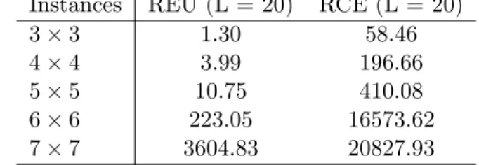
1 Comparison of the solution behavior for the risk neutrial model (RNM), robust expected utility model (REU) with 20 and 3 pairwise compar-isons, and robust certainty equivalent model (RCE) with 3 pairwise
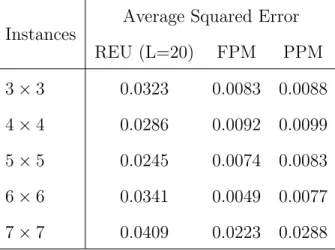
gamble comparisons using CVaR. . . 44 2 Comparison of solution time for REU and RCE with L= 20 . . . 44 3 The average squared error between the resulting utility function from
each model (REU, FPM and PPM) and the true utility function. All
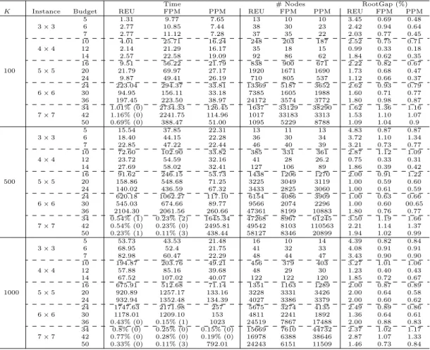
instances considered in this table have 100 scenarios and budget ratio 0.4. 47 4 Average computational time (including the time spent on fitting the
utility function for approach FPM and PPM), number of nodes ex-plored in the branch-and-bound tree, and the root optimality gap for three approaches REU, FPM and PPM for grid network instances
with various network sizes, interdiction budgets, and scenario sizes. . . 51 5 Average computational time for two approaches, REU and PPM, on
sets of pairwise gamble comparisons of different sizes (20, 50, and 100,
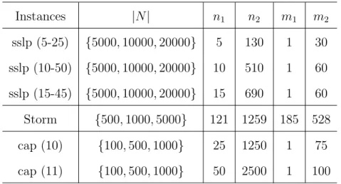
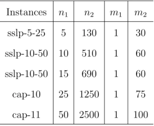
respectively). . . 52 6 Profiles of test instances (|N|is the number of scenarios,n1andm1are
the numbers of first-stage variables and constraints, respectively, and n2 andm2 are the numbers of second-stage variables and constraints,
respectively). . . 70 7 Computational results for algorithms “Extensive”, “Benders” and “Level”. 74 8 Computational results for three variants of the adaptive
partition-based decomposition algorithms, B&C” (Algorithm 2), “Partition-Naive” and “Partition-Level” (Algorithm 3). . . 75
9 Number of cuts (coarse and fine) and the final partition size for three variants of the adaptive partition-based decomposition algorithms, B&C” (Algorithm 2), Naive” and
“Partition-Level” (Algorithm 3). . . 76 10 Computational result comparisons between full refinement and partial
refinement strategies for variant “Partition-B&C”. . . 77 11 Computational results for algorithm “Partition-B&C” using a
heuris-tic refinement strategy. . . 82 12 Computational results for algorithm “Partition-Level” using a
heuris-tic refinement strategy. . . 83 13 Profile of instances (n1andn2 are number of variables in the first-stage
and second-stage;m1 and m2 are number of constraints in first-stage
and second-stage) . . . 105 14 Numerical results (lower bound and number of iterations) for class
easy instances to compare One-phase PDD versus DD.. . . 108 15 Numerical results (lower bound and number of iterations) for class
hard instances to compare One-phase PDD versus DD. . . 109 16 Computational time for Two-phase PDD versus GDD . . . 112 17 Comparison of lower bound for Two-phase PDD versus GDD for class
hard . . . 113 18 Comoputational time for Two-phase PDD versus GDD for class hard. . . 113 19 Full computational results for three approaches REU, FPM and PPM
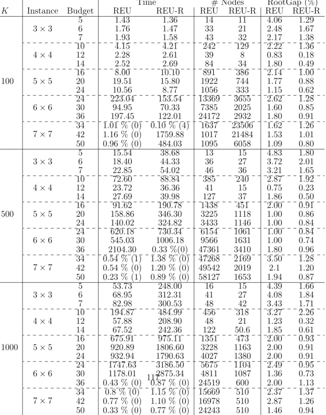
on instances with different interdiction budget ratios (0.4, 0.5, and 0.6). . 116 20 Full computational results for two formulation REU and REU-R on
21 Computational time (in seconds) for two approaches, REU and PPM, with 20, 50, and 100 pairwise gamble comparisons, using different
interdiction budget ratios (0.4, 0.5, and 0.6). . . 118 22 Detailed time profile (in seconds) for the three phases involved in
approach PPM: computing the upper bound ¯uj and lower bound uj for j ∈ T (Bound), fitting the piecewise linear concave function with a fixed number of pieces (Fitting), and optimize the expected utility
LIST OF FIGURES
Figure Page
1 Illustration on the tail distributions of the optimal solutions obtained by model RNM, REU withL = 3 and L = 20, and RCE with L= 3
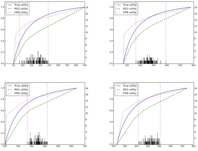
for a 3×3 grid network instance with 100 scenarios and budget ratio 0.4. 46 2 An illustration of the true utility function, the worst-case utility
func-tion resulting from the REU model, and the fitted utility funcfunc-tion from the FPM model for four grid network instances: 3×3 with interdic-tion budget r0 = 6 (top left), 4×4 with interdiction budget r0 = 10
(top right), 5×5 with interdiction budget r0 = 16 (bottom left) and
6×6 with r0 = 34 (bottom right) with 100 scenarios and 20 pairwise
Abstract
DECOMPOSITION ALGORITHMS IN STOCHASTIC INTEGER PROGRAMMING: APPLICATIONS AND COMPUTATIONS.
By Babak Saleck Pay
A dissertation submitted in partial fulfillment of the requirements for the degree of Doctor of Philosophy at Virginia Commonwealth University.
Virginia Commonwealth University, 2017.
Director: Dr. Yongjia Song, Assistant Professor Department of Statistical Sciences and Operations Research
In this dissertation we focus on two main topics. Under the first topic, we develop a new framework for stochastic network interdiction problem to address ambiguity in the defender risk preferences. The second topic is dedicated to com-putational studies of two-stage stochastic integer programs. More specifically, we consider two cases. First, we develop some solution methods for two-stage stochastic integer programs with continuous recourse; second, we study some computational strategies for two-stage stochastic integer programs with integer recourse.
We study a class of stochastic network interdiction problems where the defender has incomplete (ambiguous) preferences. Specifically, we focus on the shortest path network interdiction modeled as a Stackelberg game, where the defender (leader) makes an interdiction decision first, then the attacker (follower) selects a shortest
path after the observation of random arc costs and interdiction effects in the net-work. We take a decision-analytic perspective in addressing probabilistic risk over network parameters, assuming that the defender’s risk preferences over exogenously given probabilities can be summarized by the expected utility theory. Although the exact form of the utility function is ambiguous to the defender, we assume that a set of historical data on some pairwise comparisons made by the defender is available, which can be used to restrict the shape of the utility function. We use two different approaches to tackle this problem. The first approach conducts utility estimation and optimization separately, by first finding the best fit for a piecewise linear concave utility function according to the available data, and then optimizing the expected utility. The second approach integrates utility estimation and optimization, by mod-eling the utility ambiguity under a robust optimization framework following [4] and [44]. We conduct extensive computational experiments to evaluate the performances of these approaches on the stochastic shortest path network interdiction problem.
In third chapter, we propose partition-based decomposition algorithms for solv-ing two-stage stochastic integer program with continuous recourse. The partition-based decomposition method enhance the classical decomposition methods (such as Benders decomposition) by utilizing the inexact cuts (coarse cuts) induced by a sce-nario partition. Coarse cut generation can be much less expensive than the standard Benders cuts, when the partition size is relatively small compared to the total num-ber of scenarios. We conduct an extensive computational study to illustrate the advantage of the proposed partition-based decomposition algorithms compared with the state-of-the-art approaches.
In chapter four, we concentrate on computational methods for two-stage stochas-tic integer program with integer recourse. We consider the partition-based relaxation framework integrated with a scenario decomposition algorithm in order to develop strategies which provide a better lower bound on the optimal objective value, within a tight time limit.
CHAPTER 1
INTRODUCTION
1.1 Stochastic Linear/Integer Programming
Stochastic programming has firmly established itself as an indispensible modeling tool and solution approach to deal with optimization problems under uncertainty [10]. Among all the stochastic programming models, two-stage stochastic program is one of the most popular models that has been applied in a variety of application areas, see, e.g., [46, 21, 11, 101, 75, 102, 3]. In two-stage stochastic programs, the first-stage decisions, known as the here-and-now decisions, are made before the realization of the random parameters in the model. On the other hand, the second-stage decisions, known as the wait-and-see decisions, are made after resolutions of the random pa-rameters are observed. The second-stage decisions are meant to compensate for the first-stage decisions, and therefore are also called therecourse decisions.
We present a two-stage stochastic linear program as follows:
z∗ = min x∈X c
Tx+
where
f(x, ξ) = mindTy (1.2a)
s.t. ˜T x+W y≥˜h (1.2b)
y ∈Rn2. (1.2c)
In (1.1), X ⊂ Rn1 is a non-empty and closed set. In (1.2), the triple (Ω,F,P) is a probability space in whichξ= ( ˜T ,˜h) is defined and the closed set Ξ⊂RD is the support forP.
There are two basic assumptions upon which most of the methods in stochastic programming are built. The first assumption is that the probability distribution of ξ is known; but, in most cases, calculating the expected value E[f(x, ξ)] is compu-tationally very intensive. Moreover, if decision maker accept a good approximate solution, then we might be able to avoid this intense calculation. Hence, we can follow the most common procedure in stochastic programming which is finding a discrete set of realization of random parameters. This set is used to approximate the true underlying probability distribution. The larger the set, the better the ap-proximation. In stochastic programming literature, we call the set defined above as scenario set and the problems that use such a set are called scenario-based problems. The second assumption is the independence of random parametersξ of decision vari-able x. See [35] for a class of problems that violate this assumption. Throughout this dissertation, we follow these two assumptions.
Given a set of independent random samples ξ1, ξ2,· · ·ξN, we have:
fN(x) =
PN
k=1fk(x)
|N| , (1.3)
where for each scenario k ∈ N, fk(x) represents the second-stage value function, which is given by:
fk(x) := min yk∈
Rn+2
d>yk | Tkx+W yk ≥hk . (1.4)
Note thatN ={1,2, . . . , N}is the the set of indices corresponding to each scenario. In model (1.4),Tk∈Rm2×n1, andhk ∈
Rm2 could be scenario-specific, while d∈Rn2
andW ∈Rm2×n2 are assumed to be fixed for all scenariosk ∈N. Then, a two-stage stochastic program with a finite set N of equally probable scenarios, motivated by the sample average approximation (SAA) [10], can be formulated as:
min x∈XLP c>x+ N X k=1 fk(x), (1.5)
whereXLP is a linear relaxation of a set given byX =
x∈Rn1−p1
+ ×Z
p1
+ |Ax=b ,
and n1 ≥p1. Set X does not need to be bounded, however first-stage problem must
have a bounded solution.
The assumption that matrixW is fixed in is the so-calledfixed recourse assump-tion. Without this assumption, the SAA may be unstable and ill-posed, as shown by Example 2.5 in [84]. The proposed partition-based algorithms depend on the structure of fixed recourse. Formulation (1.5) implicitly assumes that all scenarios happen with the same probability and this probability has been incorporated in the second-stage objective coefficient vector d. For simplicity of presentation, we also
assume that the second-stage problem is feasible and bounded for any feasible first-stage solutionx∈X, a property known as the relative complete recourse. However, we note that this assumption is not necessary for the proposed algorithms to work.
Putting problems from two stages together with all the scenarios k ∈ N yields the so-calledextensive formulation as follows:
z∗ = min cTx+X k∈N dTyk (1.6a) s.t. Ax=b (1.6b) Tkx+W yk ≥hk, ∀k ∈N, (1.6c) x∈Rn1−p1 + ×Z p1 +, yk ∈Rn+2, ∀k ∈N. (1.6d)
Although off-the-shelf commercial mixed integer programming (MIP) solvers can be used to directly solve (1.6), this is not an efficient approach since (1.6) is a large-scale MIP when a large number of scenarios is incorporated into the model to characterize uncertainty. Because of this difficulty, decomposition approaches have been stud-ied extensively in the literature that could exploit the special structure of two-stage stochastic programs. In (1.6), the scenario-based constraints are linked together only through the first-stage variables. Therefore, given a fixed first-stage solution, (1.6) decomposes into |N| separate (and smaller) problems, one for each scenario k ∈N. This decomposability is the main building block of different decomposition methods developed for two-stage (and multi-stage) stochastic programs. The most popular de-composition algorithm applied to solve two-stage stochastic programs is the L-shaped method [94], which applies Benders decomposition [9] to (1.6). Along this line, there
is a rich literature on various decomposition methods developed for two-stage stochas-tic programs such as stochasstochas-tic decomposition [42], subgradient decomposition [82], regularized decomposition [72], level decomposition [103, 53], inexact bundle method [99, 25], etc. On the other hand, the adaptive partition-based algorithms have re-cently been proposed to directly mitigate the computational challenge in two-stage stochastic linear programs brought by the large number of scenarios [86]. Under the assumption of fixed recourse, the basic idea of these partition-based algorithms is to partition the scenario set into clusters, and construct a lower approximation for the second stage value function by aggregating constraints and variables for scenarios within the same cluster. This partition is then adaptively refined according to the optimal dual multipliers for each scenario obtained at certain trial points, until it is sufficient, i.e., the optimal solution obtained by solving the corresponding lower approximation is optimal to the original problem with all scenarios. Existence of a sufficient partition whose size is independent of the number of scenarios is shown by [92]. [92] also combines this scenario partition idea with Bender decomposition and level decomposition, using the concept of on-demand accuracy [25], and yields significant computational improvements.
Depending on whether or not the second-stage variables involve integer restric-tions, there are two types of two-stage stochastic integer programs (SIP): SIP with continuous recourse and SIP with integer recourse. In this paper, we focus on the former one, in which case the aforementioned decomposition methods based on the cutting plane approach can still be applied because the second-stage problem is still a linear program (LP). Enhancements of the basic Benders decomposition that exploit
the structure given by the first-stage integer variables have been successful recently. In [11], the authors take advantage of the integrality information of the first-stage solution and derive a new class of valid inequalities based on mixed integer rounding. In [12], two strategies that apply split cuts to exploit the integrality of the first-stage variables are proposed to yield strengthened optimality cuts. We note that these enhancements can also be incorporated in the proposed partition-based algorithms in a straightforward way.
1.1.1 Benders decomposition
Benders decomposition [see, e.g., 10] or the L-shaped method [94] is a well-known and widely accepted solution framework for solving two-stage stochastic linear programs. The idea of Benders decomposition is to iteratively approximate the epigraph of function fk(x), Fk :=
(x, θk)∈
Rn1 ×R|θk≥fk(x) ,∀k ∈ N, by constructing a piece-wise convex relaxation defined by a set of valid inequalities that are generated during the algorithm. This relaxation, also called theBenders master problem, is as follows: min x∈XLP c>x+X k∈N θk (1.7a) s.t. θk ≥Gkx+gk, (Gk, gk)∈ Gk, ∀k ∈N, (1.7b)
whereGk is a collection of optimality cuts which are valid inequalities that have been generated for each scenariok ∈N so far through the algorithm. The Benders master problem is a relaxation of (1.6) in that it contains only a partial set of constraints that are necessary to describe the set Fk. Given an optimal solution (ˆx,{θˆk}k∈N)
of the Benders master problem (1.7), the second-stage problem (1.4) is solved for k∈N to generate Benders optimality cuts. Specifically, let ˆλk be the corresponding optimal dual vector for scenariok ∈N, the Benders optimality cut (1.7b) takes the form:
θk ≥(hk−Tkx)>λˆk. (1.8)
An alternative way of applying Benders decomposition to solve (1.6) is to maintain a single variable θ in (1.7) instead of one variable θk for each scenario k∈N:
min x∈XLP
c>x+θ (1.9a)
s.t. θ ≥Gx+g, (G, g)∈ G, (1.9b)
where G is a collection of the aggregated Benders optimality cuts (known as the L-shaped cuts):
θ≥ X
k∈N
(hk−Tkx)>λˆk. (1.10)
A single cut (1.10), instead of (at most) one cut for each scenariok ∈N, is generated at each iteration. As a result, Benders decomposition has two well-known variants: single-cut (1.10), and multi-cut (1.8).
While multi-cut Benders decomposition adds more information to the master problem at each iteration, it has to solve potentially a much larger master problem (1.7) compared to the single-cut Benders decomposition, although less iterations are expected for the algorithm to converge. We note that in order to integrate the partition-based approach within the branch-and-cut framework for solving two-stage SIPs with continuous recourse, it is more convenient to work with the single-cut
variant of the Benders decomposition (see more details in Section 3.2). For more information about the trade-off between single-cut and multi-cut approach as well as other enhancements to Benders decomposition, see, e.g., [75, 103, 91, 51, 31, 98].
1.1.2 Level decomposition
It is well-known that cutting plane methods such as Benders decomposition suffer from instability [14, Example 8.7]. They might take “large jumps” even in the region that is close to the optimal solution and oscillate around it, which slows down the convergence. Regularization techniques mitigate this inefficiency of cutting plane approaches by keeping the next iteration close to the so-called stabilization center, which is usually defined as the incumbent solution encountered during the solution procedure (see, e.g., [43]). Regularization technique for cutting plane approaches can be categorized in two different classes: proximal bundle method [72] and level bundle method [53]. In the context of stochastic programming, proximal bundle method and level bundle method are known as regularized decomposition (see, e.g., [73]) and level decomposition (see, e.g., [99]), respectively. In this paper we leverage the level decomposition to stabilize the proposed decomposition algorithm. We next briefly review the basic idea of the level method.
Instead of the standard cutting plane model (1.7), the trial point for the next iteration is obtained by solving a quadratic master problem in level decomposition, which models the projection of the stabilization center onto a level set defined by the current cutting plane relaxation and a given level target parameter. By doing this, we keep the next iteration either close to the previous one or close to the
incumbent solution depending on how the stabilization center is defined. In practice, the stabilization is usually defined as the incumbent solution, or is kept unchanged from the previous iteration whenever a substantial decrease on the upper bound is not obtained. The projection problem is formulated as the following quadratic program: min x∈X 1 2kx−x¯k 2 2 (1.11a) s.t. cTx+X k∈N θk ≤flev (1.11b) θk ≥Gkx+gk, (Gk, gk)∈ Gk, ∀k ∈N, (1.11c)
where ¯x is the stabilization center andflev is the level target. In the context of two-stage stochastic programming, after obtaining a trial point ˆx, we solve the scenario-based subproblem (1.4) for each scenario k ∈ N, update the best upper bound zub so far, and add a new optimality cut (1.11c) (if any violated) to (1.11). Then, we update the level set by setting flev = κzlb + (1−κ)zub for some parameter κ and solve the level master problem (1.11). Unlike the standard Benders decomposition, optimal objective value of the level master problem (1.11) does not yield a lower bound for the problem. Instead, an updated lower bound is obtained whenever the level set, i.e., the feasible region of model (1.11), is an empty set, in which case the lower bound is updated to the level target,flev.
1.1.3 Adaptive partition-based algorithms
We next briefly review the adaptive partition-based algorithms introduced in [86]. Assume that we have an initial partition of the scenariosN ={P1, P2, ..., PL}where
P1∪P2∪...∪PL =N and Pi∩Pj =∅ ∀i, j ∈ {1, . . . , L}, i6=j. zN = min cTx+ X P∈N dTyP (1.12a) s.t. TPx+W yP ≥hP ∀P ∈ N, (1.12b) x∈X, yP ∈Rn2 + ∀P ∈ N, (1.12c) where yP = P k∈Pyk, T P = P k∈PTk, and h P = P
k∈Phk. It is clear that the
partition-based problem (1.12) is a relaxation of the original stochastic program (1.6). The goal of the partition-based framework is to identify a partitionN such that the corresponding optimal solution ˆxN of (1.12) either solves (1.6) exactly (in this case,
the partitionN is referred to as “sufficient” in [86]) or has the objective value that is sufficiently close to the optimal objective value of the original problem (1.6) according to some user-specified criterion. To achieve this goal, the partition-based framework solves a sequence of problems of the form (1.12) with adaptively “refined” partitions
N. A partition N0 is a refinement of partition N, if ∀P0 ∈ N0, P0 ⊆ P for some
P ∈ N, and |N0| > |N |. In [86] and [92], partitions are refined according to the
optimal second-stage dual solutions ˆλkfor each scenariok ∈N. This is motivated by the observation that the gap between lower and upper bounds at a given trial solution ˆ
x is caused by the mismatch among these dual solutions [86, Theorem 2.5]. After a partition refinement, the partition-based master problem gives a tighter relaxation of the original stochastic program. Algorithm 1 summarizes the basics steps of adaptive partition-based method.
zub←+∞, find an initial scenario partitionN
while gap > do
Solve (1.12); obtain ˆx and zN foreach k∈N do
Solve subproblem (1.4) with ˆxand obtain an optimal dual solution ˆλk end
Refine partition N by further partitioning each component P ∈ N based on clustering{λˆk} k∈P zub←min zub, c>xˆ+P k∈Nfk(ˆx) gap← zub−zN zN end
Algorithm 1: Adaptive Partition-Based Algorithm
It is clear that this framework will always converge in a finite number of it-erations, since there exists a trivial partition that is given by the original scenario set itself. The key for the partition-based framework to work well in practice is to develop an adaptive approach to find a small completely sufficient partition in an efficient manner, if any such partition exists. It has been proved in [92, Theorem 1] that there exists a sufficient partition for two-stage stochastic linear programs with fixed recourse, whose size is at most n1−m1 +|E|, where n1 and m1 are the
num-ber of first-stage variables and constraints, respectively, andE is the set of extreme points of the dual polyhedron of (1.4), i.e., {λ ∈ Rm2
+ | W>λ ≤ d}. Although the
number of extreme points of the dual polyhedron is exponentially many, this number
|E| is independent of the total number of scenarios |N|, and thus may still be small compared to|N|. In [92], the adaptive partition-based algorithms are embedded into
an overall cutting plane framework by generating coarse optimality cuts correspond-ing to a scenario partition first, and resortcorrespond-ing to the exact Benders optimality (fine) cuts only when it is necessary to do so. In the meantime, the scenario partitions are refined so that these coarse cuts are asymptotically exact as well. This framework generates cuts whose qualities are adaptive to the solution procedure. This idea has also been applied in a level decomposition framework in [92]. More details along this line will be elaborated in Section 3.2.1.
In this work, following [86] and [92] we embed the adaptive partition-based overall cutting plane framework within the branch-and-cut framework for solving two-stage SIPs with continuous recourse. An immediate consequence of this exten-sion is that there is no theoretical guarantee that a sufficient partition of a small size exists. In other words, it is possible that any partition of size less than the sce-nario size ,|N|, may yield an objective value that is strictly less than the true optimal value. However, we may still benefit from the adaptive partition-based framework by generating cheap coarse cuts early in the solution process, and gradually enhancing the cut quality using more efforts, which is adaptive to the solution progress.
1.2 Expected Utility
In this section we briefly review the basic assumptions of expected utility theory when completeness axiom is violated. We do not specifically contribute to the current literature of expected utility models, however, we utilize it in network interdiction model which is the subject of Chapter 2.
satisfies a set of properties (axioms), then there exists an increasing utility function such that the decision makers preferences can be represented by expected utility. In other words, there exists a function u :R → R, such that for any arbitrary pair of risky decisions X and Y (also called lotteries or gamble), decision maker prefers X to Y if and only if E[u(X)] ≥ E[u(Y)]. The set of axioms are (this is the variant which Wakker listed in his book [96]):
1. is a weak ordering: (a) is transitive:
X Y and Y Z implies X Z. (1.13)
(b) is complete:
For allX and Y, X Y OR X ≺Y OR X ∼Y. (1.14)
2. Standard-Gamble solvability: Suppose X = [p : M,1−p : m] is a gamble which yieldsM with probability pand m with probability 1−p. Then, for all m < α < M, there exists α such that:
α ∼X (1.15)
3. Standard-Gamble dominance: Suppose X = [p : M,1−p : m] and Y = [q : M,1−q : m] be two different gambles such that M > m. For all p > q we have:
4. Standard-Gamble consistency: Suppose X = [p : M,1− p : m], Y = [λ : α,1−λ :C], and Z = [λ:X,1−λ:C], then we have:
α∼X implies Y ∼Z. (1.17)
If any of the properties above is not satisfied, then Von-Neumann and Morgenstern expected utility theorem, in its original form, does not hold any more. The viola-tion of axioms is not a hypothetical assumpviola-tion. Indeed, in real world setting, it is often very difficult to assume that all the axioms are true. Among these axioms, completeness is perhaps the most controversial one [6]. Indeed, Von-Neumann and Morgenstern originally mentioned that it may be more convincing that decision mak-ers cannot decide on all pairs of lotteries. The completeness axiom states that the space of the lotteries is completely ordered. In other words, the decision maker is capable of choosing one lottery over the other one for any pairs of lotteries (or be neutral). As it was mentioned, this is not always the case. For instance, when we are dealing with utility elicitation procedure, we are usually limited by the number of questions we could ask from the decision maker; or, when the decision maker is a group of people, we are usually unable to uniquely determine the preferences over a given set of comparisons.
Despite their note about violation of completeness, Von-Neumann and Morgen-stern never mentioned how to modify the theorem to address this issue. Later, in 1962, Aumann proved that when we do not have completeness, Von-Neumann and Morgenstern expected utility still holds, however, instead of a unique utility func-tion, we will have a set of utility functions [6]. In Chapter 2, we propose a model
for stochastic network interdiction problem where the available knowledge about the operators is incomplete. Therefore, we have a set of utility function which are aligned with our assumptions about decision maker’s risk preferences. We base our model development on the framework proposed by Armbruster and Delage [4] which takes a robust optimization perspective to address the ambiguity on the shape of the utility function.
1.3 Network Interdiction Problem
Network interdiction problems involve two competing sides, a “leader” and a “fol-lower”. For the convenience of presentation, we use the word “she” to refer to a leader, and the word “he” to refer to a follower. The follower attempts to meet his desired objective (e.g., minimizing the cost of transporting illegal drugs through the network by picking a shortest path), while the leader modifies the parameters of the network (e.g., the traveling cost of each arc) to make it harder for the follower to achieve his objective, a decision known as interdiction. Depending on the follower’s objective, network interdiction problems are classified as shortest-path interdiction, maximum-flow interdiction, maximum-reliability path interdiction, etc.
The network interdiction problem was originally proposed during the Cold War. Rand Corporation researchers sought a means of interdiction planning for former So-viet Union rail roads, in order to interfere rail traffic to Eastern Europe [39]. Readers can refer to [58, 33, 89, 70, 100] for origins of network interdiction models. Since then, researchers have applied network interdiction to various real-world problems by securing systems of great societal and economic importance such as power systems
[76, 77], transportation networks [88, 81, 32], cyber networks [63, 80], etc., as well as disrupting networks of harmful or illegal goods such as drug distribution network [57, 36], nuclear smuggling network [68, 60, 19, 67, 85], human trafficking network [48], etc.
There are many different variants of the network interdiction problem. We focus on the shortest path network interdiction problem, rooting our basic formulation in the model of [45]. Given a graph G = (V, A), the inner problem corresponds to the follower finding a shortest path from a source node s to a target node t, after first having observed the leader’s interdiction decision; the outer problem models the leader’s interdiction decision in order to maximize the length of the shortest path chosen by the follower, given a limited budget for the interdiction. This max-min problem can be formulated as:
max x∈X miny X a∈A (ca+xada)ya (1.18a) s.t. X a∈F S(m) ya− X a∈RS(m) ya = 1 if m=s −1 if m=t 0 o.w. (1.18b) ya≥0, ∀a ∈A, (1.18c)
wherecais the traveling cost of arcaanddais the interdiction effect on arca, ∀a∈A, F S(m) is the set of arcs that leave nodem,RS(m) is the set of arcs that enter node m, ∀m ∈ V, and X = {x ∈ {0,1}|A| | r>x ≤ r
where r is the interdiction cost vector and r0 is the available budget for the leader.
Constraints (1.18b) are the flow-balance constraints for the shortest path problem. We can turn this max-min model into a mixed-integer program (MIP) model by fixing x, taking the dual of the inner problem, and then releasing x, yielding [45]:
max
x,π πt−πs (1.19a)
s.t. πn−πm−daxa ≤ca, ∀a= (m, n)∈A (1.19b)
πs = 0 (1.19c)
x∈X, (1.19d)
whereπm is the dual variable corresponding to constraint (1.18b) for node m ∈V. Stochastic variants of the network interdiction problem have also been studied extensively in the literature. In stochastic network interdiction problems, a variety of uncertain sources of risk can emerge, for example, the leader may not necessarily know which two nodes are the source node s and target node t between which the follower wants to travel; the cost and interdiction effect of each arc could be uncertain as well, so that the leader may not know how much the cost of each arc will change after a particular interdiction plan is applied [59]. For the maximum-flow network interdiction problem, uncertainty may also be apparent in the capacities of arcs [22, 23]. [8, 61, 90] study the case where the leader and the follower may have different perceptions about the parameters of the network. [41, 40] study models in which the exact configuration of the network is not known and we only have a set of possible configurations; problems of this sort can appear in computer, defense, and drug transportation networks. Decision makers’ risk preferences have also been
incorporated into network interdiction models; for example, recently, [87] study the shortest path interdiction problem when the interdictor’s risk aversion is modeled by a chance constraint. We consider a stochastic shortest path interdiction problem with uncertainty in the traveling cost, the interdiction effect on each arc, and, as explained in detail below, ambiguity in decision-makers’ risk preferences.
We assume that the leader initially interdicts some arcs; the follower then ob-serves the leader’s interdiction decision, the resolution of the random cost and inter-diction effect of each arc, and finally solves a deterministic shortest path problem. This is the same as the sequence of decisions given in [59]. Under this assumption, the leader contends with probabilistic risk because she makes her decision before the resolution of network-parameter uncertainty. Therefore, the decision could lead to desirable or undesirable outcomes, depending on the realizations of the network parameters. We develop our model to take explicit account of the leader’s risk pref-erences and ambiguity in her knowledge of those prefpref-erences. The follower deals with a deterministic optimization problem in this case, and therefore no utility function is needed to model his decision. We suppose that there exists a utility function which can be used to summarize the leader’s risk preferences, but that the leader is unsure which utility function is the true one, although she has some knowledge that constrains the shape of her true utility function. It may seem less natural to argue that the leader does not know her own utility function. However, people are often indecisive about expressing a clear opinion between risky alternatives, particularly when stakes are outlandish and difficult to imagine concretely, and many prominent utility theorists have identified completeness as particularly problematic for both
descriptive and normative analysis. As [5] argued in his seminal work, for exam-ple, completeness “is perhaps the most questionable of all the assumptions of utility theory.” This is particularly true when the leader consists of a group of decision makers. These considerations motivate us to explicitly model the partial knowledge that decision-makers have about their true utility functions. First, we assume that a set of pairwise comparisons between given pairs of gambles is available, for exam-ple, by observing past decisions made, or by discussing acceptable comparisons in the committee, etc. In addition, we suppose that the decision makers are willing to make further, common conjectures about their utility functions, e.g., that they are monotonically nondecreasing (with respect to path costs) and concave [62, 18]. These important characteristics of real-world decision-making have not been addressed by standard network interdiction literature, to the best of our knowledge.
As discussed above, the ambiguity about the true utility function is modeled by a set of constraints on the form of the utility function according to the available historical data and some common assumptions. One way to deal with this ambiguity is to find a utility function that best fits the available knowledge according to some criterion. Alternatively, one could deal with the optimization problem under the ambiguity about the utility function in a robust optimization fashion, i.e., the leader maximizes her worst-case utility [4, 44]. The special case in which the set of possible utility functions is a singleton corresponds to exact or complete knowledge of the true utility function [18]. Incorporating the incomplete knowledge theme in network interdiction problem was also addressed in [15]. Nevertheless, there are some funda-mental differences between our contribution and what authors proposed in [15]. In
their work, the leader has incomplete knowledge about the structure of the network and its parameters (e.g., traveling cost) and she learns more about the network (in a sequential manner) through a set of interactions with the follower. On the contrary, we assume that both the leader and the follower have complete knowledge about the topology of the network. Moreover, the leader’s uncertainty about the network pa-rameters is represented as a random variable with a known probability distribution (source of uncertainty) and the incomplete knowledge that we consider is toward the shape of her utility function.
CHAPTER 2
STOCHASTIC NETWORK INTERDICTION WITH INCOMPLETE PREFERENCE
2.1 Introduction
A common theme in research in defense and homeland security is prescribing an optimal decision to the defender given the adaptation of the attacker [16]. A good example of this set-up is the important problem of network interdiction, where the attacker seeks to reach a target and the defender allocates resources to make this as hard as possible (see, e.g., [60, 16, 85]). Given a network of possible paths of any complexity, this requires an optimization for the path taken by the attacker and an optimization for the defender to allocate available resources to interdict the attacker’s most preferred paths [100].
Given the nature of this problem, either party may not have complete informa-tion about their opponent or even the underlying network, so the research on this area has concentrated on stochastic network interdiction [34, 22, 23, 41, 61, 8, 59]. In the field of decision analysis, the presence of uncertainties in a prescriptive set-ting requires the consideration of risk preferences [47, 27]. Such considerations have recently been studied in network interdiction with a risk averse defender [87]. How-ever, neither party will have complete information about the other’s risk preferences and even their own risk preferences. Previous decisions made by either the attacker
or the defender will reveal some information about their risk preferences, but this information may not be complete [64].
In this chapter, we focus on a situation in stochastic network interdiction when the defender’s incomplete preference information can be revealed from historical data on decisions that they have made in the past. We propose two different approaches to tackle this problem. The first approach follows the traditional decision-analytic per-spective, which separates the utility learning and optimization. Specifically, we first fit a piecewise linear concave utility function according to the information revealed from historical data, and then optimize the interdiction decision that maximizes the expected utility using this utility function. The second approach integrates utility estimation and optimization by modeling the utility ambiguity under a robust opti-mization framework, following [4] and [44]. Instead of pursuing the utility function that best fits the historical data, this approach exploits information from the his-torical data and formulates constraints on the form of the utility function, and then finds an optimal interdiction solution for the worst case utility among all feasible utility functions. The approaches proposed in this chapter forge an interdisciplinary connection between the areas of network interdiction and decision analysis. We use synthetic data to model empirically developed knowledge about the decision-makers’ preferences. The models we present are in this respect intended to be data-driven, an advantage made possible precisely because of their interdisciplinary nature.
The organization of this chapter is as follows. In Section 2.2.1 we discuss the groundwork of expected utility model with incomplete knowledge and introduce the required notations which will be used throughout the chapter. In section2.2.2 we
re-view the classical way of fitting a utility function. In our case, we find the best utility function which fit the incomplete knowledge we have about the decision maker. In Section 2.3 we discuss the robust expected utility model and then present two pro-posed approaches for stochastic network interdiction problem: robust utility model and robust certainty equivalent model. Detailed numerical results and discussion around the performance of different approaches are presented in section 2.4. We introduce an extension to the proposed approaches in Section 2.5.
In Section 2.2 we describe the proposed approaches. In Section 2.4, we present numerical results for the two different approaches that we study on stochastic shortest path interdiction instances. We discuss some extensions of the proposed approaches in Section 2.5 and then we close with some concluding thoughts in Section 2.6.
2.2 Stochastic Shortest Path Interdiction with Incomplete Defender’s
Preference
In this section we first present some preliminaries on the expected utility theory and incomplete preference. Then we introduce two different approaches that we propose to solve the stochastic shortest path interdiction problem with incomplete defender’s preference. The first approach first fits a piecewise utility function given the incom-plete knowledge about the defender’s preference exploited from historical data, and incorporates this utility function in the context of optimizing the expected utility. The second approach models the optimization problem with incomplete preference under a robust optimization framework motivated by [4, 44]. In particular, we con-sider the robust expected utility model and the robust certainty equivalent model,
and present how they specialize into the stochastic shortest path network interdiction problem with incomplete defender’s preference.
2.2.1 Preliminaries: expected utility and incomplete preference
In this section we introduce the foundations of the proposed approaches for stochastic shortest path interdiction where the leader has incomplete preference. We start by formulating the expected utility maximization problem as a stochastic program, and then describe how the ambiguity about the utility function is modeled based on the available historical data.
Stochastic programming is a classic method for solving problems with uncer-tain parameters (considered as random variables) generated from known probability distributions. In practice, a finite number of samples are drawn from the joint distri-bution of uncertain parameters, resulting in a sample average approximation (SAA) of the problem, which is in turn solved in lieu of the original problem; in this respect, our models are applicable even to distributions with infinite support, so long as the SAA can be used to generate a reasonable approximation to the underlying problem [10]. Let h(x, ξk) be the random return (ξ is the vector of random parameters and x is the vector of decision variables) for scenario k, corresponding to a particular realization ξk of the original problem’s uncertain parameters; the objective function of the SAA problem is E[h(x, ξ)] = P
k∈Kpkh(x, ξk), where K is the finite set of scenarios and pk = P(ξ = ξk), ∀k ∈ K. We use the expected utility theory to model decision-makers’ risk preferences, as previously described. With this in mind, if we substitute the decision-maker’s utility functionu for the random return h, the
following stochastic program maximizes the decision maker’s expected utility:
max
x∈X E[u(h(x, ξ))], (2.1) wherexis the decision vector,ξ is the vector of uncertain parameters of the problem, and h(x, ξ) is the return of decision x, contingent on the random vector ξ. In the following, we assume that our decision-maker does not know the exact form of the utility functionu(·), but we wish to model that our decision-maker has some partial knowledge which constrains the true shape of the utility functionu(·).
We characterize incomplete knowledge of the utility function by a setU, which consists of all possible non-decreasing concave utility functions consistent with decision-makers’ prior knowledge of u(·) according to historical data on a set of pairwise comparisons made by the decision-makers. Formally, set U can be characterized as follows:
U2 ={u:u is non-decreasing and concave} (2.2a)
Un={u:E[u(W0)]−E[u(Y0)] = 1} (2.2b)
Ua={u:E[u(W`)]≥E[u(Y`)],∀`= 1, ..., L}, (2.2c)
where W0, W1, . . . , WL, Y0, Y1, . . . , YL each represents a different gamble or prob-abilistic lottery over possible outcomes. The pairs of comparisons between these gambles given in the set Ua reveal knowledge of the true utility function u acquired by observing past choices. In our context, W` and Y` are two different interdiction plans. If they appear in Ua, then the decision-maker has observed in the past that under the true utility function W` is weakly preferred to Y`. Note that each
in-terdiction plan is a gamble indeed. Because under different realization of random parameters (i.e., different scenarios), we will have different outcome (i.e., length of the shortest path that the follower chooses). Set U2 expresses that the true utility
function exhibits risk aversion. Un encodes an assumption of scale; if we assume that W0 is the gamble with the highest expected utility and Y0 is the gamble with
the lowest expected utility among all possible lotteries, then Un requires that the utility of each other gamble is normalized to the interval [0,1]. For simplicity, we assume that W0 and Y0 have deterministic outcomes, representing the largest and
lowest outcome among all possible gambles, respectively. We then define U, the set of all possible utility functions consistent with prior knowledge, as the intersection of these three sets. We denote the union of the support of all gambles {W`, Y`}L`=1
asZ =S
`∈L{supp(Y`)∪supp(W`)}, and we index this set Z by Z ={z¯j}j∈T. Before proceeding to the stochastic network interdiction formulation, we sum-marize what type of information the leader has. As we mentioned before, the leader has a full knowledge about the topology of the network. However, she is uncertain about the traveling cost and the interdiction effect of each arc. This uncertainty will be modeled as a random variable with a known probability distribution. Moreover, leader has an incomplete knowledge about the shape of her utility function. The source of this knowledge is the previous interactions that she had with the follower. This information is provided in the form of pair-wise comparisons of two different interdiction plan (W`, Y`). We should mention that, the pairs of (W`, Y`) does not need to be limited to the interdiction plans for the current network. Indeed, we can use another types of information obtained from same group of decision makers who
has been playing different game on the network (historical data). However, in our specific case, we are modeling the leader side. Therefore, we can access to the leader and follow a common utility elicitation procedure by asking her preference about different pairs of interdiction plans. Since we know that completeness axiom is very likely to be violated, we need a framework which can take this in to account.
2.2.2 Fitting the utility function using piecewise linear concave functions
One of the most natural ideas for optimization with an ambiguous utility function is to first find a utility function of a parametric form that best fits the available incomplete preference information, and then optimize the expected utility using this specific utility function. Utility estimation and optimization are thus separated. In this section, we propose to find such best fit among all piecewise linear concave functions. Theoretically, utility functions of any parametric form can be used in this framework, and we chose the family of piecewise linear concave functions out of their computational convenience in both fitting and optimization.
Since the utility function under consideration is piecewise linear, its form totally depends on the utility value αj, j ∈ T at each realization ¯zj, j ∈ T. Therefore, the expected utility for each gamble W` and Y` is Pj∈T P[W` = ¯zj]αj and
P
j∈T P[Y` = ¯
according to (2.2), if there exists a vector β ∈RT + such that: X j∈T (P[W0 = ¯zj]αj−P[Y0 = ¯zj]αj) = 1 (2.3a) X j∈T (P[W` = ¯zj]αj−P[Y` = ¯zj]αj)≥0, ∀` = 1,2, . . . , L (2.3b) (αj+1−αj)≥βj(¯zj+1−z¯j), ∀j = 0,1, . . . , T (2.3c) (αj+1−αj)≤βj+1(¯zj+1−z¯j), ∀j = 0,1, . . . , T −1 (2.3d) α∈RT++1, (2.3e)
where constraint (2.3c) and (2.3d) enforce the value of α so that the corresponding utility function is non-decreasing and concave.
To find the utility function that best fits the available knowledge on the in-complete preference among all piecewise linear concave utility functions, we first compute an upper bound ¯αj and a lower bound αj on the utility value αj at each realization ¯zj, j = 0,1, . . . , T, as long as they satisfy (2.3). Since the true utility at each realization ¯zj must be between these two bounds, we compute the average of these two bounds, ˜uj = 0.5( ¯αj +αj), ∀j = 1, . . . , T, and find a piecewise linear concave utility function whose values at realizations ¯zj, j = 1, . . . , T are the closest to ˜uj, j = 1, . . . , T. This approach is also used, e.g., in [4] as a benchmark to compare with their proposed robust utility framework. Specifically, these two bounds ¯αj and αj can be calculated by solving 2×T linear programs: ¯αj = max{αj | (2.3)} and αj = min{αj |(2.3)} for j = 1,2, . . . , T. Then the best fit can be found by solving
the following quadratic program: min ( X j∈T (αj−u˜j)2 |α satisfies (2.3) ) . (2.4)
Given an optimal solution of (2.4), the piecewise linear utility function that will be used in the optimization can be represented as: u(z) = mini∈I{viz +wi}, where I is the number of pieces of this function. This utility function is then plugged into the stochastic program (2.1) to maximize the expected utility:
max x∈X 1 K X k∈K min i∈I {vi(h(x, ξk)) +wi}, (2.5) where h(x, ξk) is the length of the shortest path that the follower chooses in each scenario k ∈ K. Note that h(x, ξk) can also be seen as a piecewise linear concave function ofx, we introduce a new variableθkfor each scenariok ∈K and reformulate (2.5) as follows: maxX k∈K 1 Kθ k (2.6a) s.t. θk ≤vi X a∈P (˜cka+ ˜dkaxa) ! +wi ∀P ∈ P, i∈I, k ∈K (2.6b) x∈X, (2.6c)
where P is the set of all s-t paths in the network. To solve model (2.6) we can use a branch-and-cut algorithm. In model (2.6), constraints (2.6b) for each piece i ∈ I and each scenario k ∈ K should be satisfied for all s-t paths in the network. However, there are exponentially many such paths, which makes it inefficient or even impractical to include them in the model all at once. This motivates us to solve
model (2.6) with an initial set of paths P0 ⊆ P (possibly P0 = ∅) using a
branch-and-bound approach. Whenever an integral relaxation solution (ˆx ∈ {0,1}|A|) is
obtained during the branch-and-bound tree, we solve a shortest path problem for each scenariok withck
a+dkaxˆabeing the cost of each arca, and obtain ans-t path ˆP. We then check if any constraint (2.6b) for this solution ˆx and scenario k is violated with ˆP being the s-t path used in the constraint. If so, we add this constraint as a lazy constraint to the MIP solver to cut off solution ˆx.
Model (2.6) with a large number of pieces |I| could be computationally de-manding to solve. In fact,I could be as large asT −1 in the worst case, resulting in (T −1)×K constraints for each path P ∈ P in model (2.6). However, we observed in our experiments that among theseT −1 pieces, a large number of them could be eliminated if their corresponding slopes are close enough to each other (more details are provided in Section 2.4). A simple heuristic can be devised to reduce the number of pieces to, e.g., a constant N0 < T −1 by tuning a thresholdδ, where consecutive pieces are merged if their slopes differ by no more than δ. However, this does not guarantee that the best fitted utility function among all piecewise linear concave functions with at mostN0 pieces can be found in this way. To do so, we propose the following formulation instead:
minX j∈T (αj−u˜j)2 (2.7a) s.t. ∃β ∈RT+ s.t. (α, β) satisfies (2.3) (2.7b) αj = min i=1,...,N0{viz¯j +wi}, ∀j ∈T (2.7c) vi ≥0, i= 1, . . . , N0. (2.7d)
To handle constraint (2.7c) for each j ∈ T, we introduce a new binary variable for each piece of the utility function and replace (2.7c) by the following set of constraints:
αj ≤viz¯j +wi ∀i∈N, j ∈T (2.8a) αj ≥(viz¯j+wi)−M(1−tij) ∀i∈N, j ∈T (2.8b) X i∈{1,...,N0} tij = 1 ∀j ∈T (2.8c) tij ∈ {0,1}, ∀i∈ {1, . . . , N0}, j ∈T, (2.8d)
where M is an upper bound for all pieces within range [Y0, W0]. A valid value
for M can be set as, e.g., δ1∗W0 + 1 where δ∗ is the smallest element in the set
∆ = {z¯j+1−z¯j | j = 1, . . . , T −1}, since the slope of any piece is bounded by δ1∗. Formulation (2.8) can possibly be improved, e.g., using disjunctive programming [7], however, as we indicate in Section 2.4, solving (2.8) to get the best fit piecewise linear concave function with up toN0 pieces is not a bottleneck in the entire procedure.
2.3 Robust expected utility framework with incomplete preference
In this section, we propose an alternative approach to address the incomplete leader’s preference by following the robust expected utility framework rooted in [4, 44]. To do so, we first explain the main results of [4, 44], and then adapt these ideas into the stochastic shortest path interdiction setting.
We model the worst-case utility by modifying problem (2.1) to take an inner infimum over the functional space of possible utility functions:
max x∈X uinf∈U E " u min ( X a∈P (˜ca+ ˜daxa)|P ∈ P )!# , (2.9)
It will be useful for us to focus on the inner optimization problem here indepen-dently, as there is considerable development required to explain how [4, 44] approach optimization over the set of functions U. First, we partition the set of utility func-tions by their values at pointszj ∈Z, j ∈T. For any givenα this yields a set of all those utility functions consistent with these utilities for each possible outcome of our gambles, U(α) :={u :u(zj) =αj}; for each such α, we will need to further restrict our attention to those utility functions also inUn,Ua, and U2. Thus we reformulate
the inner optimization in (2.9) as:
min α E " u min ( X a∈P (˜ca+ ˜daxa)|P ∈ P )!# (2.10a) s.t. U(α)∩U2 6=∅ (2.10b) U(α)⊆Ua (2.10c) U(α)⊆Un. (2.10d)
There are infinitely many utility functions satisfying these constraints. In par-ticular, for each consecutive pair of points zj and zj+1 in our gambles’ support, we
may generate an infinite number of lines by varying αj and αj+1. However, by the
definition of U2 our utility functions must also be non-decreasing, so αj ≤ αj+1
for each such pair, and we seek to find the worst-case utility consistent with these assumptions. Hence, if we call the optimum utility of point z as u∗(z) (optimum regarding worst-case utility):
u∗(z) = min
v≥0,wvz+w (2.11a)
s.tvz¯j +w ≥αj, ∀j = 0,1, . . . , T. (2.11b)
Model (2.11) provides a tractable linear programming (LP) representation for the concave piecewise linear program formed by connecting each (zj, αj) to its succes-sor (zj+1, αj+1) by a line segment; at each z, this piecewise linear function gives the
minimal function value consistent with the vectorα and our structural assumptions onU. If we now substitutez byh(x, ξ) for every scenario, and use constraints (2.3) to model (2.10b) to (2.10d), the following LP model gives the worst-case utility for a fixed x∈X: min α,β,v,w X k∈K pk(vk min ( X a∈P (˜ca+ ˜daxa)|P ∈ P )! +wk) (2.12a) s.t. ¯zjvk+wk≥αj, ∀k= 1,2, . . . , K, ∀j = 0,1, . . . , T (2.12b) ∃β∈RT + s.t. (α, β) satisfies (2.3) (2.12c) v ∈RK +. (2.12d)
Remark. If {αj}T
j=1 satisfies (2.3) (recall that αj is defined in Section 2.2.2), then the piecewise linear utility function defined by{αj}T
j=1 is identical to the worst-case
utility in (2.9).
This model is solvable only for a given x. If we consider a fixed x, then the distribution h(x, ξ) is determined, and so we can find the corresponding expected utility. To find the leader’s optimal x ∈ X, we need to combine our outer decision problem with the framework we have just developed for minimizing over the set U. Because the decision problem is a maximization problem, we first need to change the optimization sense of problem (2.12). To this end, we can fix the value of x, take the dual of the problem (2.12), and then release x. We introduce the following sets of dual variables: µk,j, k = 1,2, . . . , K, j = 0,1, . . . , T for constraint (2.12b), ν`, ∀` = 1,2, . . . , L for constraint (2.3b), λ
(1)
j , ∀j = 0,1, . . . , T −1 for constraint (2.3c), andλ(2)j , ∀j = 0,1, . . . , T−1 for constraint (2.3d). The combined model can now be stated as:
max x∈X,µ,ν,λ(1),λ(2)ν0 (2.13a) s.t. X j∈T ¯ zj pk µk,j ≤min ( X a∈P (˜ca+ ˜daxa)|P ∈ P ) , ∀k ∈1,2, . . . , K (2.13b) X k∈K µk,j−[P(W0 = ¯zj)−P(Y0 = ¯zj)]ν0− X `∈L [P(W` = ¯zj)−P(Y` = ¯zj)]ν` + (λ(1)j −λ(1)j−1)−(λ(2)j −λ(2)j−1)≥0, ∀j = 0,1, . . . , T (2.13c) λ(2)j (¯zj+1−z¯j)−λ (1) j−1(¯zj −z¯j−1)≤0, ∀j = 0,1, . . . , T −1 (2.13d) X j∈T µk,j =pk, ∀k = 1,2, . . . , K (2.13e) µ∈RK + ×R T+1 + , ν ∈R L+1 + , λ (1) ∈ RT+, λ (2) ∈ RT+. (2.13f)
If h(·, ξ) is a concave function of x, the feasible set defined by constraint (2.13b) is convex. When all constraints are linear in the decision variables, we can use an LP or MIP solver (depending on whether or not the decision vector x involves any integer variables) to solve this model and find an optimalx∈X and the associated worst-case utility.
2.3.1 A robust utility model for stochastic shortest path interdiction with incomplete defender’s preference
In this section, we develop a model in which the leader’s risk preference is ambigu-ous and the follower makes his decision after observing the realization of the random
variables (wait-and-see). This model is particularly useful for modeling situations in which the leader represents a group of decision makers with different risk prefer-ences, for modeling leader for whom standard decision-analytic elicitation techniques require preference comparisons that the leader finds difficult to concretely imagine, or simply for evaluating the sensitivity of standard models to the completeness assump-tion. In this case, the leader confronts a risky decision but the follower faces only a deterministic shortest path problem. Because the leader’s preferences are incom-plete, we use the previously developed model (2.13) to represent optimization under incomplete preferences. The objective is to find an interdiction plan by considering the leader’s worst-case utility. The value of each interdiction plan, that is, the value of the shortest path that the follower chooses given that plan, depends on uncertain parameters (cost and interdiction effect of each arc). From the perspective of the leader, each interdiction plan can be seen as a gamble. Therefore, in this model, the pairwise comparisons are for different interdiction plans.
In constraint (2.13b), h(x, ξ) is the value of the shortest path that follower chooses contingent on the random scenario value ξ given an interdiction plan x. Let set P be the set of all s-t paths in the network, so that h(x, ξ) = h(x,c,˜ d˜) = minnP
a∈P(˜ca+ ˜daxa)|P ∈ P
o
. Constraint (2.13b) can then be reformulated as:
P
j∈T z¯jµk,j ≤ pk
P
a∈P(˜c k
a + ˜dkaxa), ∀P ∈ P, ∀k = 1,2, . . . , K, which gives the following MIP formulation for the stochastic network interdiction problem with a wait-and-see follower and incomplete knowledge about the leader’s preferences:
max x∈X,µ,ν,λ(1),λ(2)ν0 (2.14a) s.t. X j∈T ¯ zjµk,j ≤pk X a∈P (˜cka+ ˜dkaxa), ∀P ∈ P, ∀k= 1,2, . . . , K (2.14b) (2.13c)− −(2.13f). (2.14c)
Similar to solving model (2.6), we can add constraints (2.14b) in a delayed constraint generation manner and solve (2.14) using a branch-and-cut algorithm. For the sake of computational comparison (presented in Appendix) we also consider a common practice in robust optimization to handle constraint 2.14b. Note that constraint 2.14b can be written as (forx= ˆx):
1 pk X j∈T ¯ zjµk,j ≤min ( X a∈A (˜cka+ ˜dkaxˆa)ya, y ∈Y ) , ∀k = 1,2, . . . , K. (2.15) Letπk
i, i∈V be the dual variable corresponding to each constraint inY, then we can replace constraint (2.14b) with the following two constraints:
1 pk X j∈T ¯ zjµk,j ≤πtk, ∀k = 1,2, . . . , K (2.16) πkn−πmk ≤˜cka+ ˜dkaxa, ∀a= (m, n)∈A, ∀k = 1,2, . . . , K. (2.17)
Same approach could be applied to the model (2.6), however because of the similarity in the structure and acceptable computational performance of model (2.6), we only compare this formulation for robust expected utility model.
2.3.2 A robust certainty equivalent model for stochastic shortest path interdiction with incomplete defender’s preference
The performance of the robust utility model (2.14) depends on the amount of information that can be exploited from historical data on pairwise comparisons made in the past. When we do not have enough information, the corresponding worst-case utility may not well represent the decision maker’s actual risk preference. In the extreme case, for example, when only a very small number of comparisons are incorporated, then the worst-case utility function may just be a linear function, making it a risk neutral model. Indeed, it is shown in [4] that model (2.14) is inclined towards a risk neutral model when a large amount of ambiguity exists. In this case, the robust certainty equivalent model, also proposed and studied in [4], is shown to be more desired.
Given a utility functionu(·), the certainty equivalent of a gambleh(x, ξ) is the largest sure amount such that the decision maker is indifferent between this sure amount and the gamble. In other words, the certainty equivalent corresponding to the optimal interdiction plan ˆxis given by sup{C |E[u(h(ˆx, ξ))]≥u(C)}. When the information on the preference is incomplete, i.e., the utility function is only known to belong to an ambiguity set U, the robust certainty equivalent can be defined in a robust optimization setting as:
sup{C |E[u(h(ˆx, ξ))]≥u(C), ∀u∈U}. (2.18)
a candidate for the robust certainty equivalent, one could instead solve:
max
x∈X minu∈U {E[u(h(x, ξ))]−u(C)}, (2.19) and check if the optimal objective value is nonnegative. It is clear that model (2.19) is almost identical to model (2.9), one could apply the same approach used for solving (2.13) to solve model (2.19) with a fixedC. Since the certainty equivalent is a scalar, one could solve (2.18) by finding the largest qualifiedC using a bisection procedure. We note that C can only take values between Y0 and W0, the smallest and largest
outcome from any gamble.
Here, we summarize the pros and cons of each model presented in this section and try to provide a guideline on how to choose the right model given a specific situation. The proposed models could be separated to two different groups: one which separates the utility estimation and optimization phase and another one which integrates the utility estimation and optimization in a robust manner in order to optimally deploy the available information. As it will be discussed in section 2.4, the first group of methods are very straightforward to implement and computationally easy. However, if we have inadequate amount of information on decision maker’s risk preferences (a considerable amount of ambiguity is involved), then the first group of methods will perform very poorly in capturing the risk aversion. This is the situation where we prefer robust certainty equivalent model because of its strength in capturing risk aversion under high level of ambiguity. When we have enough information regarding the shape of the utility function, then we choose robust expected utility model if computational time is not a limiting issue for us, otherwise the first group of methods