Durham Research Online
Deposited in DRO:
04 May 2016
Version of attached le:
Accepted Version
Peer-review status of attached le:
Peer-reviewed
Citation for published item:
Coolen-Maturi, T. and Coolen, F.P.A. and Muhammad, N. (2016) 'Predictive inference for bivariate data : combining nonparametric predictive inference for marginals with an estimated copula.', Journal of statistical theory and practice., 10 (3). pp. 515-538.
Further information on publisher's website:
http://dx.doi.org/10.1080/15598608.2016.1184112
Publisher's copyright statement:
This is an Accepted Manuscript of an article published by Taylor Francis Group in Journal of Statistical Theory and Practice on 29/04/2016, available online at: http://www.tandfonline.com/10.1080/15598608.2016.1184112.
Additional information:
Use policy
The full-text may be used and/or reproduced, and given to third parties in any format or medium, without prior permission or charge, for personal research or study, educational, or not-for-prot purposes provided that:
• a full bibliographic reference is made to the original source • alinkis made to the metadata record in DRO
• the full-text is not changed in any way
The full-text must not be sold in any format or medium without the formal permission of the copyright holders. Please consult thefull DRO policyfor further details.
Predictive inference for bivariate data:
Combining nonparametric predictive inference for
marginals with an estimated copula
Tahani Coolen-Maturia, Frank P.A. Coolenb,∗, Noryanti Muhammadb
aDurham University Business School, Durham University, Durham, DH1 3LB, UK bDepartment of Mathematical Sciences, Durham University, Durham, DH1 3LE, UK
Abstract
This paper presents a new method for prediction of an event involving a future bivariate observation. The method combines nonparametric predic-tive inference (NPI) applied to the marginals with a parametric copula to model and estimate the dependence structure between two random quanti-ties, as such the method is semi-parametric. In NPI, uncertainty is quantified through imprecise probabilities. The resulting imprecision in the marginals provides robustness with regard to the assumed parametric copula. Due to the specific nature of NPI, the estimation of the copula parameter is also quite straightforward. The performance of this method is investigated via simulations, with particular attention to robustness with regard to the as-sumed copula in case of small data sets. The method is further illustrated via two examples, using small data sets from the literature.
This paper presents several novel aspects of statistical inference. First, the link between NPI and copulas is powerful and attractive with regard to computation. Secondly, statistical methods using imprecise probability have gained substantial attention in recent years, where typically impreci-sion is used on aspects for which less information is available. This paper presents a different approach, namely imprecision mainly being introduced on the marginals, for which there is typically quite sufficient information, in order to provide robustness for the harder part of the inference, namely the
∗Corresponding author
Email addresses: [email protected](Tahani Coolen-Maturi),
[email protected](Frank P.A. Coolen), [email protected] (Noryanti Muhammad)
copula assumptions and estimation. Thirdly, the set up of the simulations to evaluate the performance of the proposed method is novel, key to these are frequentist comparisons of the success proportion of predictions with the corresponding data-based lower and upper predictive inferences. All these novel ideas can be applied far more generally to other inferences and models, while also many alternatives can be considered. Hence, this paper presents the starting point of an extensive research programme towards powerful pre-dictive inference methods for multi-variate data.
Keywords: Bivariate data, copula, lower and upper probability, imprecise probability, nonparametric predictive inference, robustness,
semi-parametric inference.
1. Introduction
Copulas have become popular tools for modelling dependence between random quantities in many application areas, including finance [4, 20, 29], actuarial science [15, 28], risk management [13], hydrology [16], reliability analysis [34] and pattern recognition [32]. Copulas are attractive due to their ability to model dependence between random quantities separately from their marginal distributions [4, 27]. Throughout this paper, attention is restricted to bivariate data, the proposed method can straightforwardly be generalized to more dimensional data but its performance would need to be studied in detail. By the well-known theorem by Sklar [33], every joint cumulative distribution function F of continuous random quantities (X, Y) can be written asF(x, y) = C(Fx(x), Fy(y)), for all (x, y)∈R2, whereFx and
Fy are the continuous marginal distributions andC : [0,1]×[0,1]→[0,1] is a
unique copula corresponding to this joint distribution. So, a copula is a joint cumulative distribution function whose marginals are uniformly distributed on [0,1] [4, 27].
Many parametric families of copulas have been presented in the litera-ture, see e.g. [4, 21, 27]. In this paper, we use four common bivariate one-parameter copulas, namely the Normal (or Gaussian), Clayton [5], Frank [14] and Gumbel [17] copulas, these are briefly reviewed below. It should be emphasized that the semi-parametric method presented in this paper can be used with any parametric copula. Of course, if one has specific knowledge in favour of a particular family of copulas for the application considered, then using this family is most sensible and should lead to best results, if
indeed this knowledge is correct. The main message of this paper is that the proposed predictive method provides robustness with regard to the choice of the parametric copula. This is not an argument for neglecting important information about the dependence structure, but for many applications it will enable trustworthy predictive inference with the use of a relatively basic copula. Semiparametric methods using copulas have been presented in the literature before [31], but the emphasis has thus far been on estimation while we explicitly consider predictive inference in this paper.
We use the following four well-known parametric copulas in this paper. The Normal copula, with parameter θn, has cumulative distribution function
(cdf)
Cn(u, v|θn) = ΦB(Φ−1(u),Φ−1(v)|θn)
where Φ is the cdf of the standard normal distribution, and ΦB is the cdf of
the standard bivariate normal distribution with correlation parameter θn ∈
(−1,1). The Clayton copula [5] has cdf
Cc(u, v|θc) = max[(u−θc +v−θc −1)−1/θc,0]
with dependence parameter θc ∈ [−1,0)∪(0,+∞). The Frank copula [14]
has cdf Cf(u, v|θf) =−θf−1ln 1 + (e −θfu−1)(e−θfv −1) e−θf −1
with dependence parameter θf ∈ (−∞,0)∪(0,+∞). The Gumbel copula
[17] has cdf
Cg(u, v|θg) = exp(−[(−lnu)θg + (−lnv)θg]1/θg)
with dependence parameter θg ∈[1,+∞).
These four commonly used copulas all have their own characteristics, for example the Gumbel copula models strong right-tail dependence and rela-tively weak left-tail dependence [35]. There is a one-to-one relationship be-tween the dependence parameters of these four copulas and the concordance measure Kendall’s tau, as given below [4]. Note that the Gumbel copula cannot be used to model negative dependence.
Family Parameter range Kendall’s tau
Normal θn∈(−1,1) 2πarcsinθn Clayton θc∈[−1,0)∪(0,+∞) θc/(θc+ 2) Frank θf ∈(−∞,0)∪(0,+∞) 1−4/θf[1−D1(θf)] Gumbel θg ∈[1,+∞) 1−1/θg Note:D1(θ) = Rθ
Many methods to estimate the parameter of a copula have been presented in the literature [4, 29, 35]. For the semi-parametric predictive method pre-sented in this paper, any of the available methods to estimate the copula parameter can be used, of course advantages and disadvantages of specific estimation methods are carried over. In the presentation of our method, we will denote a parameter estimate by ˆθwithout the need to specify a particular estimation method. In our numerical studies to investigate the performance of the method and to illustrate its use, we will mention the specific estimation method applied.
Semi-parametric methods using copulas for statistical inference have been presented before, see e.g. [3, 22, 36]. The main approach presented involves combining the empirical estimators for the marginals with a parametric cop-ula, in nature this is very close to the method presented in this paper. Even more, Chen et al. [3] use a rescaled empirical estimator which, effectively, deals with the marginals in the same manner as the method used in this paper. However, these presented methods in the literature all consider esti-mation, while our approach is explicitly developed for predictive inference.
In this paper, we introduce a semi-parametric predictive model by ap-plying nonparametric predictive inference (NPI) on the marginals, combined with the use of a parametric copula for modelling the dependence, where the parameter value is estimated based on the data. NPI is based on the as-sumption A(n), proposed by [19], which gives a direct conditional probability
for a future real-valued random quantity, conditional on observed values of
n related random quantities [1, 6]. Effectively, it assumes that the rank of the future observation among the observed values is equally likely to have each possible value 1, . . . , n+ 1. Hence, this assumption is that the next observation has probability 1/(n+ 1) to be in each interval of the partition of the real line as created by then observations. We assume here, for ease of presentation, that there are no tied observations (these can be dealt with by assuming that such observations differ by a very small amount, a common method to break ties in statistics).
Inferences based on A(n) are predictive and nonparametric, and can be
considered suitable if there is hardly any knowledge about the random quan-tity of interest, other than the n observations, or if one does not want to use any such further information in order to derive at inferences that are strongly based on the data. The assumption A(n) is not sufficient to derive precise
probabilities for many events of interest, but it provides bounds for prob-abilities via the ‘fundamental theorem of probability’ [12], which are lower
and upper probabilities [1, 2]. Augustin and Coolen [1] proved that NPI has attractive inferential properties, it is also exactly calibrated from frequentist statistics perspective [24], which allows interpretation of the NPI lower and upper probabilities as bounds on the long-term ratio with which the event of interest occurs upon repeated application of this statistical procedure.
It should be emphasized that such attractive frequentist properties are not claimed to hold generally for the inferences presented in this paper, due to the assumption of a parametric copula. If this model assumption would indeed reflect the true underlying data generating mechanism, then the method would adopt the attractive properties, including crucially that the resulting predictive inferences would be exactly calibrated for any sample size; this is illustrated via simulations in Section 4. However, in practice one would never know precisely the actual dependence characteristics for the data, so the use of a parametric copula will affect the inferences which are not fully nonparametric anymore, and hence do not fully adapt to the data anymore. This is very natural and indeed the case for all statistical inferences using parametric models. Our research programme, of which this paper reports the first stage, aims at providing predictive inference methods which, for small to medium data sets, are robust to misspecification of the dependence structure, while for larger data sets a fully nonparametric predictive method is the aim, such that the method fully adapts to the data and hence maintains the attractive properties of NPI for univariate (one-dimensional) data.
So far, NPI has only been introduced for univariate data, this is the first paper introducing a method which attempts to generalize NPI to bivari-ate data. This generalization is not straightforward as NPI for univaribivari-ate data relies on the ordering of observations, and there is no natural (com-plete) ordering of bivariate data (and beyond this for general multivariate data). Furthermore, the well-known curse of dimensionality tends to lead to problems with fully nonparametric methods for multivariate data once the dimension of the data is not small; for bivariate data this would not normally be a problem, but attempts to generalize NPI to larger-dimensional data us-ing alternative data orderus-ings would probably suffer from data scarcity for realistic data sets. This provides a substantial range of research questions and opportunities, where for example some suggested bivariate data order-ings (e.g. using concepts like data-depth [25]) can be explored and utilized. The approach presented here, however, benefits from the remarkable ease of the use of copulas combined with NPI for the marginals, leading to a semi-parametric method. This avoids the need to provide an ordering in
the two-dimensional space and we expect that the resulting method does not suffer from the curse of dimensionality when extended to more than two dimensions.
This paper is organized as follows. In Section 2 we introduce how NPI can be combined with an estimated parametric copula to provide a semi-parametric predictive method. Section 3 demonstrates how the proposed semi-parametric predictive method can be used for inference about different events of interest. In Section 4 we investigate the performance of this method via simulations, with particular attention to robustness with regard to the assumed copula in case of small data sets. This study includes simulations where we assume to know the underlying family of parametric copulas ex-actly, with only the parameter value left to be estimated; this is included to illustrate the good properties of our method for such situations and also to illustrate and discuss aspects of imprecision in relation to sample size. This study further includes simulations where the assumed family of parametric copulas is not in agreement with the data generating model; here we illustrate the robustness of the presented method with regard to such misspecifications. In Section 5 two examples are presented to illustrate the application of the method to real world scenarios, these examples use data from the litera-ture. This method raises interesting questions for future research, some brief comments on this are included in Section 6.
2. Combining NPI with an estimated parametric copula
The proposed semi-parametric predictive method consists of two steps. The first step is to use NPI for the marginals, the second step is to use a bivariate parametric copula to take the dependence structure in the data into account. To explain these steps further we introduce some notation. Suppose that we havenbivariate (real-valued) observations (xi, yi),i= 1, . . . , n, these
can be thought of as observed values of n exchangeable bivariate random quantities. Henceforth, to simplify notation, we will actually use xi and
yj to denote the ordered observations when considering the marginals, so
x1 < . . . < xi < . . . < xn and y1 < . . . < yj < . . . < yn. So it is important
that, with the plain indices now related to the separately ordered data related to the marginals, the valuesxi andyi do not form an observed pair. It should
be emphasized that the information about the actual observation pairs is only used in the second step, where the parameter value of the assumed copula is estimated, the first step considers the marginals and hence only uses the
information consisting of either the n observations xi or the n observations
yi.
We are interested in prediction of one future bivariate observation, de-noted by (Xn+1, Yn+1). Using the assumption A(n) we can derive a partially
specified predictive probability distribution for Xn+1, given the observations
x1, . . . , xn, and similarly a partially specified predictive probability
distribu-tion for Yn+1, given the observations y1, . . . , yn. These are as follows:
P(Xn+1 ∈(xi−1, xi)) =
1
n+ 1 and P(Yn+1 ∈(yj−1, yj)) =
1
n+ 1
fori, j = 1,2, . . . , n+1, wherex0 =−∞,xn+1 =∞,y0 =−∞andyn+1 =∞
are introduced for simplicity of notation. If we are only interested in infer-ence on events involving either Xn+1 or Yn+1, then these partially specified
predictive probabilities can be used to derive optimal bounds for probabilities of such events, and these bounds are lower and upper probabilities in theory of imprecise probability with strong frequentist properties [1, 2]. It should be emphasized that, in the method presented in this paper where dependence of
Xn+1andYn+1 is taken into account through the use of copulas, the marginal
distributions for Xn+1 and Yn+1 remain only partially specified according to
the A(n)-based equal probabilities for all intervals created by the respective
data, as given above.
To link this first step to the second step, where the dependence structure in the observed data is taken into account in order to provide a partially specified predictive distribution for the bivariate (Xn+1, Yn+1), we introduce
a natural transformation of these two random quantities individually. Let
e
Xn+1 and Yen+1 denote transformed versions of the random quantities Xn+1
and Yn+1, respectively, following from the natural transformations related to
the marginal A(n) assumptions,
e Xn+1 ∈ i−1 n+ 1, i n+ 1 ,Yen+1 ∈ j−1 n+ 1, j n+ 1 ⇐⇒ (Xn+1 ∈(xi−1, xi), Yn+1 ∈(yj−1, yj))
for i, j = 1,2, . . . , n+ 1. This is a transformation from the real plane R2
equal-sized squares. The A(n) assumptions for the marginals lead to P(Xen+1 ∈ i−1 n+ 1, i n+ 1 ) = P(Xn+1 ∈(xi−1, xi)) = 1 n+ 1 P(Yen+1 ∈ j −1 n+ 1, j n+ 1 ) = P(Yn+1 ∈(yj−1, yj)) = 1 n+ 1
Note that, following these transformations of the marginals, we have dis-cretized uniform marginal distributions on [0,1], which therefore fully cor-respond to copulas, as any copula will provide exactly the same discretized uniform marginal distributions. Hence, this basic transformation shows that the NPI approach for the marginals can be easily combined with any copula model to reflect the dependence structure, leading naturally to step 2 of our method.
The second step of the proposed method deals with the information, in the observed data, with regard to dependence of the two random quantities
Xn+1andYn+1. A bivariate parametric copula is assumed, with parameter θ.
Using the data, the parameter can be estimated by any statistical method, e.g. maximum likelihood or a convenient (for computation) variation to it, resulting in a point estimate denoted by ˆθ. In order to correspond to the transformation method for the marginals, and to avoid having to consider the marginals whilst estimating the copula parameter, to estimate θ we use also transformed data, where each observed pair (xi, yi), i= 1, . . . , n, is replaced
by (rx
i/(n+ 1), r y
i/(n+ 1)), with rxi the rank of the observation xi among
the n x-observations (where the smallest value has rank 1), and similarlyriy
the rank of yi among the n y-observations. It should be noticed that, as
this estimation process does not involve any estimation of the marginals, it can be performed in a computationally efficient manner, as it is often the simultaneous estimation of the copula and related marginals that may cause computational difficulties.
NPI on the marginals can now be combined with the estimated copula by defining the following probability for the event that the transformed pair (Xen+1,Yen+1) belongs to a specific square from the (n+ 1)2 squares into which
the space [0,1]2 has been partitioned,
hij(ˆθ) =PC(Xen+1 ∈ i−1 n+ 1, i n+ 1 ,Yen+1 ∈ j−1 n+ 1, j n+ 1 |θˆ) (1)
fori, j = 1,2, . . . , n+ 1, withPC(·|θˆ) representing the copula-based
marginal distributions leads to n+1 X j=1 hij(ˆθ) = n+1 X i=1 hij(ˆθ) = 1 n+ 1
for alli, j = 1, . . . , n+ 1, which indeed corresponds to the use of the standard NPI approach for the marginals.
These (n+ 1)2 values hij(ˆθ), which sum up to 1, provide the complete
discretized probability distribution for the transformed future observation (Xen+1,(Yen+1), which can be used for statistical inference on the actual
fu-ture observation (Xn+1, Yn+1) or an event of interest involving this bivariate
random quantity, as explained in the next section. Note that, although a completely specified copula is used initially, for our inferences we only use the discretized version on the (n+ 1)2 equal-sized squares with probabilities
hij(ˆθ). In this discretized setting, hij(ˆθ) = (n+1)1 2 for all i, j = 1, . . . , n+ 1 would indicate complete independence of Xen+1 and Yen+1, and hence ofXn+1
and Yn+1. Furthermore, hij(ˆθ) = (n+1)1 for all j = i = 1, . . . , n + 1, so
hij(ˆθ) = 0 for all other i, j, would reflect correlation 1 between these
ran-dom quantities (both for the transformed and the actual future observations), while correlation−1 would be reflected byhij(ˆθ) = (n+1)1 for allj = (n+2)−i
with i= 1, . . . , n+ 1, and hij(ˆθ) = 0 for all other i, j.
3. Semi-parametric predictive inference
In this section, the semi-parametric predictive method presented in Sec-tion 2 is used for inference about an event which involves the next bivariate observation (Xn+1, Yn+1). LetE(Xn+1, Yn+1) denote the event of interest and
let P(E(Xn+1, Yn+1)) and P(E(Xn+1, Yn+1)) be the lower and upper
proba-bilities, based on our semi-parametric method, for this event to be true. As explained in the previous section, the observed data (xi, yi),i= 1, . . . , n,
di-videR2 into (n+ 1)2 blocks B
ij = (xi−1, xi)×(yj−1, yj), fori, j = 1, . . . , n+ 1
(with, as before, x0 =−∞, xn+1 = ∞, y0 =−∞, yn+1 =∞ defined for ease
of notation). We further define
E(x, y) =
1 if E(Xn+1, Yn+1) is true for Xn+1 =x and Yn+1 =y
0 else
The fact that we work with a discretized probability distribution leads to imprecise probabilities as follows [2]. We define Eij = max
Eij = 1 if there is at least one (x, y)∈Bij for whichE(x, y) = 1, elseEij = 0.
Furthermore, we define Eij = min
(x,y)∈BijE(x, y), so Eij = 1 if E(x, y) = 1 for
all (x, y)∈Bij, elseEij = 0. Then the semi-parametric method presented in
the previous section leads to the following lower and upper probabilities for the event E(Xn+1, Yn+1), P(E(Xn+1, Yn+1)) = X i,j Eij hij(ˆθ) (2) P(E(Xn+1, Yn+1)) = X i,j Eij hij(ˆθ) (3)
Many events of interest can be considered with the new inference method presented in this paper. Suppose, for example, that we are interested in the sum of the next observations, say Tn+1 =Xn+1+Yn+1. Then the lower
probability for the event that the sum of the next observations will exceed a particular value t is
P(Tn+1 > t) =
X
(i,j)∈Lt
hij(ˆθ) (4)
with Lt={(i, j) :xi−1+yj−1 > t}, and the corresponding upper probability
is
P(Tn+1 > t) =
X
(i,j)∈Ut
hij(ˆθ) (5)
with Ut = {(i, j) : xi +yj > t}. Equations (4) and (5) also represent the
lower and upper survival functions for the future observation Tn+1, based
on our newly presented semi-parametric method, we denote these by S(t) =
P(Tn+1 > t) andS(t) = P(Tn+1 > t) and will use them in our analysis of the
predictive performance of our method in the next section.
Before analysing the performance of this new semi-parametric method, it is useful to explain the idea behind it. NPI has been developed over the last two decades, with many applications in statistics, reliability, risk and operations research (see www.npi-statistics.com). It has excellent frequen-tist properties, but relies on the natural ordering of the observed data or of a reasonable underlying latent variable representation with a natural or-dering (e.g. used for Bernoulli and categorical observations [7]). Moving to multivariate observations, however, causes problems due to the absence of a natural ordering. At the same time, copulas have proved to be powerful tools to model dependence, and as shown in this paper they can be linked in an
attractive manner to NPI on the marginals, via discretization after a straight-forward transformation. The resulting semi-parametric method is, however, a heuristic approach, in that it lacks the theoretical properties which make NPI for real-valued (one-dimensional) observations an attractive frequentist statistics method.
In the final section of the paper, we will discuss some further research topics, but the main idea of the larger research project to which this paper presents the first step is as follows. To take dependence into account, and ideally based only on the observed data, would require a substantial amount of data in the bivariate setting discussed in this paper (and this is of course far worse in higher dimensional scenarios). If one has much data available, it may be possible to use nonparametric copula methods in combination with NPI for the marginals, in order to arrive at good predictive inference. This is the topic of ongoing research, where the fact that prediction differs substantially from estimation provides many questions that require attention, for example on criteria for selecting good bandwidths to use for kernel-based nonparametric copulas. For smaller data sets, however, it is unlikely that the data reveal much information about the dependence between the random quantitiesXn+1
and Yn+1. The method proposed in this paper aims at being robust in light
of such absence of detailed information, by using the imprecision in NPI on the marginals, together with the discretization of the estimated copula, with the hope that for many scenarios of interest the resulting heuristic method will have a good performance. Of course, if even small or medium sized data sets already reveal a particular (likely) dependence structure, then this should be taken into account in the selection of the copula in our method. But if the data do not strongly indicate a specific dependence structure, then we propose to use a family of parametric copulas which is quite flexible and convenient for computation. In addition, the method used for estimation of the parameter will normally not be that relevant due to the robustness that is implicit in our approach, although of course there are situations where care will be needed (e.g. if the likelihood function has multiple modes one may wish to find an alternative to maximum likelihood estimation; these are well-known general considerations that do not require detailed attention in this paper but which provide interesting topics for future research).
Interestingly, one could consider the way in which imprecision is used in this paper as being somewhat different to the usual statistical approaches based on imprecise probabilities [2]. Traditionally, it is advocated to add imprecision to parts of a problem where one has less information, indeed to
reflect the absence of detailed information. Yet in our presented method, the imprecision is mainly a result from using NPI for the marginals, while the information shortage is most likely to be about the dependence structure. Of course, the discretisation of the copula also provides some imprecision, but the main idea is that the imprecise predictive method used for the marginals, which is straightforward, provides robustness with regard to taking the de-pendence structure into account, which is normally the harder part of such inferences. Furthermore, it turns out that, with NPI used for the marginals, the resulting second step involving the copula estimation can be kept conve-niently simple. This is an important advantage of this method, in particular if one would consider implementing it in (more or less) automated inference situations which require fast computation. In the following section we show how the predictive performance of this method can be analysed, focussing on a case where interest is in the sum ofXn+1 andYn+1. This will also illustrate
aspects of the imprecision in relation to the number of data observations and the dependence structure in the data.
4. Predictive performance
To investigate the predictive performance of the semi-parametric method presented in this paper, we conduct a simulation study. In each run of the simulation N = 10,000 bivariate samples are generated, each of size n+ 1, where we have used n = 10,50,100. For each simulated sample, the first
n pairs are used as the data for the proposed semi-parametric predictive model, with the additional simulated pair to be used to test the predictive performance of this model.
In this analysis, we focus on the sum of of the next observations, soTn+1 = Xn+1 +Yn+1, as presented in Section 3. Let (xji, y
j
i) be the jth simulated
sample, consisting of n pairs, so with subscript i = 1,2, . . . , n indicating the pair within one sample, and superscript j = 1,2, . . . , N indicating the specific simulated sample. Let (xjf, yfj) be the additional simulated pair for sample j, and let the corresponding sum be denoted by tjf = xjf +yfj, for
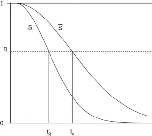
j = 1,2, . . . , N. For q ∈ (0,1), the inverse values of the lower and upper
survival functions of Tn+1 in (4) and (5), can be defined as tq =S−1(q) = inf t∈R{S(t)6q} tq =S −1 (q) = inf t∈R {S(t)6q}
tq tq
0 1
q
S S
Figure 1: Illustration lower and upper survival functions
where tq ≤tq obviously holds as is illustrated in Figure 1.
It is reasonable to claim that the proposed semi-parametric predictive method performs well if the two following inequalities hold,
p1 = 1 N N X j=1 1(tjf >tjq)≤q p2 = 1 N N X j=1 1(tjf >tjq)≥q
We will investigate the performance in this manner by considering q = 0.25,0.50,0.75. One could of course investigate different quantiles but these values will provide a reasonably general picture of the performance of the method, together with some particular aspects which are important to il-lustrate. If one was specifically interested in, e.g., the performance of this method for extreme values, one could consider the corresponding quantile(s) to evaluate the performance of our method, detailed investigation of the per-formance for a wider range of inferences is left as a topic for future research.
To perform the simulation, we consider different values of Kendall’s τ. For each value of τ we simulate from an assumed parametric copula with the parameter set equal to the value which corresponds to τ. We consider two main scenarios: first that, in our semi-parametric method, we actually assume a copula from the same parametric family as used for simulation, and secondly that the assumed parametric copula belongs to a different family. For the first case, we expect the method to perform well. Of course, this scenario is highly unlikely in practice, but it is important to study the per-formance of the method in this case, and the simulations will also reveal some interesting facts about the level of imprecision in the predictive inferences. The second scenario is of more importance, as it represents a more likely practical situation, namely where a parametric copula is assumed but this is actually not fully in line with the data generating mechanism. This can be considered as misspecification, and it is in such scenarios that we hope our method will provide sufficient robustness to still provide relatively good quality predictive inference.
Given the simulated data in a run, we estimate the parameter of the assumed parametric copula using the pseudo maximum likelihood method which is included in the R package VineCopula [30]. As mentioned before, alternative estimation methods can be used; of course these may lead to slightly different results, but the overall performance of the method is unlikely to be affected much by minor differences in the estimation method. With the estimate ˆθ for the copula parameter, we obtain the probabilities hij(ˆθ)
as given in Equation (1), and these form the basis for any possible inferences of interest.
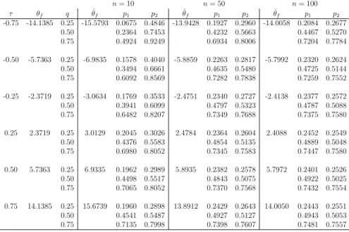
We have run N = 10,000 simulations with sample sizes n = 10,50,100, and with q = 0.25,0.50,0.75 and τ = −0.75,−0.5,−0.25,0,0.25,0.5,0.75. We restricted attention to the four parametric copulas discussed in Section 1, noting that the Frank copula does not allowτ = 0. Due to space limitations we only report a small subset of the simulations we ran; for each reported case we report the results of the first simulation we performed, later ones gave very similar results which led to identical conclusions.
First, we applied our semi-parametric method with the assumed copula actually belonging to the same parametric family used for the data genera-tion. Tables 1 and 2 present the results for the Normal and Frank copula, respectively (for the Clayton and Gumbel copulas results were very similar and led to the same conclusions). These tables report the values p1 and p2
For good performance of our method, we require p1 ≤q≤ p2. Furthermore,
these tables also present a value ˆθ, this is the average of the 10,000 estimates of the parameter, so for these two tables this value is expected to be close to the value for θ which corresponds directly to theτ used, and which is given in the second column of each table. However, we will not focus on these estimated values as it is really the predictive performance that is important to consider, due to the predictive nature of our approach. It is clear though that the parameter estimates tend to be closer to the real value for larger values of n, which is of course fully as expected. It may be of interest to implement other estimation methods for the copula parameter, which may provide a slightly better performance, detailed study of this is left as a topic for future research.
All cases in Tables 1 and 2 haveq ∈[p1, p2], which shows an overall good
performance of our semi-parametric predictive method, which is fully in line with expectations due to the use of the same parametric copula family in our method as the one that was actually used to simulate the data.
These tables illustrate two important aspects of the imprecision in our method. First, for corresponding cases with increasing n, the imprecision, reflected through the difference p2 −p1, decreases. This is logical from the
perspective that more data allow more precise inferences, which is common in statistical methods using imprecise probabilities [2]. Indeed, if one increases the value of n further, imprecision will decrease to 0 in the limit, where, informally, limit arguments are based on NPI for the marginals converging to the empirical marginal distributions, which in turn will converge to the underlying distributions, and with the assumed copula actually belonging to the same family as the one used to generate the data, this also will ensure an increasingly good performance of the method for increasing n.
A perhaps somewhat less expected feature of our method is seen by com-paring corresponding cases with the same absolute value of τ, but negative
τ compared to positive τ. For such cases, the imprecision p2−p1 is always
greater with the negative correlation than with the positive correlation, and this effect is stronger the larger the absolute value of the correlation. This feature occurs due to the fact that we are considering events that the sum
Tn+1 = Xn+1+Yn+1 exceeds values t, and can be explained by considering
the probabilitieshij(ˆθ) which are the key ingredients of our method for
infer-ence. In case of positive correlation, the hij(ˆθ) tend to be largest for values
for values of i and j with sum near to n+ 2, and this effect is stronger the larger the absolute value of the correlation. Calculating the lower and upper probabilities (4) and (5) tends to include several more hij(ˆθ) values in the
latter than in the former, and for events Tn+1 > tthese extrahij(ˆθ) included
in the upper probability tend to have the sum of their subscripts i and j
about constant. Hence, for positive correlation these extra hij(ˆθ) tend to
include a few larger values for most values of t. For negative correlation the effect is quite different, as then these extra hij(ˆθ) tend to include relatively
small values for small and for large values of t, in relation to the observed data, but when t is closer to the center of the empirical distribution of the values xi +yi, corresponding to the n data pairs (xi, yi), then many of the
extra hij(ˆθ) are quite large, resulting in large imprecision. This effect can
also be seen from plots of the lower and upper survival functions for Tn+1,
where positive correlation leads to imprecision being fairly similar over the whole range, while for negative correlation there is little imprecision in the tails but much imprecision near the center of the empirical distribution of the
xi+yi. As these lower and upper survival functions do not illustrate further
relevant aspects for the discussion, we have not included a figure here, but we do include such a figure in an example in Section 5, where we will emphasize this issue again.
As mentioned before, the main idea of the new method presented in this paper is to provide a quite straightforward method for prediction of a bivari-ate random quantity, where imprecision in the marginals provides robustness with regard to the assumed copula. This is attractive in practice, because one often has less knowledge about the dependence structure than about the marginals, in particular if one has a relatively small data set available. The practical usefulness of the method is therefore dependent on its ability to provide reasonable quality predictive inference in case one does not as-sume to know exactly the parametric family of copulas which generated the data. To study the performance of our semi-parametric predictive inference method, we perform simulations as before, but now we generate the data from one of the four mentioned copula families, while we assume a different parametric copula for the second step of our method. The simulations are further performed in the same manner as those above, with attention again on prediction of Tn+1 =Xn+1+Yn+1.
We report again first simulation results for just a few scenarios, the other combinations of real and assumed copulas, out of the four parametric
cop-n= 10 n= 50 n= 100 τ θn q θˆn p1 p2 θˆn p1 p2 θˆn p1 p2 -0.75 -0.9239 0.25 -0.9181 0.0854 0.5099 -0.9212 0.2002 0.3015 -0.9228 0.2202 0.2761 0.50 0.2477 0.7533 0.4187 0.5871 0.4566 0.5544 0.75 0.4911 0.9153 0.7045 0.8026 0.7311 0.7810 -0.50 -0.7071 0.25 -0.7462 0.1534 0.4002 -0.7235 0.2355 0.2919 -0.7169 0.2465 0.2691 0.50 0.3342 0.6466 0.4641 0.5529 0.4848 0.5292 0.75 0.5798 0.8355 0.7252 0.7797 0.7344 0.7604 -0.25 -0.3827 0.25 -0.4473 0.1942 0.3672 -0.4128 0.2406 0.2767 -0.3827 0.2477 0.2660 0.50 0.3943 0.6121 0.4728 0.5296 0.4863 0.5173 0.75 0.6386 0.8084 0.7303 0.7639 0.7370 0.7541 0.00 0 0.25 -0.0010 0.1877 0.3139 -0.0008 0.2362 0.2635 0.0000 0.2431 0.2566 0.50 0.4102 0.5723 0.4711 0.5105 0.4933 0.5141 0.75 0.6665 0.7971 0.7323 0.7626 0.7466 0.7598 0.25 0.3827 0.25 0.4478 0.1847 0.2956 0.4113 0.2279 0.2505 0.4004 0.2454 0.2556 0.50 0.4286 0.5538 0.4766 0.5074 0.4908 0.5026 0.75 0.6968 0.8057 0.7369 0.7580 0.7437 0.7540 0.50 0.7071 0.25 0.7469 0.2011 0.2931 0.7224 0.2394 0.2595 0.7164 0.2440 0.2525 0.50 0.4500 0.5554 0.4788 0.5033 0.4898 0.5026 0.75 0.7021 0.7978 0.7326 0.7537 0.7489 0.7602 0.75 0.9239 0.25 0.9174 0.2009 0.2865 0.9211 0.2430 0.2629 0.9224 0.2417 0.2524 0.50 0.4465 0.5441 0.4980 0.5168 0.4933 0.5039 0.75 0.6986 0.7961 0.7411 0.7607 0.7430 0.7527 Table 1: Predictive performance, Normal copula
n= 10 n= 50 n= 100 τ θf q θˆf p1 p2 θˆf p1 p2 θˆf p1 p2 -0.75 -14.1385 0.25 -15.5793 0.0675 0.4846 -13.9428 0.1927 0.2960 -14.0058 0.2084 0.2677 0.50 0.2364 0.7453 0.4232 0.5663 0.4467 0.5270 0.75 0.4924 0.9249 0.6934 0.8006 0.7204 0.7784 -0.50 -5.7363 0.25 -6.9835 0.1578 0.4040 -5.8859 0.2263 0.2817 -5.7992 0.2320 0.2624 0.50 0.3494 0.6661 0.4635 0.5480 0.4725 0.5144 0.75 0.6092 0.8569 0.7282 0.7838 0.7259 0.7552 -0.25 -2.3719 0.25 -3.0634 0.1769 0.3533 -2.4751 0.2340 0.2727 -2.4138 0.2377 0.2572 0.50 0.3941 0.6099 0.4797 0.5323 0.4787 0.5088 0.75 0.6482 0.8207 0.7349 0.7688 0.7375 0.7580 0.25 2.3719 0.25 3.0129 0.2045 0.3026 2.4784 0.2364 0.2604 2.4088 0.2452 0.2549 0.50 0.4376 0.5583 0.4854 0.5135 0.4889 0.5048 0.75 0.6980 0.8052 0.7345 0.7583 0.7447 0.7580 0.50 5.7363 0.25 6.9335 0.1962 0.2989 5.8935 0.2382 0.2578 5.7972 0.2401 0.2526 0.50 0.4498 0.5517 0.4843 0.5075 0.4922 0.5025 0.75 0.7065 0.8052 0.7370 0.7568 0.7432 0.7554 0.75 14.1385 0.25 15.6739 0.1960 0.2898 13.8912 0.2429 0.2643 14.0050 0.2443 0.2551 0.50 0.4541 0.5487 0.4927 0.5127 0.4943 0.5053 0.75 0.7135 0.7998 0.7398 0.7607 0.7481 0.7557
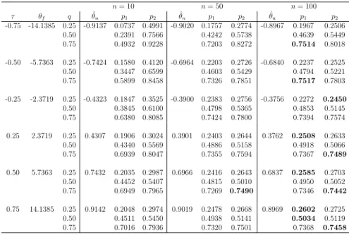
ula families discussed before, provided very similar results, as did repeated simulations of the same scenarios. Table 3 presents the results with data generated from the Frank copula whilst assuming the Normal copula in our method. While we mostly focus on the predictive performance, it is impor-tant to briefly consider the parameter estimate ˆθn. Of course, this is not an
estimate of the parameter θf as used in the Frank copula for generating the
data, the values θn corresponding to the respective values for τ are given in
Table 1. These estimated values for θn are now a bit further from the values
given in Table 1, which results from the fact that the data are not generated from the Normal copula but from the Frank copula.
It is more important to consider the predictive performance of our method. The values of p1 and p2 in Table 3 are mostly pretty similar to those in
Ta-bles 1 and 2, although there are now a few cases for which q is not contained in the interval [p1, p2]. These are high-lighted by bold font numbers in the
table. For n = 10 there are no such cases, indeed the imprecision in the method provides sufficient robustness to still have q ∈ [p1, p2]. For n = 50
this is also mostly the case, although there is one case here, for τ = 0.5 and
q = 0.75, where p2 < q, albeit only just. For n= 100 there are substantially
more cases where the interval [p1, p2] does not contain the corresponding q,
although in these cases q tends to be only just outside the interval. This is in line with expectation, because for larger n the method has only small imprecision on the marginals, hence these provide less robustness against the misspecification of the dependence structure, so assuming the wrong para-metric copula starts to have a stronger effect. Table 4 presents the results of a similar simulation with the data generated from the Normal copula and the Frank copula assumed in our method. The results for this case are very similar to those just described.
For larger numbers of data, such as n = 100 or more, one could add methods for model selection to our method, to try to find a parametric copula that fits well with the data. While this will be of interest, we intend to focus future research in a different direction, namely by applying nonparametric copula methods combined with NPI for the marginals for larger data sets, in order to arrive at predictive inference which is fully flexible to adapt to the data.
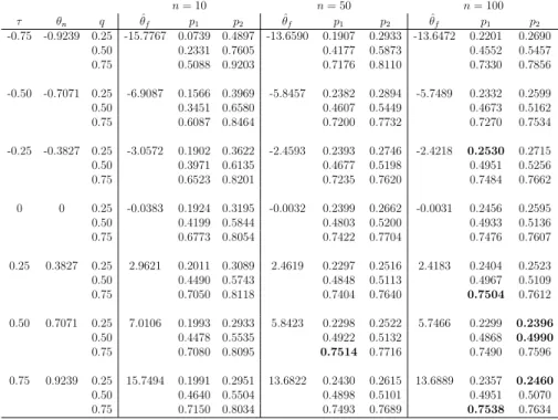
Tables 5 and 6 present the results of similar simulation studies with data generated from the Clayton and Gumbel copulas, respectively. For both these cases the Frank copula was assumed for our method; in further simulations with the Normal copula assumed instead the results were very similar. For
n= 10 n= 50 n= 100 τ θf q θˆn p1 p2 θˆn p1 p2 θˆn p1 p2 -0.75 -14.1385 0.25 -0.9137 0.0737 0.4991 -0.9020 0.1757 0.2774 -0.8967 0.1967 0.2506 0.50 0.2391 0.7566 0.4242 0.5738 0.4639 0.5449 0.75 0.4932 0.9228 0.7203 0.8272 0.7514 0.8018 -0.50 -5.7363 0.25 -0.7424 0.1580 0.4120 -0.6964 0.2203 0.2726 -0.6840 0.2237 0.2525 0.50 0.3447 0.6599 0.4603 0.5429 0.4794 0.5221 0.75 0.5899 0.8458 0.7326 0.7851 0.7517 0.7803 -0.25 -2.3719 0.25 -0.4323 0.1847 0.3525 -0.3900 0.2383 0.2756 -0.3756 0.2272 0.2450 0.50 0.3845 0.6100 0.4798 0.5365 0.4853 0.5145 0.75 0.6380 0.8085 0.7424 0.7800 0.7394 0.7574 0.25 2.3719 0.25 0.4307 0.1906 0.3024 0.3901 0.2403 0.2644 0.3762 0.2508 0.2633 0.50 0.4340 0.5569 0.4886 0.5158 0.4918 0.5066 0.75 0.6939 0.8047 0.7355 0.7594 0.7367 0.7489 0.50 5.7363 0.25 0.7432 0.2035 0.2987 0.6966 0.2416 0.2643 0.6837 0.2585 0.2703 0.50 0.4452 0.5407 0.4815 0.5010 0.4950 0.5052 0.75 0.6949 0.7965 0.7269 0.7490 0.7346 0.7442 0.75 14.1385 0.25 0.9142 0.2048 0.2974 0.9019 0.2478 0.2668 0.8969 0.2602 0.2725 0.50 0.4511 0.5450 0.4938 0.5141 0.5034 0.5119 0.75 0.7016 0.7936 0.7320 0.7501 0.7368 0.7458
Table 3: Simulations from Frank copula; Normal copula assumed for inference
n = 10 the robustness is again sufficient to always get q ∈ [p1, p2], indeed
we have not encountered any simulation, for any combination of these four copulas, where this was not the case. For n = 50 and n = 100 the results are now slightly worse than before, but whereq is outside the interval [p1, p2]
it is always close to it. This reflects that the Clayton and Gumbel copulas differ more from the Frank copula than the Normal copula does. We also included the case n= 30 here, for which the results were all fine.
This simulation study has illustrated our new semi-parametric method and revealed some interesting aspects, as discussed above. The main conclu-sion we draw from it, is that for small values of n the imprecision provides sufficient robustness for the predictive inferences to have good frequentist properties. This depends on the copulas used, the random quantity con-sidered, and also the percentiles considered. Differences would show more strongly if one considers quite extreme percentiles. If data were generated with a very different dependence structure than can be modelled through the assumed parametric copula, then the method would also perform worse. However, we would hope that in such cases, either there is background knowl-edge about the dependence structure, which can be used to select a more suitable copula, or that the data already show a certain pattern to make us aware of the unlikely success of the proposed method with a basic
cop-n= 10 n= 50 n= 100 τ θn q θˆf p1 p2 θˆf p1 p2 θˆf p1 p2 -0.75 -0.9239 0.25 -15.7767 0.0739 0.4897 -13.6590 0.1907 0.2933 -13.6472 0.2201 0.2690 0.50 0.2331 0.7605 0.4177 0.5873 0.4552 0.5457 0.75 0.5088 0.9203 0.7176 0.8110 0.7330 0.7856 -0.50 -0.7071 0.25 -6.9087 0.1566 0.3969 -5.8457 0.2382 0.2894 -5.7489 0.2332 0.2599 0.50 0.3451 0.6580 0.4607 0.5449 0.4673 0.5162 0.75 0.6087 0.8464 0.7200 0.7732 0.7270 0.7534 -0.25 -0.3827 0.25 -3.0572 0.1902 0.3622 -2.4593 0.2393 0.2746 -2.4218 0.2530 0.2715 0.50 0.3971 0.6135 0.4677 0.5198 0.4951 0.5256 0.75 0.6523 0.8201 0.7235 0.7620 0.7484 0.7662 0 0 0.25 -0.0383 0.1924 0.3195 -0.0032 0.2399 0.2662 -0.0031 0.2456 0.2595 0.50 0.4199 0.5844 0.4803 0.5200 0.4933 0.5136 0.75 0.6773 0.8054 0.7422 0.7704 0.7476 0.7607 0.25 0.3827 0.25 2.9621 0.2011 0.3089 2.4619 0.2297 0.2516 2.4183 0.2404 0.2523 0.50 0.4490 0.5743 0.4848 0.5113 0.4967 0.5109 0.75 0.7050 0.8118 0.7404 0.7640 0.7504 0.7612 0.50 0.7071 0.25 7.0106 0.1993 0.2933 5.8423 0.2298 0.2522 5.7466 0.2299 0.2396 0.50 0.4478 0.5535 0.4922 0.5132 0.4868 0.4990 0.75 0.7080 0.8095 0.7514 0.7716 0.7490 0.7596 0.75 0.9239 0.25 15.7494 0.1991 0.2951 13.6822 0.2430 0.2615 13.6889 0.2357 0.2460 0.50 0.4640 0.5504 0.4898 0.5101 0.4951 0.5070 0.75 0.7150 0.8034 0.7493 0.7689 0.7538 0.7634
Table 4: Simulations from Normal copula; Frank copula assumed for inference
n= 10 n= 30 n= 50 n= 100 τ θc q ˆθf p1 p2 θˆf p1 p2 θˆf p1 p2 θˆf p1 p2 0.25 0.6667 0.25 3.0639 0.1809 0.2959 2.5553 0.2214 0.2637 2.5017 0.2313 0.2567 2.4415 0.2375 0.2493 0.50 0.4424 0.5745 0.4970 0.5457 0.5058 0.5338 0.5181 0.5329 0.75 0.7001 0.7985 0.7401 0.7762 0.7498 0.7733 0.7545 0.7645 0.50 2.0000 0.25 7.1205 0.1866 0.2968 6.0366 0.2177 0.2572 5.8780 0.2254 0.2505 5.7896 0.2284 0.2416 0.50 0.4630 0.5732 0.4958 0.5354 0.5081 0.5321 0.5144 0.5259 0.75 0.7095 0.7975 0.7305 0.7612 0.7433 0.7618 0.7534 0.7636 0.75 6.0000 0.25 16.3807 0.1904 0.2908 13.9919 0.2298 0.2642 13.8441 0.2355 0.2580 13.7415 0.2458 0.2575 0.50 0.4670 0.5626 0.4915 0.5248 0.4962 0.5149 0.5031 0.5134 0.75 0.7107 0.7953 0.7387 0.7686 0.7412 0.7583 0.7531 0.7619
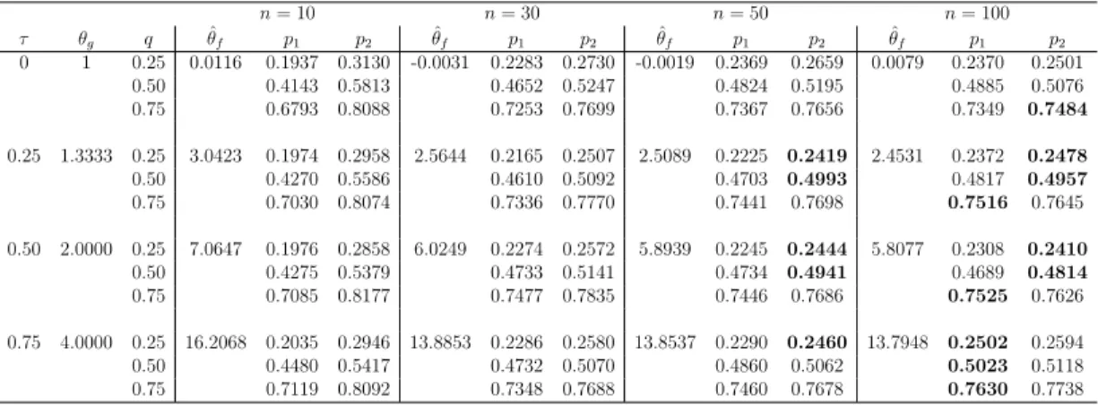
n= 10 n= 30 n= 50 n= 100 τ θg q ˆθf p1 p2 θˆf p1 p2 θˆf p1 p2 θˆf p1 p2 0 1 0.25 0.0116 0.1937 0.3130 -0.0031 0.2283 0.2730 -0.0019 0.2369 0.2659 0.0079 0.2370 0.2501 0.50 0.4143 0.5813 0.4652 0.5247 0.4824 0.5195 0.4885 0.5076 0.75 0.6793 0.8088 0.7253 0.7699 0.7367 0.7656 0.7349 0.7484 0.25 1.3333 0.25 3.0423 0.1974 0.2958 2.5644 0.2165 0.2507 2.5089 0.2225 0.2419 2.4531 0.2372 0.2478 0.50 0.4270 0.5586 0.4610 0.5092 0.4703 0.4993 0.4817 0.4957 0.75 0.7030 0.8074 0.7336 0.7770 0.7441 0.7698 0.7516 0.7645 0.50 2.0000 0.25 7.0647 0.1976 0.2858 6.0249 0.2274 0.2572 5.8939 0.2245 0.2444 5.8077 0.2308 0.2410 0.50 0.4275 0.5379 0.4733 0.5141 0.4734 0.4941 0.4689 0.4814 0.75 0.7085 0.8177 0.7477 0.7835 0.7446 0.7686 0.7525 0.7626 0.75 4.0000 0.25 16.2068 0.2035 0.2946 13.8853 0.2286 0.2580 13.8537 0.2290 0.2460 13.7948 0.2502 0.2594 0.50 0.4480 0.5417 0.4732 0.5070 0.4860 0.5062 0.5023 0.5118 0.75 0.7119 0.8092 0.7348 0.7688 0.7460 0.7678 0.7630 0.7738
Table 6: Simulations from Gumbel copula; Frank copula assumed for inference
ula. Overall, this work fits in a larger project where the idea is that, for larger sample sizes, the parametric copula in our method can be replaced by a nonparametric copula. We expect that this would be of benefit for larger sample sizes. Hence, the idea is that a combination of the use of a convenient parametric copula for smaller sample sizes, and a nonparametric copula for larger sample sizes, provides a suitable predictive inference method for bivari-ate data. This raises substantial questions, which are considered in ongoing research.
5. Examples
In this section, two examples are presented to illustrate application of the proposed semi-parametric predictive method. The data sets are quite small, for which the study in Section 4 showed that our method provides good robustness with regard to choice of copula due to quite substantial imprecision resulting mostly from the use of NPI for the marginals. We only present results using one family of parametric copulas in each example. When we applied the other parametric copulas used in this paper we got results that were very close to those reported here. More details of these further investigations, and also of additional simulation studies, are reported in the PhD thesis of the third-named author [26].
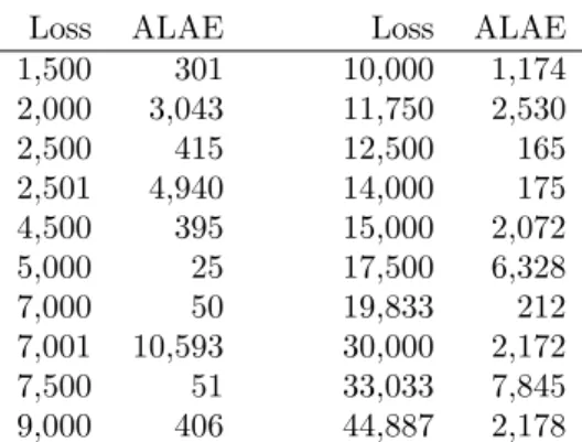
Example 5.1. Consider the data set in Table 7 on casuality insurance [23, p. 403], which record both the loss and the expenses that are directly related to
Loss ALAE Loss ALAE 1,500 301 10,000 1,174 2,000 3,043 11,750 2,530 2,500 415 12,500 165 2,501 4,940 14,000 175 4,500 395 15,000 2,072 5,000 25 17,500 6,328 7,000 50 19,833 212 7,001 10,593 30,000 2,172 7,500 51 33,033 7,845 9,000 406 44,887 2,178
Table 7: Losses and corresponding ALAE values, Example 5.1
the payment of the loss (the ‘allocated loss adjustment expenses’, ALAE) for an insurance company on twenty claims. The loss and the ALAE are usually positively correlated [23], there is some suggestion that this is also the case in these data as can be seen from Figure 2. The original data consist of 24 bivariate data observations, to illustrate our approach we have removed four ‘outliers’ and we have adjusted the data to avoid tied observations (namely 2501, 7001, 51 are used instead of 2500, 7000, 50). There is no strong need to exclude outlying data from the analysis when our semi-parametric method is used, but the effect of data which influence the copula estimation very strongly requires further study, for example into the use of copulas with multiple parameters that can separate different dependence relations over the ranges of the data considered. This is left as an important topic for future research, in particular to compare when it is better to use more complicated parametric copulas and when it is better to use nonparametric copulas.
In line with the earlier presentation in this paper, Loss will be the X
variable and ALEA the Y variable. Suppose that we are interested in the event that the sum of the next Loss and ALAE will exceed t, that is
Tn+1 =Xn+1+Yn+1 > t, based on the available data (xi, yi),i= 1,2, . . . ,20.
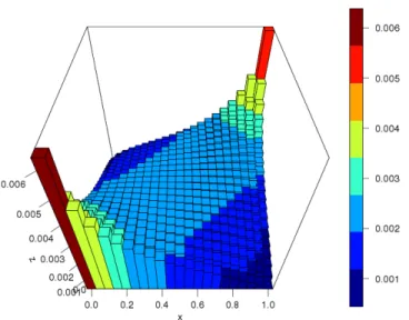
We apply the new semi-parametric method presented in Section 3, where we assume a Normal copula and again use pseudo maximum likelihood estima-tion as available in the R package VineCopula [30]. The probabilities hij(ˆθ)
in our method, resulting from the parameter estimation with the Normal cop-ula, are presented in Figure 3, which clearly shows the positive correlation betweenXen+1 andYen+1, and hence betweenXn+1 and Yn+1, in this example.
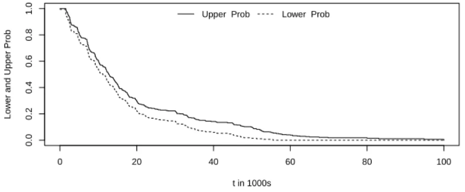
The lower and upper probabilities for the eventTn+1 > tare presented in
● ● ● ● ● ● ● ● ● ● ● ● ● ● ● ● ● ● ● ● 0 10 20 30 40 0 20 40 60 80 100 Loss in 1000s ALAE in 100s
Figure 2: Losses and corresponding ALAE values, Example 5.1
0 20 40 60 80 100 0.0 0.2 0.4 0.6 0.8 1.0 t in 1000s Lo w
er and Upper Prob
Upper Prob Lower Prob
Figure 4: Lower and upper probabilities forTn+1> t, Example 5.1
in a variety of ways, depending on the actual question of interest. Figure 4 shows that the imprecision, reflected through the difference between corre-sponding upper and lower probabilities, is pretty similar through the main range of empirical values for xi +yi. This is due to the effect discussed for
the simulations in Section 4, namely the positive correlation between Loss and ALEA combined with interest in the sum of these quantities. If the data would have indicated a negative correlation, then imprecision would vary more substantially when interested in the sum of the two quantities; simi-larly, with positive correlation in the data, imprecision would also vary more substantially if one is interested in the difference of the two random quanti-ties. Such effects on our method can be studied in detail by considering the probabilities hij(ˆθ). tin 1000s P(Tn+1> t) P(Tn+1> t) tin 1000s P(Tn+1> t) P(Tn+1> t) 0 0.9936 1.0000 45 0.0446 0.1290 5 0.7619 0.8145 50 0.0150 0.0994 10 0.5452 0.6071 55 0.0064 0.0582 15 0.3571 0.4257 60 0.0000 0.0386 20 0.2264 0.2990 65 0.0000 0.0245 25 0.1617 0.2366 70 0.0000 0.0185 30 0.1455 0.2226 75 0.0000 0.0185 35 0.0869 0.1664 80 0.0000 0.0150 40 0.0600 0.1418 85 0.0000 0.0110
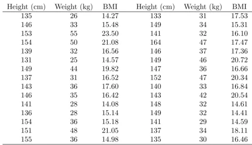
Height (cm) Weight (kg) BMI Height (cm) Weight (kg) BMI 135 26 14.27 133 31 17.53 146 33 15.48 149 34 15.31 153 55 23.50 141 32 16.10 154 50 21.08 164 47 17.47 139 32 16.56 146 37 17.36 131 25 14.57 149 46 20.72 149 44 19.82 147 36 16.66 137 31 16.52 152 47 20.34 143 36 17.60 140 33 16.84 146 35 16.42 143 42 20.54 141 28 14.08 148 32 14.61 136 28 15.14 149 32 14.41 154 36 15.18 141 29 14.59 151 48 21.05 137 34 18.11 155 36 14.98 135 30 16.46
Table 9: The heights (cm), weights (kg) and BMI of 30 eleven-year-old girls, Example 5.2
Example 5.2. Thus far, we have illustrated our method by considering the sum of the two values in the next bivariate observation, Xn+1 +Yn+1. In
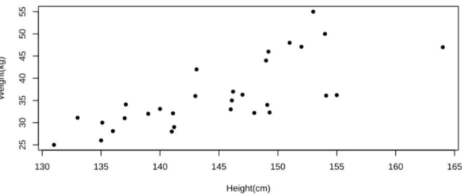
order to illustrate application to scenarios where interest is in a different function of (Xn+1, Yn+1), consider the data presented in Table 9 and Figure
5 [18]. These present the heights (cm) and weights (kg) of n = 30 eleven-year-old girls attending Heaton Middle School in Bradford. Suppose that one is interested in the body-mass index (BMI) of a further girl, where one can imagine there having been 31 girls with one selected randomly to not be included in the data set, and whose BMI one would wish to predict after learning the heights and weights of the other 30 girls. Interest in the BMI may be in order to investigate whether they have healthy weight, are underweight or overweight, or even obese, so we derive the lower and upper probabilities for the thirty-first girl to be in each of these categories, based on our semi-parametric method. The BMI is calculated using the well-known formula,
BMI = Weight (kg) [Height (m)]2
For this illustrative example, we use the classification of BMI values pro-vided by the Center for Disease Control and Prevention (www.cdc.gov), ac-cording to which an eleven-year-old girl is considered underweight if her BMI is less than 14.08, has healthy weight if the BMI is between 14.08 and 19.50, is overweight if the BMI is between 19.50 and 24.14, and obese if the BMI is
● ● ● ● ● ● ● ● ● ● ● ● ● ● ● ● ● ● ● ● ● ● ● ● ● ● ● ● ● ● 130 135 140 145 150 155 160 165 25 30 35 40 45 50 55 Height(cm) W eight(kg)
Figure 5: The heights (cm) and weights (kg) of 30 eleven-year-old girls, Example 5.2
BMI∈ P P
Underweight [6.92,14.08) 0.0303 0.1010
Healthy weight [14.08,19.50) 0.6521 0.8107
Overweight [19.50, 24.14) 0.1368 0.2456
Obese [24.14, 38.40) 0.0013 0.0222
Table 10: NPI lower and upper probabilities, Example 5.2
at least 24.14. The lower and upper probabilities for these events of interest, calculated using Equations (2) and (3) and using again the Normal copula with the same estimation method as before, are given in Table 10. To avoid difficulties due to the functional form of the BMI, we restricted the range of ‘possible’ values for the height and weight quantities by setting finite end-points for the ranges used in NPI for the marginals. We set these values at
x0 = 125, x31 = 170, y0 = 20 and y31 = 60, which seem quite realistic and
lead to corresponding minimum BMI 6.92 and maximum BMI 38.40, which are included in the ranges in Table 10. Choosing different values for x0, x31, y0 and y31 will have some impact on the lower and upper probabilities
re-sulting from our method, but the effect of minor differences to these values is neglectable.
6. Concluding remarks
This paper presents a new semi-parametric method for predictive infer-ence about a future bivariate observation, which can be used to consider any
function of interest involving the two quantities in such an observation. It combines NPI on the marginals, which is predictive by nature, with the use of a parametric copula to take dependence into account, where the parame-ter of the copula is estimated based on available data. This method can be used with a wide variety of estimation methods because only a single point estimator is used. A possible generalization of the method is by introduc-ing some further robustness, or imprecision, in the copula, either by usintroduc-ing a range of parameter values (e.g. related to a confidence interval) or a set of copulas. Implementing these straightforward ideas would require further research, as they would lead to imprecise probabilities instead of the precise probabilities hij(ˆθ) which are central to our method.
By combining NPI with an estimated copula, the proposed method does not fully adopt the strong frequentist properties of NPI, and hence has a heuristic nature. We have investigated its performance via simulation studies, more detailed research of its performance in a wider range of applications will be of benefit. The main thesis of this research, going beyond this paper, is that the robustness provided by our method, with the use of a quite basic copula, will often lead to satisfactory inferences for small to medium sized data sets. For large data sets, it is expected that the method can be applied with a nonparametric copula, this is the topic of ongoing research.
Throughout this work, we restricted attention to a single future obser-vation. In practice, one may be interested in multiple future observations, in NPI the inter-dependence of such multiple future observations is taken into account [7]. It will be of interest to develop this bivariate method for multiple future observations. NPI has recently been presented for a num-ber of inferential problems, including accuracy of diagnostic tests [10, 11], inferences with right-censored observations [9] and reproducibility of basic nonparametric tests [8]. For all such applications, it is of interest to develop predictive methodology for bivariate, and more generally multivariate data. The approach presented in this paper may be a suitable starting point for research on these topics.
A major advantage of the presented method is its relatively easy com-putations, as the use of NPI on the marginals combines naturally with the discretization of the copula. Hence, the computational complexity is only with regard to the estimation of the copula parameter, which for the copulas considered in this paper is a routine procedure for which standard software is available. It may be attractive to use copulas with multi-dimensional pa-rameters, which would provide better opportunities to take more information
about dependence in the data into account. As long as suitable estimation methods are available, this can be implemented in our method without any difficulties.
The bivariate method presented here can straightforwardly be general-ized to multivariate data, where the curse of dimensionality implies that the number of data required to get meaningful inferences grows exponentially with the dimension of the data. We restricted attention to the bivariate case in order to illustrate and investigate the method, application to higher dimensional situations is an important topic for future research.
Finally, it is important to emphasize that the method presented in this paper has a novel aspect within statistical theory using imprecise probabili-ties. Traditionally, imprecision is used particularly on aspects for which one has relatively little information. Here, however, we use imprecision on the marginals but not on the copula, while the data tend to contain less informa-tion about the dependence structure than about the marginals. This is done as the imprecision on the marginals provides robustness with regard to the copula choice, with the added benefit that the imprecise probability method used on the marginals is easy to implement and fits naturally to discretiza-tion of the copula. This idea, to add imprecision to the easier part of an inference in order to provide robustness for the harder part, and all together simplifying computation, promises to have wider applicability, for example in big data scenarios where fast computation is crucial. We will explore this idea in other settings in future research.
Acknowledgements
We are grateful to an anonymous reviewer for supportive comments and suggestions to improve the presentation of this paper.
References
[1] Augustin T., Coolen F.P.A. (2004). Nonparametric predictive inference and interval probability. Journal of Statistical Planning and Inference
[2] Augustin T., Coolen F.P.A., de Cooman G., Troffaes, M.C.M. (Eds.) (2014). Introduction to Imprecise Probabilities. Wiley, Chichester. [3] Chen X., Fan Y., Tsyrennikov V. (2006). Efficient estimation of
semi-parametric multivariate copula models.Journal of the American Statis-tical Association 101, 1228-1240.
[4] Cherubini U., Luciano E., Vecchiato W. (2004). Copula Methods in Fi-nance. Wiley, Chichester.
[5] Clayton D.G. (1978). A model for association in bivariate life tables and its application in epidemiological studies of familial tendency in chronic disease incidence. Biometrika 65 141-151.
[6] Coolen F.P.A. (2006). On nonparametric predictive inference and objec-tive Bayesianism.Journal of Logic, Language and Information1521-47. [7] Coolen F.P.A. (2011). Nonparametric predictive inference. In: Lovric M. (Ed.),International Encyclopedia of Statistical Science. Springer, Berlin, pp. 968-970.
[8] Coolen F.P.A., Bin Himd S. (2014). Nonparametric predictive inference for reproducibility of basic nonparametric tests. Journal of Statistical Theory and Practice 8 591-618.
[9] Coolen-Maturi T., Coolen F.P.A. (2015). Nonparametric predictive in-ference with combined data under different right-censoring schemes. Journal of Statistical Theory and Practice 9 288-304.
[10] Coolen-Maturi T., Coolen-Schrijner P., Coolen, F.P.A. (2012). Nonpara-metric predictive inference for binary diagnostic tests. Journal of Sta-tistical Theory and Practice 6665-680.
[11] Elkhafifi F.F., Coolen F.P.A. (2012). Nonparametric predictive inference for accuracy of ordinal diagnostic tests.Journal of Statistical Theory and Practice 6 681-697.
[12] De Finetti B. (1974). Theory of Probability. Wiley, Chichester.
[13] Embrechts P., Lindskog F., McNeil A. (2003). Modelling dependence with copulas and applications to risk management. In: Rachev S.T.
(Ed.), Handbook of Heavy Tailed Distributions in Finance (Vol. 1). North-Holland, Amsterdam, pp. 329-384.
[14] Frank M.J. (1979). On the simultaneous associativity of f(x, y) and
x+y−f(x, y).Aequationes Mathematicae 19 194-226.
[15] Frees E.W., Valdez E.A. (1998). Understanding relationships using cop-ulas. North American Actuarial Journal 2 1-25.
[16] Genest C., Favre A. (2007). Everything you always wanted to know about copula modeling but were afraid to ask. Journal of Hydrologic Engineering 12 347-368.
[17] Gumbel E.J. (1960). Distributions des valeurs extremes en plusieurs di-mensions. Publications de l’Institute de Statist´ıque de l’Universit´e de Paris 9 171-173.
[18] Hand D.J., Daly F., Lunn A.D., McConway K.J., Ostrowski E. (1994). A Handbook of Small Data Sets. Chapman & Hall, London.
[19] Hill B.M. (1968). Posterior distribution of percentiles: Bayes’ theorem for sampling from a population. Journal of the American Statistical As-sociation 63 677-691.
[20] Ignatieva K., Platen E., Rendek R. (2011). Using dynamic copulae for modeling dependency in currency denominations of a diversified world stock index. Journal of Statistical Theory and Practice 5 425-452. [21] Joe H. (1997). Multivariate Models and Multivariate Dependence
Con-cepts. Chapman & Hall, London.
[22] Joe H. (2005). Asymptotic efficiency of the two-stage estimation method for copula-based models. Journal of Multivariate Analysis 94 401-419. [23] Klugman S.A., Panjer H.H., Willmot G.E. (2012). Loss Models: From
Data to Decisions (4th Ed.). Wiley, New Jersey.
[24] Lawless J.F., Fredette M. (2005). Frequentist prediction intervals and predictive distributions. Biometrika92 529-542.
[25] Li J., Liu R.Y. (2008). Multivariate spacings based on data depth: I. Construction of nonparametric multivariate tolerance regions The An-nals of Statistics 36 1299-1323.
[26] Muhammad N. (2016). Predictive Inference with Copulas for Bivari-ate Data. PhD Thesis, Durham University, available from www.npi-statistics.com.
[27] Nelsen R.B. (2007). An Introduction to Copulas. Springer, New York. [28] Purcaru O. (2003). Semi-parametric archimedean copula modelling in
actuarial science. Insurance, Mathematics and Economics 33 419-420. [29] Rank J. (2007). Copulas: From Theory to Application in Finance. Risk
Books, London.
[30] Schepsmeier U., Stoeber J., Brechmann E.C. (2013). VineCop-ula: Statistical inference of vine copulas. R package version 1.1-1. http://CRAN.R-project.org/package=VineCopula
[31] Schick A., Wefelmeyer W. (2008). Some developments in semiparametric statistics. Journal of Statistical Theory and Practice 2 475-491.
[32] Sen S., Diawara N., Iftekharuddin K.M. Statistical pattern recognition using Gaussian copula. Journal of Statistical Theory and Practice, to appear.
[33] Sklar A.W. (1959). Fonctions de r´epartition `a n-dimension et leurs marges.Publications de l’Institut de Statistique de l’Universit´e de Paris
8 229-231.
[34] Tang X.S., Li D.Q., Zhou C.B., Zhang L.M. (2013). Bivariate distribu-tion models using copulas for reliability analysis. Journal of Risk and Reliability 227 499-512.
[35] Trivedi P.K., Zimmer D.M. (2005). Copula modeling: An introduction for practitioners. Foundations and Trends in Econometrics1 1-111. [36] Tsukahara H. (2005). Semiparametric estimation in copula models. The