A generalized LSTM-like training algorithm for
second-order recurrent neural networks
Derek D. Monner⇤, James A. Reggia
Department of Computer Science, University of Maryland, College Park, MD 20742, USA
Abstract
The Long Short Term Memory (LSTM) is a second-order recurrent neural net-work architecture that excels at storing sequential short-term memories and re-trieving them many time-steps later. To this point, the usefulness of the LSTM training algorithm has been limited by the fact that it can only be applied to a small set of network architectures. Here we introduce the Generalized Long Short-Term Memory (LSTM-g), which provides a local, efficient, LSTM-like training algorithm that can be applied without modification to a much wider range of second-order network architectures. With LSTM-g, all units have an identical set of operating instructions for both activation and learning, sub-ject only to the configuration of their local environment in the network; this is in contrast to LSTM, where each type of unit has its own activation and training instructions. When applied to LSTM-compatible architectures with peephole connections, LSTM-g takes advantage of an additional source of back-propagated error which can enable better performance than traditional LSTM. Enabled by the broad architectural applicability of LSTM-g, we demonstrate that training recurrent networks engineered for specific tasks can produce bet-ter results. We conclude that LSTM-g has the potential to both improve the performance and broaden the applicability of the LSTM family of gradient-based training algorithms for recurrent neural networks.
Keywords: recurrent neural network, gradient-based training, long short term
memory (LSTM), temporal sequence processing, sequential retrieval
1. Introduction
The Long Short Term Memory (LSTM) (Hochreiter & Schmidhuber, 1997) is a recurrent neural network architecture that combines fast training with ef-ficient learning on tasks that require sequential short-term memory storage for many time-steps during a trial. Since its inception, LSTM has been augmented
⇤Corresponding author. Telephone: +1 (301) 586-2495. Fax: (301) 405-6707.
Email addresses: [email protected](Derek D. Monner),[email protected](James A. Reggia)
and improved with forget gates (Gers & Cummins, 2000) and peephole connec-tions (Gers & Schmidhuber, 2000); despite this, LSTM’s usefulness is limited by the fact that it can only train a small set of second-order recurrent network architectures. By second-order neural network we mean one that not only al-lows normal weighted connections which propagate activation from one sending unit to one receiving unit, but also allows second-order connections: weighted connections fromtwo sending units to one receiving unit, where the signal re-ceived is dependent upon the product of the activities of the sending units with each other and the connection weight (Miller & Giles, 1993). When LSTM is described in terms of connection gating, as we discuss below, we see that the gate units serve as the additional sending units for the second-order connections. LSTM networks have an input layer, a hidden layer consisting of memory
block cell assemblies, and an output layer. Each memory block is composed
ofmemory cell units that retain state across time-steps, as well as three types of specialized gate units that learn to protect, utilize, or destroy this state as appropriate. The LSTM training algorithm back-propagates errors from the output units through the memory blocks, adjusting incoming connections of all units in the blocks, but then truncates the back-propagated errors. As a consequence, the LSTM algorithm cannot be used to e↵ectively train second-order networks with units placed between the memory blocks and the input layer. More generally, LSTM cannot be used to train arbitrary second-order recurrent neural architectures, as the error propagation and weight updates it prescribes are dependent upon the specific network architecture described in the original paper.
Motivated by a desire to explore alternate architectures more suited to spe-cific computational problems, we developed an algorithm we call Generalized Long Short-Term Memory (LSTM-g), an LSTM-like training algorithm that can be applied, without modification, to a much wider range of second-order recurrent neural networks. Each unit in an LSTM-g network has the same set of operating instructions, relying only on its local network environment to deter-mine whether it will fulfill the role of memory cell, gate unit, both, or neither. In addition, every LSTM-g unit is trained in the same way—a sharp contrast from LSTM, where each of several di↵erent types of units has a unique training regimen. LSTM-g reinterprets the gating of unit activations seen in LSTM; instead of gate units modulating other unit activations directly, they modulate the weights on connections between units. This change removes LSTM’s re-striction that memory cell states not be visible outside the corresponding block, allowing network designers to explore arbitrary architectures where gates can temporarily isolate one part of the network from another.
In addition to the expanded architectural applicability that it a↵ords, LSTM-g provides all of the benefits of the LSTM training algorithm when ap-plied to the right type of architecture. LSTM-g was designed to perform exactly the same weight updates as LSTM when applied to identical network architec-tures. However, on LSTM architectures with peephole connections, LSTM-g often performs better than the original algorithm by utilizing a source of back-propagated error that appears to have heretofore gone unnoticed.
In what follows, we present LSTM as previously described, followed by the generalized version. We then present an analysis of the additional error sig-nals which LSTM-g uses to its advantage, followed by experimental evidence that LSTM-g often performs better than LSTM when using the original tecture. Further experiments show that LSTM-g performs well on two archi-tectures specifically adapted to two computational problems. The appendices give the mathematical derivation of the LSTM-g learning rules and prove that LSTM-g is a generalization of LSTM.
2. LSTM
LSTM was developed as a neural network architecture for processing long temporal sequences of data. Other recurrent neural networks trained with vari-ants of back-propagation (Williams & Zipser, 1989; Werbos, 1990; Elman, 1990) proved to be ine↵ective when the input sequences were too long (Hochreiter & Schmidhuber, 1997). Analysis (summarized by Hochreiter & Schmidhuber (1997)) showed that for neural networks trained with back-propagation or other gradient-based methods, the error signal is likely to vanish or diverge as error travels backward through network space or through time. This is because, with every pass backwards through a unit, the error signal is scaled by the deriva-tive of the unit’s activation function times the weight that the forward signal traveled along. The further error travels back in space or time, the more times this scaling factor is multiplied into the error term. If the factor is consistently less than 1, the error will vanish, leading to small, ine↵ective weight updates; if it is greater than 1, the error term will diverge, potentially leading to weight oscillations or other types of instability. One way to preserve the value of the error is requiring the scaling factor to be equal to 1, which can only be con-sistently enforced with a linear activation function (whose derivative is 1) and a fixed weight ofwjj = 1. LSTM adopts this requirement for itsmemory cell
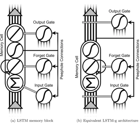
units, which have linear activation functions and self-connections with a fixed weight of 1 (Fig. 1a). This allows them to maintain unscaled activations and error derivatives across arbitrary time lags if they are not otherwise disturbed. Since back-propagation networks require nonlinear hidden unit activation func-tions to be e↵ective, each memory cell’s state is passed through a squashing function—such as the standard logistic function—before being passed on to the rest of the network.
The processing of long temporal sequences is complicated by the issue of interference. If a memory cell is currently storing information that is not use-ful now but will be invaluable later, this currently irrelevant information may interfere with other processing in the interim. This in turn may cause the infor-mation to be discarded, improving performance in the near term but harming it in the long term. Similarly, a memory cell may be perturbed by an irrelevant input, and the information that would have been useful later in the sequence can be lost or obscured. To help mitigate these issues, each memory cell has its net input modulated by the activity of another unit, termed aninput gate, and has its output modulated by a unit called anoutput gate (Fig. 1a). Each input
gate and output gate unit modulates one or a small number of memory cells; the collection of memory cells together with the gates that modulate them is termed amemory block. The gates provide a context-sensitive way to update the contents of a memory cell and protect those contents from interference, as well as protecting downstream units from perturbation by stored information that has not become relevant yet. A later innovation was a third gate, termed
theforget gate, which modulates amount of activation a memory cell keeps from
the previous time-step, providing a method to quickly discard the contents of memory cells after they have served their purpose (Gers & Cummins, 2000).
In the original formulation of LSTM, the gate units responsible for isolating the contents of a given memory cell face a problem. These gates may receive input connections from the memory cell itself, but the memory cell’s value is gated by its output gate. The result is that, when the output gate is closed (i.e., has activity near zero), the memory cell’s visible activity is near zero, hiding its contents even from those cells—the associated gates—that are sup-posed to be controlling its information flow. Recognition of this fact resulted in the inclusion of peephole connections—direct weighted connections originating from an intermediate stage of processing in the memory cell and projecting to each of the memory cell’s gates (Gers & Schmidhuber, 2000). Unlike all other connections originating at the memory cell, the peephole connections see the memory cell’s statebefore modulation by the output gate, and thus are able to convey the true contents of the memory cell to the associated gates at all times. By all accounts, peephole connections improve LSTM performance significantly (Gers & Schmidhuber, 2001), leading to their adoption as a standard technique employed in applications (Graves et al., 2004; Gers et al., 2003).
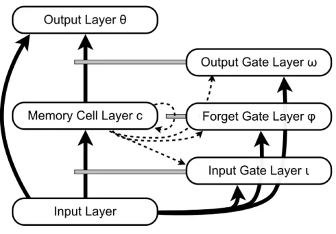
The LSTM network ostensibly has only three layers: an input layer, a layer of memory block cell assemblies, and an output layer. For expository purposes, however, it will be useful to think of the memory block assemblies as composed of multiple separate layers (see Fig. 2): the input gate layer (◆), the forget gate layer ('), the memory cell layer (c), and the output gate layer (!). For notational simplicity, we will stipulate that each of these layers has the same number of elements, implying that a single memory cell cj is associated with
the set of gates ◆j, 'j, and !j; it is trivial to generalize to the case where a
set of gates can control more than one memory cell. The input layer projects a full set of connections to each of these layers; the memory cell layer projects a full set of connections to the output layer (✓). In addition, each memory cell cj projects a single ungated peephole connection to each of its associated gates
(see Fig. 1a). The architecture can be augmented with direct input-to-output connections and/or delayed recurrent connections among the memory cell and gate layers. As will become evident in the following sections, the operation of the LSTM training algorithm is very much dependent upon the specific architecture that we have just described.
The following equations detail the operation of the LSTM network through a single time-step. We consider a time-step to consist of the presentation of a single input, followed by the activation of all subsequent layers of the network in order. We think that this notion of a time-step, most often seen when discussing
Me mo ry C el l Pe ep ho le C on ne ct io ns Output Gate Forget Gate Input Gate
(a) LSTM memory block
Me mo ry C el l Pe ep ho le C on ne ct io ns Forget Gate Output Gate Input Gate (b) Equivalent LSTM-g architecture
Figure 1: Architectural comparison of LSTM’s memory block to the equivalent in an LSTM-g network. Weighted connections are shown as black lines, and gating relationships are shown as thicker gray lines. The elongated enclosure represents the extent of the memory cell. In (a), connections into the LSTM memory cell are first summed (the input-squashing function is taken to be the identity); the result is gated by the input gate. The gated net input progresses to the self-recurrent linear unit, whose activity is gated by the forget gate. The state of the recurrent unit is passed through the output-squashing function, which is then modulated by the output gate. This modulated value is passed to all receiving units via weighted connections. Note that the peephole connections project from an internal stage in the memory cell to the controlling gate units; this is an exception to the rule that only the final value of the memory cell is visible to other units. In (b), the weights on the input connections to the LSTM-g memory cell are modulated directly by the input gate before being summed by the linear unit. Unmodulated output leaves the memory cell via weighted connections. Connections to downstream units can have their weights modulated directly by the output gate, but this is not required, as can be seen with the equivalent of LSTM’s peephole connections proceeding normally from the output of the memory cell. This scheme is capable of producing the same results as the LSTM memory block, but allows greater architectural flexibility.
Input Layer
Output Layer
!
Memory Cell Layer c
Forget Gate Layer
"
Output Gate Layer
#
Input Gate Layer
ɩ
Figure 2: The standard LSTM architecture in terms of layers. The memory block assemblies are broken up into separate layers of memory cells, input gates, forget gates, and output gates, in addition to the input and output layers. Solid arrows indicate full all-to-all connectivity between units in a layer, and dashed arrows indicate connectivity only between the units in the two layers that have the same index (i.e., the first unit of the sending layer only projects to the first unit of the receiving layer, the second unit only projects to the second, and so forth). The gray bars denote gating relationships, and are displayed as they are conceived in LSTM-g, with the modulation occurring at the connection level. Units in each gate layer modulate only those connections into or out of their corresponding memory cell. The circular dashed connection on the memory cell layer indicates the self-connectivity of the units therein. This diagram shows the optional peephole connections—the dashed arrows originating at the memory cells and ending at the gate layers—as well as the optional direct input-to-output layer connections on the left.
feed-forward networks, enables a more intuitive description of the activation and learning phases that occur due to each input. Following Graves et al. (2004), all variables in the following refer to the most recently calculated value of that variable (whether during this time-step or the last), with the exception that variables with a hat (b) always refer to the value calculated one time-step earlier; this only happens in cases where the new value of a variable is being defined in terms of its immediately preceding value. Following Gers & Schmidhuber (2000), we deviate from the original description of LSTM by reducing the number of squashing functions for the memory cells; here, however, we omit the input-squashing functiong (equivalent to defining g(x) =x) and retain the output-squashing function, naming itfcj for memory cellj. In general, we will use the subscript indexj to refer to individual units within the layer in question, with irunning over all units which project connections to unitj, andkrunning over all units that receive connections fromj.
2.1. Activation dynamics
When an input is presented, we proceed through an entire time-step, acti-vating each layer in order: ◆,', c,!, and finally the output layer✓. In general, when some layer is activated, each unit j in that layer calculates itsnet input
x j as the weighted sum over all its input connections from unitsi(Eq. 1). The units i vary for each layer and potentially include recurrent connections; the most recent activation value of the sending unit is always used, even if it is from the previous time-step as for recurrent connections. For units that are not in the memory cell layer, the activation y j of the unit is the result of applying the unit’s squashing function f j (generally taken to be the logistic function) to its net input (Eq. 2). Each memory cell unit, on the other hand, retains its previous statesccj in proportion to the activation of the associated forget gate; the currentstate scj is updated by the net input modulated by the activation of the associated input gate (Eq. 3). A memory cell’s state is passed through its squashing function and modulated by the activation of its output gate to produce the cell’s activation (Eq. 4).
x j = X i w jiyi for 2{◆,', c,!,✓} (1) y j =f j(x j) for 2{◆,',!,✓} (2) scj =y'j sccj +y◆jxcj (3) ycj =y!j fcj(scj) (4)
When considering peephole connections in the context of the equations in this section, one should replace the sending unit activationyiwith the memory
cell statesci since peephole connections come directly from the internal state of the memory cells rather than their activations.
2.2. Learning rules
In order to learn e↵ectively, each unit needs to keep track of the activity flow over time through each of its connections. To this end, each unit maintains
an eligibility trace for each of its input connections, and updates this trace
immediately after calculating its activation. The eligibility trace for a given connection is a record of activations that have crossed the connection which may still have influence over the state of the network, and is similar to those used in temporal-di↵erence learning (Sutton & Barto, 1998), except that here eligibility traces do not decay. When a target vector is presented, the eligibility traces are used to help assign error responsibilities to individual connections. For the output gates and output units, the eligibility traces are instantaneous—they are simply the most recent activation value that crossed the connection (Eq. 5). For the memory cells (Eq. 6), forget gates (Eq. 7), and input gates (Eq. 8), the eligibility traces are partial derivatives of the state of the memory cell with respect to the connection in question; simplifying these partial derivatives results in Eqs. 6–8. Previous eligibility traces are retained in proportion to the amount of state that the memory cell retains (i.e., the forget gate activationy'j), and each is incremented according to the e↵ect it has on the memory cell state.
" ji=yi for 2{!,✓} (5)
"cji=y'j d"cji+y◆jyi (6) "'ji=y'j "d'ji+sccjf'0j(x'j)yi (7) "◆ji=y'j d"◆ji+xcjf◆0j(x◆j)yi (8) Between time-steps of the activation dynamics (i.e., after the network has generated an output for a given input), the network may be given a target vector tto compare against, where all values intare in the range [0,1]. The di↵erence between the network output and the target is calculated using the cross-entropy function (Eq. 9) (Hinton, 1989). Since E 0 when the t andy values fall in the range [0,1] as we require, one trains the network by driving this function towards zero using gradient ascent. Deriving Eq. 9 with respect to the output unit activations reveals theerror responsibility ✓j for the output units (Eq. 10). One obtains the deltas for the output gates (Eq. 11) and the remaining units (Eq. 12) by propagating the error backwards through the network.
E=X j2✓ tjlog(y✓j) + (1 tj) log(1 y✓j) (9) ✓j =tj y✓j (10) !j =f 0 !j(x!j)fcj(scj) X k2✓ ✓kw✓kcj (11) j =f 0 cj(scj)y!j X k2✓ ✓kw✓kcj for 2{◆,', c} (12)
Finally, the connection weights into all units in each layer are updated according to the product of the learning rate↵, the unit’s error responsibility
j, and the connection’s eligibility trace" ji (Eq. 13).
w ji=↵ j " ji for 2{◆,', c,!,✓} (13)
3. Generalized LSTM
The Long Short Term Memory algorithm, as presented in Section 2, is an efficient and powerful recurrent neural network training method, but is lim-ited in applicability to the architecture shown in Fig. 2 and sub-architectures thereof1. In particular, any architectures with multiple hidden layers (where
another hidden layer projects to the memory block layer) cannot be efficiently trained because error responsibilities are truncated at the memory blocks in-stead of being passed to upstream layers. This section details our generalized version of LSTM, which confers all the benefits of the original algorithm, yet can be applied without modification to arbitrary second-order neural network architectures.
With the Generalized Long Short-Term Memory (LSTM-g) approach, the gating mechanism employed by LSTM is reinterpreted. In LSTM, gate units directly act on the states of individual units—a memory cell’s net input in the case of the input gate, the memory cell state for the forget gate, and the mem-ory cell output for the output gate (Eqs. 3–4). By contrast, units in LSTM-g can gate at the level of individual connections. The e↵ect is that, when passing activity to unitj from unit iacross a connection gated by k, the result is not simplywjiyi, but instead wjiyiyk. In this sense, LSTM-g is similar in form
to traditional second-order networks (e.g., Giles & Maxwell, 1987; Psaltis et al., 1988; Shin & Ghosh, 1991; Miller & Giles, 1993), but with an asymmetry: Our notation considers the connection in this example to be primarily defined by j andi (note that the weight is denoted wji and notwjki), where k provides
a temporarygain on the connection by modulating its weight multiplicatively. This notation is convenient when considering connections which require an out-put and an inout-put, but may or may not be gated; in other words, we can refer to a connection without knowing whether it is a first- or second-order connection. In LSTM-g, every unit has the potential to be like LSTM’s memory cells, gate units, both, or neither. That is to say, all units contain the same set of operating instructions for both activation and learning. Self-connected units can retain state like a memory cell, and any unit can directly gate any connection. The role each unit takes is completely determined by its placement in the overall network architecture, leaving the choice of responsibilities for each unit entirely up to the architecture designer.
1LSTM can also train architectures with additional layers that operate inparallel with the memory block layer, but the important point here is that LSTM cannot e↵ectively train architectures containing layers that operate inserieswith the memory block layer.
Equations 14–24 describe the operation of LSTM-g networks through a single time-step. Just as in our description of LSTM, a time-step consists of the presentation of a single input pattern, followed by the ordered activation of all non-input layers of the network. The order in which layers are activated is pre-determined and remains fixed throughout training. If a layer to be activated receives recurrent connections from a layer which has not yet been activated this time-step, the sending layer’s activations from the previous time-step are used. The full derivation of the LSTM-g training algorithm can be found in Appendix A.
3.1. Activation dynamics
LSTM-g performs LSTM-like gating by having units modulate the e↵ ective-ness of individual connections. As such, we begin by specifying thegain gjion
the connection from unitito unitj (Eq. 14). gji=
⇢ 1 if connection from
itoj is not gated
yk if unitkgates the connection fromito j (14)
Much as with memory cells in LSTM, any unit in an LSTM-g network is capable of retaining state from one time-step to the next, based only on whether or not it is self-connected. The state sj of a unitj (Eq. 15) is the sum of the
weighted, gated activations of all the units that project connections to it. If the unit is self-connected it retains its state in proportion to the gain on the self-connection. As in LSTM, self-connections in LSTM-g, where they exist, have a fixed weight of 1; otherwisewjj = 0. Given the statesj, the activation
yj is calculated via the application of the unit’ssquashing functionfj (Eq. 16).
sj=gjjwjjsbj+
X
i6=j
gjiwjiyi (15)
yj=fj(sj) (16)
When considering these equations as applied to the LSTM architecture, for a unitj /2cwe can see that Eq. 15 is a generalization of Eq. 1. This is because the first term of Eq. 15 evaluates to zero on this architecture (since there is no self-connectionwjj), and all thegji= 1 since no connections into the unit are
gated. The equivalence of Eq. 16 and Eq. 2 for these units follows immediately. For a memory cellj 2c, on the other hand, Eq. 15 reduces to Eq. 3 when one notes that the self-connection gaingjjis justy'j, the self-connection weightwjj is 1, and thegji are all equal to y◆j and can thus be pulled outside the sum. However, for the memory cell units, Eq. 16 is not equivalent to Eq. 4, since the latter already multiplies in the activationy!j of the output gate, whereas this modulation is performed at the connection level in LSTM-g.
3.2. Learning rules
As in LSTM, each unit keeps an eligibility trace "ji for each of its input
this connection has influenced the current state of the unit, and is equal to the partial derivative of the state with respect to the connection weight in question (see Appendix A). For units that do not have a self-connection, the eligibility trace "ji reduces to the most recent input activation modulated by the gating
signal.
"ji=gjjwjj"cji+gjiyi (17)
In the context of the LSTM architecture, Eq. 17 reduces to Eq. 5 for the output gates and output units; in both cases, the lack of self-connections forces the first term to zero, and the remaininggjiyi term is equivalent to LSTM’syi.
If unit j gates connections into other units k, it must maintain a set of
extended eligibility traces "k
ji for each such k (Eq. 18). A trace of this type
captures the e↵ect that the connection fromipotentially has on the state ofk through its influence onj. Eq. 18 is simpler than it appears, as the remaining partial derivative term is 1 if and only if j gates k’s self-connection, and 0 otherwise. Further, the indexa, by definition, runs over only those units whose connections tokare gated byj; this set of units may be empty.
"kji=gkkwkk"ckji+fj0(sj)"ji 0 @@gkk @yj wkksbk+ X a6=k wkaya 1 A (18) It is worth noting that LSTM uses traces of exactly this type for the forget gates and input gates (Eq. 7–8); it just so happens that each such unit gates connections into exactly one other unit, thus requiring each unit to keep only a single, unified eligibility trace for each input connection. This will be the case for the alternative architectures we explore in this paper as well, but is not required. A complete explanation of the correspondence between LSTM’s eligibility traces and the extended eligibility traces utilized by LSTM-g can be found in Appendix B.
When a network is given a target vector, each unit must calculate its error responsibility j and adjust the weights of its incoming connections accordingly.
Output units, of course, receive their values directly from the environment based on the global error function (Eq. 9), just as in LSTM (Eq. 10). The error responsibility j for any other unit j in the network can be calculated
by back-propagating errors. Since each unit keeps separate eligibility traces corresponding to projected activity ("ji) and gating activity ("kji), we divide the
error responsibility accordingly. First, we definePjto be the set of unitskwhich
are downstream from j—that is, activated afterj during a time-step—and to whichj projects weighted connections (Eq. 19), andGj to be the set of units
k which are downstream fromj that receive connections gated by j (Eq. 20). We restrict both of these sets to downstream units because an upstream unitk has its error responsibility updated afterj during backward error propagation, meaning that the error responsibility information provided bykis not available
whenj would need to use it.
Pj ={k|j projects a connection to kandkis downstream ofj} (19)
Gj ={k|j gates a connection intokandk is downstream ofj} (20)
We first find the error responsibility of unitj with respect to the projected connections inPj (Eq. 21), which is calculated as the sum of the error
respon-sibilities of the receiving units weighted by the gated connection strengths that activity fromj passed over to reach k.
Pj =fj0(sj)
X
k2Pj
kgkjwkj (21)
Since the memory cells in LSTM only project connections and perform no gating themselves, Pj of Eq. 21 translates directly into Eq. 12 for these units, which can be seen by noting that the gain termsgkj are all equal to the output
gate activationy!j and can be pulled out of the sum.
The error responsibility of j with respect to gating activity is the sum of the error responsibilities of each unit k receiving gated connections times a quantity representing the gated, weighted input that the connections provided to k (Eq. 22). This quantity, as with the same quantity in Eq. 18, is simpler than it appears, with the partial derivative evaluating to 1 only whenjis gating k’s self-connection and zero otherwise, and the indexarunning over only those units projecting a connection tokon whichj is the gate.
Gj =fj0(sj) X k2Gj k 0 @@gkk @yj wkksbk+ X a6=k wkaya 1 A (22)
To findj’s total error responsibility (Eq. 23), we add the error responsibilities due to projections and gating.
j = Pj+ Gj (23)
In order to obtain weight-changes similar to LSTM, jis not used directly in
weight adjustments; its purpose is to provide a unified value that can be used by upstream units to calculate their error responsibilities due to unitj. Instead, the weights are adjusted by combining the error responsibilities and eligibility traces for projected activity and adding the products of extended eligibility traces and error responsibilities of each unit receiving gated connections. The result is multiplied by the learning rate↵(Eq. 24).
wji=↵ Pj "ji+↵
X
k2Gj
k"kji (24)
Appendix B provides a detailed derivation that shows that the weight changes made by both the LSTM (Eq. 13) and LSTM-g (Eq. 24) algorithms are identical when used on an LSTM architecture without peephole connections. This establishes that LSTM-g is indeed a generalization of LSTM.
4. Comparison of LSTM and LSTM-g
As stated in Section 3 and proved in Appendix B, an LSTM-g network with the same architecture as an LSTM network will produce the same weight changes as LSTM would, provided that peephole connections are not present. When peephole connections are added to the LSTM architecture, however, LSTM-g utilizes a source of error that LSTM neglects: error responsibilities back-propagated from the output gates across the peephole connections to the associated memory cells, and beyond. To see this, we will calculate the error responsibility for a memory cell j in an LSTM-g network, and compare the answer to LSTM’s prescribed error responsibility for that same unit.
We begin with the generic error responsibility equation from LSTM-g (Eq. 23). Since the cell in question is the architectural equivalent of a memory cell, it performs no gating functions; thus the set of gated cellsGjis empty and Gj is zero, leaving Pj alone as the error responsibility. Substituting Eq. 21 for Pj we obtain Eq. 25. At this point we ask: Which units are in Pj? The memory cell in question projects connections to all the output units and sends peephole connections to its controlling input gate, forget gate, and output gate. From this set of receiving units, only the output units and the output gate are downstream from the memory cell, so they comprisePj. Taking each type of
unit inPj individually, we expand the sum and obtain Eq. 26. Finally, we
rec-ognize that the peephole connection to the output gate is not gated, so theg!jcj term goes to 1 (by Eq. 14); in addition, all the output connections are gated by the output gate, so everyg✓kcj term becomesy!j, and we can pull the term outside the sum.
j= Pj =f 0 cj(scj) X k2Pj kgkjwkj (25) =fc0j(scj) X k2✓ ✓kg✓kcjw✓kcj+ !jg!jcjw!jcj ! (26) =fc0j(scj) y!j X k2✓ ✓kw✓kcj + !jw!jcj ! (27) The resulting Eq. 27 should be equal to cj as shown in Eq. 28 (derived from Eq. 12) to make LSTM-g equivalent to LSTM in this case.
cj =f 0 cj(scj)y!j X k2✓ ✓kw✓kcj (28)
Upon inspection, we see that that LSTM-g includes a bit of extra back-propagated error ( !jw!jcj) originating from the output gate. Besides giving a more accurate weight update for connections into memory cellj, this change in error will be captured in j and passed upstream to the forget gates and input
gates. As demonstrated in Section 5, this extra information helps LSTM-g perform a bit better than the original algorithm on an LSTM architecture with peephole connections.
5. Experiments
To examine the e↵ectiveness of LSTM-g, we implemented the algorithm described in Section 3 and performed a number of experimental comparisons using various architectures, with the original LSTM algorithm and architecture as a control comparison.
5.1. Distracted Sequence Recall on the standard architecture
In the first set of experiments, we trained di↵erent neural networks on a task we call the Distracted Sequence Recall task. This task is our variation of the “temporal order” task, which is arguably the most challenging task demon-strated by Hochreiter & Schmidhuber (1997). The Distracted Sequence Recall task involves 10 symbols, each represented locally by a single active unit in an input layer of 10 units: 4target symbols, which must be recognized and remem-bered by the network, 4distractor symbols, which never need to be remembered, and 2promptsymbols which direct the network to give an answer. A single trial consists of a presentation of a temporal sequence of 24 input symbols. The first 22 consist of 2 randomly chosen target symbols and 20 randomly chosen dis-tractor symbols, all in random order; the remaining two symbols are the two prompts, which direct the network to produce the first and second target in the sequence, in order, regardless of when they occurred. Note that the targets may appear at any point in the sequence, so the network cannot rely on their tempo-ral position as a cue; rather, the network must recognize the symbols as targets and preferentially save them, along with temporal order information, in order to produce the correct output sequence. The network is trained to produce no output for all symbols except the prompts, and for each prompt symbol the network must produce the output symbol which corresponds to the appropriate target from the sequence.
The major di↵erence between the “temporal order” task and our Distracted Sequence Recall task is as follows. In the former, the network is required to activate one of 16 output units, each of which represents a possible ordered se-quence of both target symbols. In contrast, the latter task requires the network to activate one of only 4 output units, each representing a single target symbol; the network must activate the correct output unit for each of the targets, in the same order they were observed. Requiring the network to produce outputs in sequence adds a layer of difficulty; however, extra generalization power may be imparted by the fact that the network is now using the same output weights to indicate the presence of a target, regardless of its position in the sequence. Because the “temporal order” task was found to be unsolvable by gradient train-ing methods other than LSTM (Hochreiter & Schmidhuber, 1997), we do not include methods other than LSTM and LSTM-g in the comparisons.
Our first experiment was designed to examine the impact of the extra error information utilized by LSTM-g. We trained two networks on the Distracted Sequence Recall task. The first network serves as our control and is a typical LSTM network with forget gates, peephole connections, and direct input-to-output connections (see Fig. 2), and trained by the LSTM algorithm. The
second network has the same architecture as the first, but is trained by the LSTM-g algorithm, allowing it to take advantage of back-propagated peephole connection error terms.
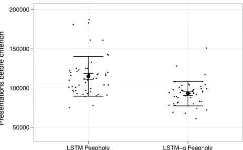
All runs of each network used the same basic approach and parameters: one unit in the input layer for each of the 10 input symbols, 8 units in the memory cell layer and associated gate layers, 4 units in the output layer for the target symbols, and a learning rate↵= 0.1. Both networks are augmented with peep-hole connections and direct input-to-output connections. Thus, both algorithms are training networks with 416 weights. Networks were allowed to train on ran-dom instances of the Distracted Sequence Recall task until they achieved the performance criterion of 95% accuracy on a test set of 1000 randomly selected sequences which the network had never encountered during training. To get credit for processing a sequence correctly, the network was required to keep all output units below an activation level of 0.5 during all of the non-prompt sym-bols in the sequence and activate only the correct target symbol—meaning that all units must have activations on the same side of 0.5 as the target—for both prompts. This correctness criterion was used for both the LSTM and LSTM-g networks to ensure that the two types were compared on an equal footing. Each network type was run 50 times using randomized initial weights in the range [ 0.1,0.1).
Fig. 3 compares the number of presentations required to train the two net-works. All runs of both networks reached the performance criterion as expected, but there were di↵erences in how quickly they achieved this. In particular, LSTM-g is able to train the LSTM network architecture significantly faster than the original algorithm (as evaluated by a Welch two-sample t-test after removing outliers greater than 2 standard deviations from the sample mean, witht⇡5.1, df ⇡80.9, p <10 5). This demonstrates that LSTM-g can provide
a clear advantage over LSTM in terms of the amount of training required, even on an LSTM-compatible architecture.
5.2. Distracted Sequence Recall on a customized LSTM-g architecture
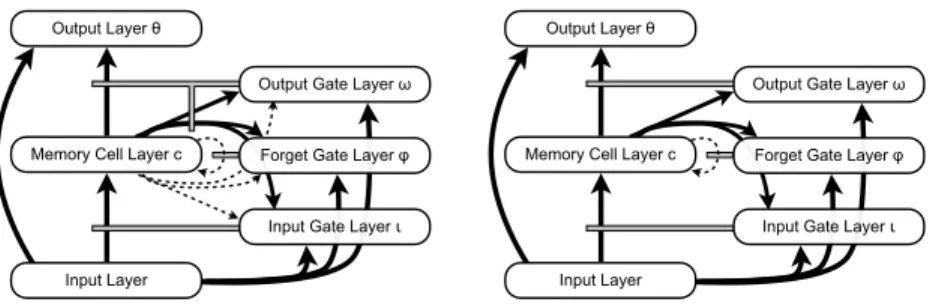
Our second experiment was designed to investigate the relative performance of the standard LSTM architecture compared to other network architectures that do not make sense in the LSTM paradigm. We trained three additional networks on the same Distracted Sequence Recall task. The first serves as the control and utilizes the LSTM algorithm to train a standard LSTM architecture that is the same as in the previous experiment except for the addition of recur-rent connections from all (output-gated) memory cells to all the gate units. We call this architecture the gated recurrence architecture (Fig. 4a). The second network also uses the gated recurrence architecture, but is trained by LSTM-g. The third network is a new ungated recurrence architecture (Fig. 4b), which starts with the standard LSTM architecture and adds direct, ungated connec-tions from each memory cell to all gate units. These connecconnec-tions come from the ungated memory cell output like peephole connections would, but unlike peep-hole connections these are projected to gate units both inside and outside of the local memory block. The intuition behind this architecture comes from the idea
Presentations bef ore cr iter ion 50000 100000 150000 200000 ● ● ● ● ● ● ● ● ● ● ● ● ● ● ● ● ● ● ● ● ● ● ● ● ● ● ● ● ● ● ● ● ● ● ● ● ● ● ● ● ● ● ● ● ● ● ● ● ● ● ● ● ● ● ● ● ● ● ● ● ● ● ● ● ● ● ● ● ● ● ● ● ● ● ● ● ● ● ● ● ● ● ● ● ● ● ● ● ● ● ● ● ● ● ● ● ● LSTM Peephole LSTM−g Peephole
Figure 3: Plot of the results of an experiment that pitted LSTM-g against LSTM, each training an identical standard peephole LSTM architecture to perform the Distracted Sequence Recall task. Small points are individual network runs, jittered to highlight their density. The large black point for each network type is the mean over all 50 runs, with standard error (small bars) and standard deviation (large bars). The results show clearly the beneficial impact of the way LSTM-g utilizes extra error information.
that a memory cell should be able to communicate its contents not only to its controlling gates but also to the other memory blocks in the hidden layer, while still hiding these contents from downstream units. Such communication would intuitively be a major boon for sequential storage and retrieval tasks because it allows a memory block to choose what to store based on what is already stored in other blocks, even if the contents of those blocks are not yet ready to be considered in calculating the network output. These ungated cell-to-gate con-nections are a direct generalization of peephole concon-nections, which, since they extended from an internal state of a memory cell, were already an anomaly in LSTM. Peephole connections were justified in LSTM based on their locality within a single memory block; such locality does not exist for the connections in the ungated recurrence architecture, and therefore training the architecture with LSTM does not make sense. As such, we present only the results of train-ing the ungated recurrence architecture with LSTM-g, which requires no special treatment of these ungated cell-to-gate connections
Each of the three networks uses the same approach and parameters as in the previous experiment. This means the both types of network using the gated recurrence architecture have 608 trainable connections, and the ungated recur-rence architecture has only 584 because the 24 peephole connections used in the
Input Layer Output Layer !
Memory Cell Layer c Forget Gate Layer "
Output Gate Layer #
Input Gate Layer ɩ
(a) Gated recurrence architecture
Input Layer Output Layer !
Memory Cell Layer c Forget Gate Layer "
Output Gate Layer #
Input Gate Layer ɩ
(b) Ungated recurrence architecture
Figure 4: The network architectures used in the second experiment (c.f. Fig. 2). In (a), the previous LSTM architecture is augmented with a full complement of recurrent connec-tions from each memory cell to each gate, regardless of memory block associaconnec-tions; all these connections are gated by the appropriate output gate. In (b), we strip the (now redundant) peephole connections from the original architecture and in their place put a full complement of ungated connections from each memory cell to every gate. This second architectural vari-ant is incompatible with the LSTM training algorithm, as it requires all connections out of the memory cell layer to be gated by the output gate. The network can still be trained by LSTM-g, however.
gated recurrence architecture would be redundant2.
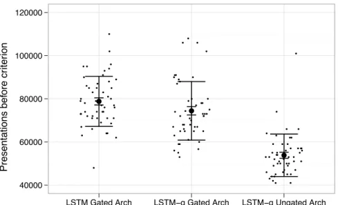
Though these networks are more complex than those in the first experi-ment, they are able to learn the task more quickly. Fig. 5 shows, for each run, the number of input presentations necessary before each of three net-works reached the performance criterion. Again we see a slight speed advan-tage for LSTM-g over LSTM when applied to the LSTM-compatible gated recurrence architecture, though this di↵erence misses statistical significance (t⇡1.8, df ⇡87.9, p <0.08). More interesting is the improvement that LSTM-g achieves on the novel ungated recurrence architecture, which reaches significance easily compared to both the gated recurrence architecture trained with LSTM (t ⇡ 15.3, df ⇡ 79.6, p < 10 15) and with LSTM-g (t
⇡ 10.2, df ⇡ 69.6, p < 10 14). LSTM-g is able to train the ungated recurrence architecture faster than
either it or LSTM train the gated recurrence architecture. This di↵erence illus-trates the potential benefits of the wide range of customized architectures that LSTM-g can train.
5.3. Language Understanding on a two-stage LSTM-g architecture
For our final experiment we adopt a more involved and substantially di↵ er-ent Language Understanding task, similar to those studied recer-ently using other
2The experiments reported here were also run with a variant of the gated recurrence ar-chitecture without the 24 peephole connections, leaving it with the same 584 weights as the ungated recurrence architecture; however, the lack of peephole connections caused a severe learning slowdown. In the interest of comparing LSTM-g against the strongest possible control, we report only the results from the gated recurrence architecture with peephole connections as described above.
Presentations bef ore cr iter ion 40000 60000 80000 100000 120000 ● ● ● ● ● ● ● ● ● ● ● ● ● ● ● ● ● ● ● ● ● ● ● ● ● ● ● ● ● ● ● ● ● ● ● ● ● ● ● ● ● ● ● ● ● ● ● ● ● ● ● ● ● ● ● ● ● ● ● ● ● ● ● ● ● ● ● ● ● ● ● ● ● ● ● ● ● ● ● ● ● ● ● ● ● ● ● ● ● ● ● ● ● ● ● ● ● ● ● ● ● ● ● ● ● ● ● ● ● ● ● ● ● ● ● ● ● ● ● ● ● ● ● ● ● ● ● ● ● ● ● ● ● ● ● ● ● ● ● ● ● ● ● ● ● ● ● ● ● ● ●
LSTM Gated Arch LSTM−g Gated Arch LSTM−g Ungated Arch
Figure 5: Plot of the results on the Distracted Sequenced Recall task for three networks: an LSTM network augmented with peephole connections and gated recurrent connections from all memory cells to all gates; and an LSTM-g network with ungated recurrent connections from all memory cells to all gates. The graph clearly shows that the ungated recurrence network, trainable only with LSTM-g, reaches the performance criterion after less training than the comparable gated recurrence network as trained by either LSTM or LSTM-g.
neural network models (Monner & Reggia, 2009). In this task, a network is given an English sentence as input and is expected to produce a set of predi-cates that signifies the meaning of that sentence as output. The input sentence is represented as a temporal sequence of phonemes, each of which is a vector of binary auditory features, borrowed directly from Weems & Reggia (2006). The network should produce as output a temporal sequence of predicates which bind key concepts in the sentence with their referents. For example, for the input sentence “the red pyramid is on the blue block” we would expect the network to produce the predicatesred(X),pyramid(X),blue(Y),block(Y), andon(X, Y). The variables are simply identifiers used to associate the various predicates
with each other; in this example, the three predicates in which variableX
partic-ipates come together to signify that a single object in the world is a red pyramid which is on top of something else. In the actual output representation used by the network, each predicate type is represented as a single one in a vector of zeroes, and the variables required by each prediate are also represented in this way. In other words, a network performing this task requires a set of output neurons to represent the types of predicates, with each unit standing for a sin-gle predicate type, and two additional, independent sets of neurons which each represent a variable, since there can be at most two variables involved in any
predicate. We chose to require the network to produce the required predicates in a temporal fashion to avoid imposing architectural limits on the number of predicates that a given input sentence could entail.
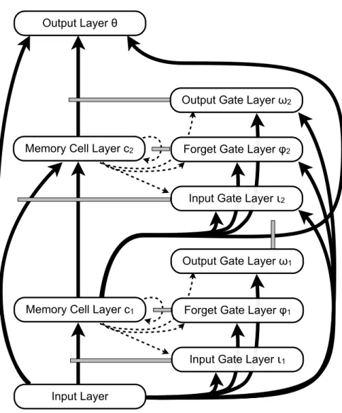
We chose to examine this task in part because it is hierarchically decom-posable. To come up with a readily generalizable solution, common wisdom suggests that the best strategy for the network to use is to aggregate the incom-ing phonemes into words, words into phrases, and phrases into a unified sentence meaning. Our intuition was that architectures capable of directly supporting this type of hierarchical decomposition would be superior to those that do not. To test this notion, we developed an architecture that we call thetwo-stage ar-chitecture, shown in Fig. 6. At first it may appear complex, but it is essentially the standard LSTM architecture with peephole connections, except with a sec-ond hidden layer of memory block assemblies in series with the first. LSTM cannot efficiently train such an architecture, because the back-propagated error signals would be truncated and never reach the earlier layer of memory blocks. LSTM-g, on the other hand, trains the two-stage architecture without difficulty. As a control to our LSTM-g-trained two-stage architecture, we train a standard LSTM network with peephole connections (see Fig. 2) appropriately adjusted to match the resources of the two-stage network as closely as possible.
Both networks in this experiment use essentially the same parameters as in the previous two experiments; the only di↵erence is in the size of the networks. The two-stage architecture has 34 input units (corresponding to the size of the phoneme feature vectors used as input), 40 memory blocks in the first stage, 40 additional memory blocks in the second stage, and 14 output units, giving a total of 13,676 trainable connections. The standard LSTM control has the same 34 input units and 14 output units, with a single hidden layer of 87 memory blocks, giving it a slight edge with 7 more total memory blocks and 13,787 trainable connections. These numbers were selected to give the two networks as near to parity in terms of computational resources as the architecture designs and problem constraints allow.
During a single trial in the Language Understanding task, the network being tested is given each individual phoneme from a sentence as input in consecutive time-steps, and after the entire input sequence has been processed, the network must output one complete predicate on each subsequent time-step, until the network produces a special “done” predicate to signify that it is finished pro-ducing relevant predicates. The networks are trained to produce the predicates for a given sentence in a specified order, but are scored in such a way that cor-rect predicates produced in any order count as corcor-rect answers. A predicate is deemed to be correct if all units have activations on the correct side of 0.5. We also tracked the number of unrelated predicates that the networks generated; however, we found this number to closely track the inverse of the fraction of correct predicates produced, and as such, we only report the latter measure.
A small, mildly context-sensitive grammar was used to generate the sen-tences and corresponding predicates for this simple version of the Language Understanding task. The sentences contained combinations of 10 di↵erent words suggesting meanings involving 8 di↵erent types of predicates with up to 3
dis-Input Layer
Output Layer !
Memory Cell Layer c
1Memory Cell Layer c
2Forget Gate Layer "
2Output Gate Layer #
2Input Gate Layer
ɩ2
Forget Gate Layer "
1Output Gate Layer #
1Input Gate Layer
ɩ1
Figure 6: The two-stage network architecture, used in the third experiment. This architecture is a variant of the standard LSTM architecture with peephole connections (Fig. 2) that has a second layer of memory block assemblies in series with the first. The traditional LSTM training algorithm cannot e↵ectively train this architecture due to the truncation of error signals, which would never reach the earlier layer of memory blocks. Intuition suggests that the two self-recurrent layers allow this network to excel at hierarchically decomposable tasks such as the Language Understanding task.
tinct objects referenced per sentence. The simplest sentences required only 3 output predicates to express their meanings, while the most complex required the networks to produce as many as 9 predicates in sequence as output. Each network was run 32 times on this task. On each run, the network in question began with random weights and was allowed to train through 1 million sentence presentations. The performance of the network was gauged periodically on a battery of 100 test sentences on which the network never received training. The duration of training was more than sufficient to ensure that all networks had reached their peak performance levels.
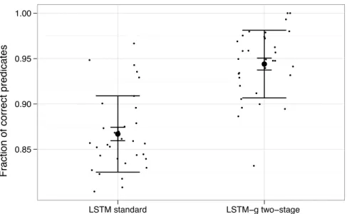
Fig. 7 shows a comparison of the peak performance rates of the two types of network, based on the fraction of correct predicates produced on the novel test sentences. The two-stage network trained with LSTM-g was able to achieve sig-nificantly better generalization performance than the standard LSTM network on average (t ⇡ 9.4, df ⇡ 57.9, p < 10 12). In addition, the two-stage
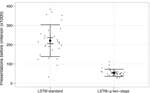
net-work was able to achieve this performance much more quickly than the control. Fig. 8 plots the number of sentence presentations required for each network to produce 80% of predicates correctly; this number was chosen because every run of every network was able to achieve this performance level. The two-stage net-work required approximately 4 times fewer sentence presentations to reach the 80% performance criterion, which is a significant di↵erence (t⇡10.9,df ⇡31.4, p <10 11). These results underscore the value of using LSTM-g to train
cus-tomized architectures that traditional LSTM cannot.
6. Discussion
The original LSTM algorithm was an important advance in gradient training methods for recurrent neural networks that allows networks to learn to handle temporal input and output series, even across long time lags. Until now, how-ever, this algorithm was limited in scope to a small family of second-order re-current neural architectures. This paper has introduced LSTM-g, a generalized algorithm that provides the power and speed of the LSTM algorithm, but un-like LSTM is applicable to arbitrary second-order recurrent neural networks. In addition to the increased architectural applicability it provides, LSTM-g makes use of extra back-propagated error when applied to the canonical LSTM network architecture with peephole connections. We found that this error can be put to good use, with LSTM-g converging after less training than the LSTM training algorithm required in experiments which utilize the standard LSTM network architecture. Further, we found that customized network architectures trained with LSTM-g can produce better performance than either LSTM or LSTM-g can produce when restricted to the standard architecture. In light of previ-ous research that shows LSTM to outperform other recurrent network training algorithms of comparable computational complexity (Hochreiter & Schmidhu-ber, 1997), the results contained herein suggest that LSTM-g may find fruitful application in many areas where non-standard network architectures may be desirable. We conclude that LSTM-g has the potential to both improve the
per-Fr
action of correct predicates
0.85 0.90 0.95 1.00 ● ● ● ● ● ● ● ● ● ● ● ● ● ● ● ● ● ● ● ● ● ● ● ● ● ● ● ● ● ● ● ● ● ● ● ● ● ● ● ● ● ● ● ● ● ● ● ● ● ● ● ● ● ● ● ● ● ● ● ● ● ● ● ● ● ●
LSTM standard LSTM−g two−stage
Figure 7: Plot of the performance results on the Language Understanding task produced by a standard LSTM network and the two-stage architecture trained by LSTM-g. We see that the standard LSTM networks were able to produce approximately 87% of predicates correctly at peak performance, while the two-stage LSTM-g networks garnered 94% on average.
Presentations bef ore cr iter ion (x1000) 0 100 200 300 400 ● ● ● ● ● ● ● ● ● ● ● ● ● ● ● ● ● ● ● ● ● ● ● ● ● ● ● ● ● ● ● ● ● ● ● ● ● ● ● ● ● ● ● ● ● ● ● ● ● ● ● ● ● ● ● ● ● ● ● ●● ● ● ●
LSTM standard LSTM−g two−stage
Figure 8: Plot of the training duration required for each type of network to reach the criterion of producing 80% of the required predicates for input sentences. The standard LSTM net-work required an average of about 220,000 sentence presentations to reach this performance criterion, while the two-stage network trained by LSTM-g required fewer than 60,000.
formance and broaden the applicability of the LSTM family of gradient-based training algorithms for recurrent neural networks.
References
Elman, J. L. (1990). Finding structure in time. Cognitive Science,14, 179–211. Gers, F. A., & Cummins, F. (2000). Learning to forget: Continual prediction
with LSTM. Neural Computation, 12, 2451–2471.
Gers, F. A., P´erez-Ortiz, J. A., Eck, D., & Schmidhuber, J. (2003). Kalman filters improve LSTM network performance in problems unsolvable by tradi-tional recurrent nets. Neural Networks,16, 241–250.
Gers, F. A., & Schmidhuber, J. (2000). Recurrent nets that time and count. In
Proceedings of the International Joint Conference on Neural Networks (pp.
189–194).
Gers, F. A., & Schmidhuber, J. (2001). LSTM recurrent networks learn simple context-free and context-sensitive languages. IEEE Transactions on Neural Networks,12, 1333–1340.
Giles, C. L., & Maxwell, T. (1987). Learning, invariance, and generalization in high-order neural networks. Applied Optics,26, 4972–4978.
Graves, A., Eck, D., Beringer, N., & Schmidhuber, J. (2004). Biologically plausi-ble speech recognition with LSTM neural nets. InProceedings of the Interna-tional Workshop on Biologically Inspired Approaches to Advanced Information
Technology (pp. 127–136).
Hinton, G. E. (1989). Connectionist learning procedures.Artificial Intelligence,
40, 185–234.
Hochreiter, S., & Schmidhuber, J. (1997). Long short-term memory. Neural
Computation,9, 1735–1780.
Miller, C. B., & Giles, C. L. (1993). Experimental comparison of the e↵ect of order in recurrent neural networks. Pattern Recognition,7, 849–872.
Monner, D., & Reggia, J. A. (2009). An unsupervised learning method for representing simple sentences.2009 International Joint Conference on Neural
Networks, (pp. 2133–2140).
Psaltis, D., Park, C., & Hong, J. (1988). Higher order associative memories and their optical implementations. Neural Networks,1, 149–163.
Shin, Y., & Ghosh, J. (1991). The pi-sigma network: An efficient higher-order neural network for pattern classification and function approximation. In
Pro-ceedings of the International Joint Conference on Neural Networks (pp. 13–
Sutton, R. S., & Barto, A. G. (1998). Temporal-di↵erence learning. In
Rein-forcement Learning: An Introduction (pp. 167–200). MIT Press.
Weems, S. A., & Reggia, J. A. (2006). Simulating single word processing in the classic aphasia syndromes based on the Wernicke-Lichtheim-Geschwind theory. Brain and language, 98, 291–309.
Werbos, P. J. (1990). Backpropagation through time: What it does and how to do it. Proceedings of the IEEE,78, 1550–1560.
Williams, R. J., & Zipser, D. (1989). A learning algorithm for continually running fully recurrent neural networks. Neural Computation,1, 270–280.
Appendix A. Learning rule derivation
Here we derive the LSTM-g learning algorithm by calculating the gradient of the cross-entropy function (Eq. 9) for a general unit in an LSTM-g network. Such a unit may both project normal weighted connections to other units and multiplicatively modulate the weights of other connections. In order to know the error responsibility for unitj, we must approximate the gradient of the error function with respect to this unit’s statesj (Eq. A.1). To do this, we begin with
the approximation that the error responsibility of unitjdepends only upon units k which are immediately downstream from j (Eq. A.2). The remaining error gradients forkare k by definition. We break up the second partial derivative
into a product which includes j’s activation directly so as to account for the e↵ects of j’s squashing function separately (Eq. A.3). The dependence of j’s activation on its state is simply the derivative of the squashing function, which is constant across the sum and thus can be moved outside (Eq. A.4). At this point, we can separate our set of units k into two (possibly overlapping) sets (Eq. A.5)—those units to whichj projects weighted connections (Eq. 19), and those units that receive connections gated byj (Eq. 20). We will thus handle error responsibilities for projection and gating separately, even in cases wherej both projects and gates connections into the same unitk, thereby defining Pj and Gj (Eq. A.6, cf. Eq. 23).
j= @E @sj (A.1) ⇡X k @E @sk @sk @sj (A.2) =X k k @sk @yj @yj @sj (A.3) =fj0(sj) X k k @sk @yj (A.4) =fj0(sj) X k2Pj k @sk @yj +fj0(sj) X k2Gj k @sk @yj (A.5)
= Pj + Gj (A.6) In calculating Pj (Eq. A.7), we expandsk using its definition from Eq. 15 to obtain Eq. A.8. Recall that we are only concerned with cases wherej projects connections; as such,gkk andgkj0 do not depend on j and are treated as
con-stants. Since the previous state ofkdoes not depend on the current activation ofj, the first term in the parentheses vanishes completely. Individual terms in the sum vanish as well, except for the one case when j0 = j, leaving us with
gkjwkj for the entire derivative (Eq. A.9, cf. Eq. 21).
Pj =f 0 j(sj) X k2Pj k@sk @yj (A.7) =fj0(sj) X k2Pj k @ @yj 0 @gkkwkksbk+ X j06=k gkj0wkj0yj0 1 A (A.8) =fj0(sj) X k2Pj kgkjwkj (A.9)
As above, to find Gj (Eq. A.10) we first expandsk(Eq. A.11). In this case, we are considering only connections whichj gates. Now thegkkterm is in play,
since it is equal toyj ifjgatesk’s self-connection (see Eq. 14); this leads to the
first term inside the parentheses in Eq. A.12, where the derivative can takes the values 1 or 0. For individual terms in the sum, we knowyj0 6=yj since we are
not dealing with connectionsj projects tok. However,gkj0 may be equal to yj
in some cases; where it is not,jdoes not gate the connection and the term goes to zero. Thus, in Eq. A.12 (cf. Eq. 22), the sum is reindexed to include only those unitsawhose connections tokare gated by j.
Gj =fj0(sj) X k2Gj k@sk @yj (A.10) =fj0(sj) X k2Gj k @ @yj 0 @gkkwkksbk+ X j06=k gkj0wkj0yj0 1 A (A.11) =fj0(sj) X k2Gj k 0 @@gkk @yj wkksbk +X a6=k wkaya 1 A (A.12)
We can now calculate the error responsibility j of any unit j by
back-propagation. We start at the level of unitskthat are immediately downstream fromj (Eq. A.13). We can separate thek units by function again (Eq. A.14), and break up the remaining partial derivative in the first sum (Eq. A.15). Re-arranging terms in the first sum (Eq. A.16), we see a grouping which reduces to
Pj (see Eq. A.7). The remaining derivative in the first term is, by definition, the familiar eligibility trace"ji; in the second term we find the definition of the
extended eligibility trace"k
ji, leaving us with Eq. A.17 (cf. Eq. 24).
wji⇡↵ X k @E @sk @sk @wji (A.13) =↵X k2Pj k @sk @wji +↵X k2Gj k @sk @wji (A.14) =↵X k2Pj k @sk @yj @yj @sj @sj @wji +↵X k2Gj k @sk @wji (A.15) =↵ 0 @fj0(sj) X k2Pj k@sk @yj 1 A @sj @wji +↵X k2Gj k @sk @wji (A.16) =↵ Pj "ji+↵ X k2Gj k"kji (A.17)
To calculate the eligibility trace"ji(Eq. A.18) we simply substitutesj from
Eq. 15 to obtain Eq. A.19. We assume unit j does not gate its own self-connection, sogjjis a constant. The previous statesbjdepends onwjiproducing
a partial derivative that simplifies to the previous value of the eligibility trace,
c
"ji. The only term in the sum with a non-zero derivative is the case where
i0=i, leaving us with Eq. A.20 (cf. Eq. 17).
"ji= @sj @wji (A.18) = @ @wji 0 @gjjwjjsbj+ X i06=j gji0wji0yi0 1 A (A.19) =gjjwjj"cji+gjiyi (A.20)
Working on the extended eligibility trace"k
ji(Eq. A.21), we again expandsk
to form Eq. A.22. Performing the partial derivative on the first term, note that gkk may be equal toyj, which depends onwji; also,sbk depends onwji via its
e↵ect onsj, so we require the product rule to derive the first term. For terms in
the sum, unitj can gate the connection fromj0 to k, butk6=j so w
kj0 can be
treated as constant, as canyj0 since we are not concerned here with connections
thatj projects forward. In Eq. A.23, we are left with the result of the product rule and the remaining terms of the sum, where theaindex runs over only those connections intok that j does in fact gate. Moving to Eq. A.24, we note that the first partial derivative is simply the previous value of the extended eligibility trace. We pull out partial derivatives common to the latter two terms, finally replacing them in Eq. A.25 (cf. Eq. 18) with the names of their stored variable forms. The partial derivatives in the sum are all 1 by the definition of the aindex. The remaining partial derivative inside the parentheses reduces to 1
whenj gatesk’s self-connection and 0 otherwise. "kji= @sk @wji (A.21) = @ @wji 0 @gkkwkksbk+ X j06=k gkj0wkj0yj0 1 A (A.22) =gkkwkk @sbk @wji +@gkk @wji wkksbk+ X a6=k @gka @wji wkaya (A.23) =gkkwkk"ckji+ @yj @sj @sj @wji 0 @@gkk @yj wkksbk+ X a6=k @gka @yj wkaya 1 A (A.24) =gkkwkk"ckji+fj0(sj)"ji 0 @@gkk @yj wkksbk+ X a6=k wkaya 1 A (A.25)
Appendix B. LSTM as a special case of LSTM-g
Here we show that LSTM is a special case of LSTM-g in the sense that, when LSTM-g is applied to a particular class of network architectures, the two algorithms produce identical weight changes. To prove that LSTM-g provides the same weight updates as the original algorithm on the LSTM architecture, we first need to precisely articulate which architecture we are considering. For notational simplicity, we will assume that the desired LSTM architecture has only one memory cell per block; this explanation can be trivially extended to the case where we have multiple memory cells per block. The input layer projects weighted connections forward to four distinct layers of units (see Fig. 2), which are activated in the following order during a time-step, just as in LSTM: the input gate layer ◆, the forget gate layer ', the memory cell layer c, and the output gate layer !. Each of these layers has the same number of units; a group of parallel units are associated via the pattern of network connectivity and collectively function like an LSTM memory block. Inputs to each cell in the memory cell layer are gated by the associated input gate unit. The memory cell layer is the only layer in which each unit has a direct self-connection; these each have a fixed weight of 1 and are gated by the appropriate forget gate. A final output layer receives weighted connections from the memory cell layer which are gated by the output gates.
With this simple LSTM network, LSTM-g produces the same weight changes as LSTM. If we add peephole connections to the network, the error responsi-bilities would di↵er, as LSTM-g is able to use error back-propagated from the output gates across these connections, whereas LSTM does not; this is discussed further in Section 4.
Appendix B.1. State and activation equivalence
We begin by demonstrating the equivalence fo the activation dynamics of LSTM and LSTM-g, when the latter is applied to the standard LSTM architec-ture.
Appendix B.1.1. Gate units
First we show that the activation for each gate unit (i.e., for a general unit
j where 2 {◆,',!}) is the same here as it is in LSTM. Starting from the
LSTM-g state definition (Eq. B.1, cf. Eq. 15), we note that the activations of the gate units are stateless because they have no self connections, meaning w j j = 0 and we can drop the first term (Eq. B.2). On this architecture, the only connections into any of the gate units come from the input layer and are ungated, so all the g ji terms are 1 (Eq. B.3). We are left with the definition of the net input to a normal LSTM unit (Eq. B.4, cf. Eq. 1).
s j =g j j w j j scj + X i6=j g jiw jiyi (B.1) =X i6=j g jiw jiyi (B.2) =X i6=j w jiyi (B.3) =x j for 2{◆,',!} (B.4)
Appendix B.1.2. Output units
The situation is similar for the output units ✓j. Starting from the same
LSTM-g state equation (Eq. B.5, cf. Eq. 15), we drop the first term due to lack of output unit self-connections (Eq. B.6). Since the connections into the output units come from the memory cells, each connection is gated by its corresponding output gate (Eq. B.7). We regroup the terms (Eq. B.8) and note that, by Eq. 4, the output gate activation times the LSTM-g memory cell activation gives us the LSTM memory cell activation (Eq. B.9). The result is a equal to the net input of an LSTM output unit (Eq. B.10, cf. Eq. 1).
s✓j =g✓j✓jw✓j✓j sc✓j + X i2c g✓jiw✓jiyi (B.5) =X i2c g✓jiw✓jiyi (B.6) =X i2c y!iw✓jiyi (B.7) =X i2c w✓ji(y!iyi) (B.8) =X i2c w✓jiyci (B.9)
=x✓j (B.10) We have now proved the equivalence of x j in LSTM and s j in LSTM-g for non-memory cells. It follows directly for these units that the activationy j in LSTM is equivalent to the quantity of the same name in LSTM-g (Eq. B.11, cf. Eq. 16), assuming equivalent squashing functionsf j (Eq. B.12, cf. Eq. 2).
y j =f j(s j) (B.11)
=f j(x j) for 2{◆,',!,✓} (B.12)
Appendix B.1.3. Memory cells
Next we demonstrate the equivalence of memory cell states in LSTM and LSTM-g. Starting again from the unit state equation for LSTM-g (Eq. B.13, cf. Eq. 15), we note first that the self-connection weight is fixed at 1 and the self-connection gate is the associated forget gate (Eq. B.14). Next we note that all of the connections coming into the memory cell in question are gated by the memory cell’s associated input gate, sogcji=y◆j8i and we can bring the term outside the sum (Eq. B.15). Finally, we note that the remaining sum is equal to the net (ungated) input to the memory cell, leaving us with the equation for LSTM memory cell states (Eq. B.16, cf. Eq. 3).
scj =gcjcjwcjcj sccj + X i6=cj gcjiwcjiyi (B.13) =y'jsccj+ X i6=cj gcjiwcjiyi (B.14) =y'jsccj+y◆j X i6=cj wcjiyi (B.15) =y'jsccj+y◆j xcj (B.16)
The activation variableycj does not line up directly in LSTM-g and LSTM, since LSTM requires the output gate to modulate the activation of the memory cell directly, while LSTM-g defers the modulation until the activation is passed on through a gated connection. The distinction has already been noted and appropriately dealt with in the discussion of Eq. B.8, and is not problematic for the proof at hand.
Appendix B.2. Weight change equivalence
We have shown the equivalence of activation dynamics when LSTM-g is used on the LSTM architecture. We now must show the equivalence of the weight changes performed by each algorithm.