Market Size, Competition, and the Product Mix of Exporters

(1)

C E N T R E D ’ É T U D E S P R O S P E C T I V E S E T D ’ I N F O R M A T I O N S I N T E R N A T I O N A L E S D O C U M E N T D E T R A V A

Market Size, Competition, and the Product Mix of

Exporters

Thierry Mayer Marc Melitz Gianmarco Ottaviano

(2)

Non-technical Summary

Recent empirical evidence has highlighted how the export patterns of multi-product firms dominate world trade flows, and how these multi-product firms respond to different economic conditions across export markets by varying the number of products they export. In this paper, we further analyze the ef-fects of those export market conditions on the relative export sales of those goods: we refer to this as the firm’s product mix choice. We build a theoretical model of multi-product firms that highlights how mar-ket size and geography (the marmar-ket sizes of and bilateral economic distances to trading partners) affect both a firm’s exported product range and its exported product mix across market destinations. We show how tougher competition in an export market – associated with a downward shift in the distribution of markups across all products sold in the market – induces a firm to skew its export sales towards its best performing products. We find very strong confirmation of this competitive effect for French exporters across export market destinations. Our theoretical model shows how this effect of export market compe-tition on a firm’s product mix then translates into differences in measured firm productivity: when a firm skews its production towards better performing products, it also allocates relatively more workers to the production of those goods and raises its overall output (and sales) per worker. Thus, a firm producing a given set of products with given unit input requirements will produce relatively more output and sales per worker (across products) when it exports to markets with tougher competition. To our knowledge, this is a new channel through which competition (both in export markets and at home) affects firm-level productivity. This effect of competition on firm-level productivity is compounded by another channel that operates through the endogenous response of the firm’s product range: firms respond to increased competition by dropping their worst performing products.

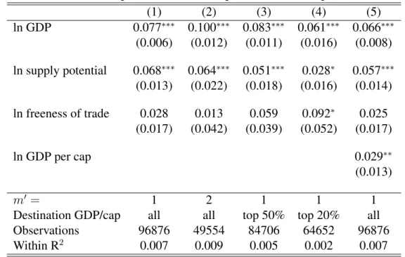
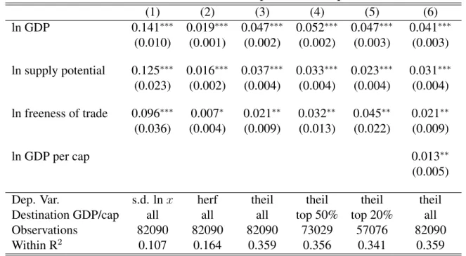
Our empirical results show that country size and supply potential of the destination country (both raising competition intensity in our model) have a strong and highly significant effect on the skewness of export sales, independently of the various measures of skewness we use. These effects are also economically significant. Our coefficients can be directly interpreted as elasticities for the skewness measures with respect to country size and geography. For instance, the elasticity we obtain in our benchmark regression implies that an increase in destination GDP from that of the Czech Republic to German GDP (an increase from the 79th to 99th percentile in the world’s GDP distribution in 2003) would induce French firms to increase their relative exports of their best product (relative to their next best global product) by 42.1%: from an observed mean ratio of 20 in 2003 to 28.4. Those are economically large effects, suggesting an important impact of firms’ productivity too, a topic left for future research.

Abstract

We build a theoretical model of multi-product firms that highlights how market size and geography (the market sizes of and bilateral economic distances to trading partners) affect both a firm’s exported product range and its exported product mix across market destinations (the distribution of sales across products for a given product range). We show how tougher competition in an export market induces a firm to skew its export sales towards its best performing products. We find very strong confirmation of this competitive effect for French exporters across export market destinations. Trade models based on exogenous markups cannot explain this strong significant link between destination market characteristics and the within-firm skewness of export sales (after controlling for bilateral trade costs). Theoretically,

(4)

this within firm change in product mix driven by the trading environment has important repercussions on firm productivity and how it responds to changes in that trading environment.

JEL Classification: F12.

(5)

TAILLE DU MARCHÉ, CONCURRENCE, ET ÉCHELLE DES VENTES DES EXPORTATEURS

Résume non technique

Les études empiriques récentes ont mis en évidence qu’une grande partie des exportations mondiales est effectuée par des entreprises multi-produits qui s’adaptent aux conditions économiques prévalant sur les différents marchés en faisant varier le nombre de produits exportés vers chacun. Dans cet article, nous approfondissons l’analyse des effets de ces caractéristiques des marchés, en considérant la façon dont elles affectent la part des différents produits dans les ventes ; la composition par produits des ventes d’une firme est désignée par le terme “échelle des ventes”. Nous construisons un modèle théorique qui met en évidence comment la taille des marchés et leur éloignement affectent à la fois la gamme (ou nombre) de produits exportés par une entreprise et son échelle des ventes sur chaque marché. Nous montrons com-ment une concurrence plus forte sur un marché d’exportation - qui est associée à des marges plus faibles sur tous les produits vendus - amène la firme à modifier l’échelle de ses ventes en faveur de ses produits les plus performants. Les données d’exportation des entreprises françaises confirment nettement cet ef-fet pro-compétitif. Notre modèle théorique montre comment cet efef-fet de la concurrence sur l’échelle des ventes se transmet à la productivité de l’entreprise : lorsqu’une entreprise concentre sa production sur ses produits les plus performants, elle alloue plus de travailleurs à la production de ces biens et augmente ainsi sa production totale (et ses ventes) par travailleur. Ainsi, pour un ensemble donné de produits et de coûts unitaires de production, une firme réalise des ventes globales par travailleur plus importantes quand elle exporte vers des marchés plus concurrentiels. Nous identifions ainsi un nouveau canal par lequel la concurrence (tant sur les marchés à l’exportation que domestique) affecte la productivité indi-viduelle des entreprises. Cet effet de la concurrence sur la productivité des entreprises est renforcé par un autre canal, celui de la modification endogène de la gamme de produits : les entreprises réagissent à une plus forte concurrence en supprimant de leur gamme les produits les moins performants.

Nos résultats empiriques montrent que la taille et la centralité géographique du pays de destination (deux facteurs qui augmentent l’intensité de la concurrence dans notre modèle) ont un effet important et très significatif sur l’échelle des ventes à l’exportation. Les coefficients estimés peuvent être directement interprétés comme des élasticités de la concentration par produit des ventes par rapport à la taille du pays et à sa géographie. Par exemple, l’élasticité que nous obtenons dans notre régression de référence implique qu’une augmentation du PIB du marché de destination du niveau de la République tchèque à celui du PIB allemand (du 79e au 99e percentile de la distribution mondiale du PIB en 2003) inciterait les entreprises françaises à accroître les ventes relatives de leur meilleur produit de 42% par rapport au produit suivant : il passerait d’une part moyenne de 20% à 28,4%. Ce sont là des effets économiques importants qui suggèrent un impact significatif sur la productivité des firmes, sujet que nous aborderons dans nos recherches à venir.

Résumé court

Nous proposons un modèle théorique de firmes multi-produits qui met en lumière la manière dont la taille du marché de destination et ses caractéristiques géographiques affectent à la fois la gamme des produits exportés et la composition des exportations (pour une gamme donnée). Nous montrons qu’une concurrence forte sur un marché de destination incite les entreprises à concentrer leurs ventes sur leurs meilleurs produits. Nous trouvons une forte confirmation de cet effet pro-concurrentiel chez les exporta-teurs français. Les modélisations existantes du commerce international reposant sur des taux de marges

(6)

exogènes ne peuvent expliquer ce lien important entre les caractéristiques des pays de destination et la concentration des ventes d’un exportateur (une fois prises en compte les barrières commerciales). Sur le plan théorique, nous montrons que ces différences dans la composition des ventes produites par l’environnement commercial ont des répercussions importantes sur la productivité des firmes exportatri-ces.

Classification JEL: F12

(7)

MARKETSIZE, COMPETITION, AND THE PRODUCT MIX OFEXPORTERS1 Thierry Mayer∗ Marc J. Melitz† Gianmarco I.P. Ottaviano‡

1 Introduction

Recent empirical evidence has highlighted how the export patterns of multi-product firms dom-inate world trade flows, and how these multi-product firms respond to different economic con-ditions across export markets by varying the number of products they export.2 _{In this paper, we} further analyze the effects of those export market conditions on the relative export sales of those goods: we refer to this as the firm’s product mix choice. We build a theoretical model of multi-product firms that highlights how market size and geography (the market sizes of and bilateral economic distances to trading partners) affect both a firm’s exported product range and its ex-ported product mix across market destinations. We show how tougher competition in an export market – associated with a downward shift in the distribution of markups across all products sold in the market – induces a firm to skew its export sales towards its best performing products. We find very strong confirmation of this competitive effect for French exporters across export market destinations. Our theoretical model shows how this effect of export market competition on a firm’s product mix then translates into differences in measured firm productivity: when a firm skews its production towards better performing products, it also allocates relatively more workers to the production of those goods and raises its overall output (and sales) per worker. Thus, a firm producing a given set of products with given unit input requirements will produce relatively more output and sales per worker (across products) when it exports to markets with tougher competition. To our knowledge, this is a new channel through which competition (both in export markets and at home) affects firm-level productivity. This effect of competition on firm-level productivity is compounded by another channel that operates through the endoge-nous response of the firm’s product range: firms respond to increased competition by dropping their worst performing products.3

Feenstra and Ma (2008) and Eckel and Neary (2010) also build theoretical models of multi-product firms that highlight the effect of competition on the distribution of firm multi-product sales. Both models incorporate the cannibalization effect that occurs as large firms expand their

prod-1_{We thank Steve Redding, Dan Trefler for helpful comments and suggestions. We are also grateful to seminar}

participants for all the useful feedback we received. Ottaviano thanks Bocconi University, MIUR and the European Commission for financial support. Melitz thanks the Sloan Foundation for financial support. Melitz and Ottaviano thank Sciences Po and CEPII for their hospitality while part of this paper was written.

∗_{Sciences-Po (Paris), CEPII and CEPR (}_{thierry.mayer@sciences-po.fr}₎ †_{Harvard University, NBER and CEPR (}_{mmelitz@harvard.edu}₎

‡_{Bocconi University, FEEM and CEPR (}_{gianmarco.ottaviano@unibocconi.it}_).

2_{See Mayer and Ottaviano (2007) for Europe, Bernard et al (2007) for the U.S., and Arkolakis and Muendler}

(2010) for Brazil.

3_{Bernard et al (forthcoming) and Eckel and Neary (2010) emphasize this second channel. They show how trade}

liberalization between symmetric countries induces firms to drop their worst performing products (a focus on “core competencies”) leading to intra-firm productivity gains. We discuss those papers in further detail below.

(8)

uct range. In our model, we rely on the competition effects from the demand side, which are driven by variations in the number of sellers and their average prices across export markets. The cannibalization effect does not occur as a continuum of firms each produce a discrete number of products and thus never attain finite mass. The benefits of this simplification is that we can consider an open economy equilibrium with multiple asymmetric countries and asymmetric trade barriers whereas Feenstra and Ma (2008) and Eckel and Neary (2010) restrict their anal-ysis to a single globalized world with no trade barriers. Thus, our model is able to capture the key role of geography in shaping differences in competition across export market destinations.4 Another approach to the modeling of multi-product firms relies on a nested C.E.S. structure for preferences, where a continuum of firms produce a continuum of products. The cannibalization effect is ruled out by restricting the nests in which firms can introduce new products. Allan-son and Montagna (2005) consider such a model in a closed economy, while Arkolakis and Muendler (2010) and Bernard et al (forthcoming) develop extensions to open economies. Given the C.E.S. structure of preferences and the continuum assumptions, markups across all firms and products are exogenously fixed. Thus, differences in market conditions or proportional reductions in trade costs have no effect on a firm’s product mix choice (the relative distribution of export sales across products). In contrast, variations in markups across destinations (driven by differences in competition) generate differences in relative exports across destinations in our model: a given firm selling the same two products across different markets will export relatively more of the better performing product in markets where competition is tougher. In our com-prehensive data covering nearly all French exports, we find that there is substantial variation in this relative export ratio across French export destinations, and that this variation is consistently related to differences in market size and geography across those destinations (market size and geography both affect the toughness of competition across destinations).

Theoretically, we show how this effect of tougher competition in an export market on the ex-ported product mix is also associated with an increase in productivity for the set of exex-ported products to that market. We show how firm-level measures of exported output per worker as well as deflated sales per worker for a given export destination (counting only the exported units to a given destination and the associated labor used to produce those units) increase with tougher competition in that destination. This effect of competition on firm productivity holds even when one fixes the set of products exported, thus eliminating any potential effects from the extensive (product) margin of trade. In this case, the firm-level productivity increase is en-tirely driven by the response of the firm’s product mix: producing relatively more of the better performing products raises measured firm productivity. Our model also features a response of the extensive margin of trade: tougher competition in the domestic market induces firms to reduce the set of produced products, and tougher competition in an export market induces exporters to reduce the set of exported products. We do not emphasize these results for the extensive margin, because they are quite sensitive to the specification of fixed production and export costs. In order to maintain the tractability of our multi-country asymmetric open econ-omy, we abstract from those fixed costs (increasing returns are generated uniquely from the fixed/sunk entry cost). Conditional on the production and export of given sets of products, such fixed costs would not affect the relative production or export levels of those products. These are

4_{Nocke and Yeaple (2008) and Baldwin and Gu (2009) also develop models with multi-product firms and a}

pro-competitive effect coming from the demand side. These models investigate the effects of globalization on a firm’s product scope and average production levels per product. However, those models consider the case of firms producing symmetric products whereas we focus on the effects of competition on the within-firm distribution of product sales.

(9)

the product mix outcomes that we emphasize (and for which we find strong empirical support). Although we focus our empirical analysis on the cross-section of export destinations for French exporters, other studies have examined the effects of trade liberalization over time on the ex-tensive and inex-tensive margins of production and trade. Baldwin and Gu (2009), Bernard et al (forthcoming), and Iacovone and Javorcik (2008) all show how trade liberalization in North America induced (respectively) Canadian, U.S., and Mexican firms to reduce the number of products they produce. Baldwin and Gu (2009) and Bernard et al (forthcoming) further re-port that CUSFTA induced a significant increase in the skewness of production across products (an increase in entropy). This could be due to an extensive margin effect if it were driven by production increases for newly exported goods following CUSTA, or to an intensive margin effect if it were driven by the increased skewness of domestic and export sales (a product mix response). Iacovone and Javorcik (2008) report that this second channel was dominant for the case of Mexico. They show that Mexican firms expanded their exports of their better perform-ing products (higher market shares) significantly more than those for their worse performperform-ing exported products during the period of trade expansion from 1994-2003. They also directly compare the relative contributions of the extensive and intensive product margins of Mexican firms’ exports to the U.S.. They find that changes in the product mix explain the preponder-ance of the changes in the export patterns of Mexican firms. Arkolakis and Muendler (2010) find a similar result for the export patterns of Brazilian firms to the U.S.: Because the firms’ exported product mix is so skewed, changes at the extensive margin contribute very little to a firm’s overall exports (the newly exported products have very small market shares relative to the better performing products previously exported).

Our paper proceeds as follows. We first develop a closed economy version of our model in order to focus on the endogenous responses of a firm’s product scope and product mix to mar-ket conditions. We highlight how competition affects the skewness of a firm’s product mix, and how this translates into differences in firm productivity. Thus, even in a closed economy, increases in market size lead to increases in within-firm productivity via this product mix re-sponse. We then develop the open economy version of our model with multiple asymmetric countries and an arbitrary matrix of bilateral trade costs. The equilibrium connects differences in market size and geography to the toughness of competition in every market, and how the lat-ter shapes a firm’s exported product mix to that destination. We then move on to our empirical test for this exported product mix response for French firms. We show how destination market size as well as its geography induce increased skewness in the firms’ exported product mix to that destination.

2 Closed Economy

Our model is based on an extension of Melitz and Ottaviano (2008) that allows firms to en-dogenously determine the set of products that they produce. We start with a closed economy version of this model whereLconsumers each supply one unit of labor.

2.1 Preferences and Demand

Preferences are defined over a continuum of differentiated varieties indexed by i ∈ Ω, and a homogenous good chosen as numeraire. All consumers share the same utility function given

(10)

by U =qc₀+α Z i∈Ω q_icdi− 1 2γ Z i∈Ω (q_ic)2di− 1 2η Z i∈Ω q_icdi 2 , (1)

where q₀c and q_ic represent the individual consumption levels of the numeraire good and each varietyi. The demand parametersα, η,andγare all positive. The parametersαandηindex the substitution pattern between the differentiated varieties and the numeraire: increases inαand decreases inηboth shift out the demand for the differentiated varieties relative to the numeraire. The parameter γ indexes the degree of product differentiation between the varieties. In the limit whenγ = 0, consumers only care about their consumption level over all varieties,Qc ₌ R

i∈Ωq

c

idi,and the varieties are then perfect substitutes. The degree of product differentiation

increases withγ as consumers give increasing weight to smoothing consumption levels across varieties.

The marginal utilities for all varieties are bounded, and a consumer may not have positive demand for any particular variety. We assume that consumers have positive demand for the numeraire good (qc

0 >0). The inverse demand for each varietyiis then given by

pi =α−γqic−ηQ c_, (2) wheneverqc i >0. LetΩ ∗ _⊂ _Ω

be the subset of varieties that are consumed (such thatqc i > 0).

(2) can then be inverted to yield the linear market demand system for these varieties:

qi ≡Lqci = αL ηM +γ − L γpi+ ηM ηM +γ L γp,¯ ∀i∈Ω ∗ , (3)

whereM is the measure of consumed varieties inΩ∗andp¯= (1/M)R

i∈Ω∗pidiis their average

price. The setΩ∗ is the largest subset ofΩthat satisfies

pi ≤

1

ηM +γ (γα+ηMp¯)≡p

max

, (4)

where the right hand side price boundpmax_{represents the price at which demand for a variety}

is driven to zero. Note that (2) impliespmax _≤ _α_{. In contrast to the case of C.E.S. demand,}

the price elasticity of demand, εi ≡ |(∂qi/∂pi) (pi/qi)| = [(pmax/pi)−1]

−1

,is not uniquely determined by the level of product differentiationγ. Given the latter, lower average prices p¯ or a larger number of competing varietiesM induce a decrease in the price boundpmax_{and an}

increase in the price elasticity of demandεiat any givenpi. We characterize this as a ‘tougher’

competitive environment.5

Welfare can be evaluated using the indirect utility function associated with (1):

U =Ic+ 1 2 η+ γ M −1 (α−p¯)2+1 2 M γ σ 2 p, (5)

where Ic is the consumer’s income and σ2_p = (1/M)R_i_∈_Ω∗(pi−p¯)

2

di represents the vari-ance of prices. To ensure positive demand levels for the numeraire, we assume that Ic _> R

i∈Ω∗piqicdi = ¯pQc−M σ2p/γ. Welfare naturally rises with decreases in average prices p¯. It

also rises with increases in the variance of prices σ_p2 (holding the mean price p¯constant), as

5_{We also note that, given this competitive environment (given}_N _and_p_¯_{), the price elasticity} _ε

i monotonically

(11)

consumers then re-optimize their purchases by shifting expenditures towards lower priced va-rieties as well as the numeraire good.6 Finally, the demand system exhibits ‘love of variety’: holding the distribution of prices constant (namely holding the meanp¯and varianceσ2

pof prices

constant), welfare rises with increases in product varietyM.

2.2 Production and Firm Behavior

Labor is the only factor of production and is inelastically supplied in a competitive market. The numeraire good is produced under constant returns to scale at unit cost; its market is also competitive. These assumptions imply a unit wage. Entry in the differentiated product sector is costly as each firm incurs product development and production startup costs. Subsequent production of each variety exhibits constant returns to scale. While it may decide to produce more than one variety, each firm has one key variety corresponding to its ‘core competency’. This is associated with a core marginal costc(equal to unit labor requirement).7 Research and development yield uncertain outcomes for c, and firms learn about this cost level only after making the irreversible investment fE required for entry. We model this as a draw from a

common (and known) distributionG(c)with support on[0, cM].

The introduction of an additional variety pulls a firm away from its core competency. This entails incrementally higher marginal costs of production for those varieties. The divergence from a firm’s core competency may also be reflected in diminished product quality/appeal. For simplicity, we maintain product symmetry on the demand side and capture any decrease in product appeal as an increased production cost. We refer to this incremental production cost as a customization cost.

A firm can introduce any number of new varieties, but each additional variety entails an addi-tional customization cost (as firms move further away from their core competency). We index by m the varieties produced by the same firm in increasing order of distance from their core competency m = 0 (the firm’s core variety). We then denote v(m, c) the marginal cost for variety m produced by a firm with core marginal cost c and assume v(m, c) = ω−m_c _with

ω ∈ (0,1). This defines a firm-level ‘competence ladder’ with geometrically increasing cus-tomization costs. In the limit, asω goes to zero, any operating firm will only produce its core variety and we are back to single product firms as in Melitz and Ottaviano (2008).

Since the entry cost is sunk, firms that can cover the marginal cost of their core variety survive and produce. All other firms exit the industry. Surviving firms maximize their profits using the residual demand function (3). In so doing, those firms take the average price levelp¯and total number of varietiesM as given. This monopolistic competition outcome is maintained with multi-product firms as any firm can only produce a countable number of products, which is a subset of measure zero of the total mass of varietiesM.

The profit maximizing pricep(v)and output levelq(v)of a variety with costvmust then satisfy

q(v) = L

γ [p(v)−v]. (6)

6_{This welfare measure reflects the reduced consumption of the numeraire to account for the labor resources used}

to cover the entry costs.

7_{We use the same concept of a firm’s core competency as Eckel and Neary (2010). For simplicity, we do not}

model any overhead production costs. This would significantly increase the complexity of our model without yielding much new insight.

(12)

The profit maximizing pricep(v)may be above the price boundpmaxfrom (4), in which case the variety is not supplied. LetvD reference the cutoff cost for a variety to be profitably produced.

This variety earns zero profit as its price is driven down to its marginal cost, p(vD) = vD =

pmax_{, and its demand level}_q₍_v

D)is driven to zero. Letr(v) =p(v)q(v),π(v) =r(v)−q(v)v,

λ(v) = p(v)−vdenote the revenue, profit, and (absolute) markup of a variety with costv. All these performance measures can then be written as functions ofv andvD only:8

p(v) = 1 2(vD +v), (7) λ(v) = 1 2(vD −v), q(v) = L 2γ (vD −v), r(v) = L 4γ (vD)2−v2 , π(v) = L 4γ (vD −v) 2 .

The threshold costvD thus summarizes the competitive environment for the performance

mea-sures of all produced varieties. As expected, lower cost varieties have lower prices and earn higher revenues and profits than varieties with higher costs. However, lower cost varieties do not pass on all of the cost differential to consumers in the form of lower prices: they also have higher markups (in both absolute and relative terms) than varieties with higher costs.

Firms with core competency v > vD cannot profitably produce their core variety and exit.

Hence,cD =vD is also the cutoff for firm survival and measures the ‘toughness’ of competition

in the market: it is a sufficient statistic for all performance measures across varieties and firms.9 We assume thatcM is high enough that it is always abovecD, so exit rates are always positive.

All firms with core costc < cD earn positive profits (gross of the entry cost) on their core

vari-eties and remain in the industry. Some firms will also earn positive profits from the introduction of additional varieties. In particular, firms with costcsuch thatv(m, c)≤vD ⇐⇒ c≤ωmcD

earn positive profits on theirm-thadditionalvariety and thus produce at leastm+ 1varieties. The total number of varieties produced by a firm with costcis

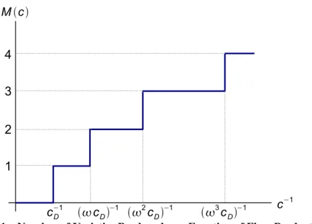
M(c) = 0 ifc > cD, max{m|c≤ωm_c D}+ 1 ifc≤cD. (8) which is (weakly) decreasing for allc∈[0, cM]. Accordingly, the number of varieties produced

by a firm with costcis indeed an integer number (and not a mass with positive measure). This number is an increasing step function of the firm’s productivity 1/c, as depicted in Figure 1 below. Firms with higher core productivity thus produce (weakly) more varieties.

Given a mass of entrantsNE, the distribution of costs across all varieties is determined by the

optimal firm product range choiceM(c)as well as the distribution of core competenciesG(c). LetMv(v)denote the measure function for varieties (the measure of varieties produced at cost

8_{Given the absence of cannibalization motive, these variety level performance measures are identical to the single}

product case studied in Melitz and Ottaviano (2008). This tractability allows us to analytically solve the closed and open equilibria with heterogenous firms (and asymmetric countries in the open economy).

9_{We will see shortly how the average price of all varieties and the number of varieties is uniquely pinned-down}

(13)

c−1 Mc cD −1 c_D−1 2c_D−1 3c_D−1 1 2 3 4

Figure 1 – Number of Varieties Produced as a Function of Firm Productivity

v or lower, givenNE entrants). Further define H(v) ≡ Mv(v)/NE as the normalized measure

of varieties per unit mass of entrants. ThenH(v) = P∞

m=0G(ωmv)and is exogenously

deter-mined fromG(.)andω. Given a unit mass of entrants, there will be a mass G(v)of varieties with cost v or less; a mass G(ωv) of first additional varieties (with cost v or less); a mass

G(ω2_v₎ _{of second additional varieties; and so forth. The measure} _H₍_v₎ _{sums over all these}

varieties.

2.3 Free Entry and Equilibrium

Prior to entry, the expected firm profit isRcD

0 Π(c)dG(c)−fE where Π(c)≡ M(c)−1 X m=0 π(v(m, c)) (9)

denotes the profit of a firm with costc. If this profit were negative for allc’s, no firms would enter the industry. As long as some firms produce, the expected profit is driven to zero by the unrestricted entry of new firms. This yields the equilibrium free entry condition:

Z cD 0 Π(c)dG(c) = Z cD 0   X {m|ω−m_c_≤_c D} π ω−mc  dG(c) (10) = ∞ X m=0 Z ωm_c D 0 π ω−mcdG(c) =fE,

where the second equality first averages over themth _{produced variety by all firms, then sums} overm.

The free entry condition (10) determines the cost cutoff cD = vD. This cutoff, in turn,

deter-mines the aggregate mass of varieties, sincevD =p(vD)must also be equal to the zero demand

price threshold in (4):

vD =

1

(14)

The aggregate mass of varieties is then M = 2γ η α−vD vD −v , (11)

where the average cost of all varieties

v = 1 M vD Z 0 vdMv(v) = 1 NEH(vD) vD Z 0 vNEdH(v) = 1 H(vD) vD Z 0 vdH(v)

depends only onvD.10 Similarly, this cutoff also uniquely pins down the average price across

all varieties: ¯ p= 1 M vD Z 0 p(v)dMv(v) = 1 H(vD) vD Z 0 p(v)dH(v).

Finally, the mass of entrants is given byNE =M/H(vD), which can in turn be used to obtain

the mass of producing firmsN =NEG(cD).

2.4 Parametrization of Technology

All the results derived so far hold for any distribution of core cost drawsG(c). However, in order to simplify some of the ensuing analysis, we use a specific parametrization for this distri-bution. In particular, we assume that core productivity draws 1/c follow a Pareto distribution with lower productivity bound1/cM and shape parameterk ≥1. This implies a distribution of

cost drawscgiven by

G(c) = c cM k , c∈[0, cM]. (12)

The shape parameterkindexes the dispersion of cost draws. Whenk = 1, the cost distribution is uniform on [0, cM]. As k increases, the relative number of high cost firms increases, and

the cost distribution is more concentrated at these higher cost levels. Askgoes to infinity, the distribution becomes degenerate atcM. Any truncation of the cost distribution from above will

retain the same distribution function and shape parameter k. The productivity distribution of surviving firms will therefore also be Pareto with shape k, and the truncated cost distribution will be given byGD(c) = (c/cD)

k

, c∈[0, cD].

When core competencies are distributed Pareto, then all produced varieties will share the same Pareto distribution: H(c) = ∞ X m=0 G(ωmc) = ΩG(c), (13) whereΩ = 1−ωk−1

> 1is an index of multi-product flexibility (which varies monotoni-cally withω). In equilibrium, this index will also be equal to the average number of products produced across all surviving firms:

M

N =

H(vD)NE

G(cD)NE

= Ω. 10_{We also use the relationship between average cost and price}_v_¯_{= 2¯}_p₋_v

(15)

The Pareto parametrization also yields a simple closed-form solution for the cost cutoffcDfrom

the free entry condition (10):

cD = γφ LΩ _k₊₂1 , (14)

whereφ ≡ 2(k+ 1)(k + 2) (cM)kfE is a technology index that combines the effects of

bet-ter distribution of cost draws (lower cM) and lower entry costs fE. We assume that cM > p

[2(k+ 1)(k+ 2)γfE]/(LΩ)in order to ensurecD < cM as was previously anticipated. We

also note that, as the customization cost for non-core varieties becomes infinitely large (ω →0), multi-product flexibilityΩgoes to 1, and (14) then boils down to the single-product case studied by Melitz and Ottaviano (2008).

2.5 Equilibrium with Multi-Product Firms

Equation (14) summarizes how technology (referenced by the distribution of cost draws and the sunk entry cost), market size, product differentiation, and multi-product flexibility affect the toughness of competition in the market equilibrium. Increases in market size, technology improvements (a fall in cM or fE), and increases in product substitutability (a rise in γ) all

lead to tougher competition in the market and thus to an equilibrium with a lower cost cutoff

cD. As multi-product flexibilityΩincreases, firms respond by introducing more products. This

additional production is skewed towards the better performing firms and also leads to tougher competition and a lowercD cutoff.

A market with tougher competition (lower cD) also features more product variety M and a

lower average price p¯(due to the combined effect of product selection towards lower cost varieties and of lower markups). Both of these contribute to higher welfare U. Given our Pareto parametrization, we can write all of these variables as simple closed form functions of the cost cutoffcD:

M = 2(k+ 1)γ η α−cD cD , p¯= 2k+ 1 2k+ 2cD, U = 1 + 1 2η(α−cD) α−k+ 1 k+ 2cD . (15)

Increases in the toughness of competition do not affect the average number of varieties pro-duced per firmM/N = Ωbecause the mass of surviving firmsN rises by the same proportion as the mass of produced varieties M.11 However, each firm responds to tougher competition by dropping its worst performing varieties (highestm) and reducing the number of varieties producedM(c).12 _{The selection of firms with respect to exit explains how the average number} of products produced per firm can remain constant: exiting firms are those with the highest cost

cwho produce the fewest number of products.

11_{This exact offsetting effect between the number of firms and the number of products is driven by our functional}

form assumptions. However, the downward shift inM(c)in response to competition (described next) holds for a much more general set of parametrizations.

12_{To be precise, the number of produced varieties}_M₍_c₎_{weakly decreases: if the change in the cutoff}_c

Dis small

enough, then some firms may still produce the same number of varieties. For other firms with high costc,M(c)

(16)

3 Competition, Product Mix, and Productivity

We now investigate the link between toughness of competition and productivity at both the firm and aggregate level. We just described how tougher competition affects the selection of both firms in a market, and of the products they produce: high cost firms exit, and firms drop their high cost products. These selection effects induce productivity improvements at both the firm and the aggregate level.13

However, our model features an important additional channel that links tougher competition to higher firm and aggregate productivity. This new channel operates through the effect of competition on a firm’s product mix. Tougher competition induces multi-product firms to skew production towards their better performing varieties (closer to their core competency). Thus, holding a multi-product firm’s product range fixed, an increase in competition leads to an in-crease in that firm’s productivity. Aggregating across firms, this product mix response also generates an aggregate productivity gain from tougher competition, over and above the effects from firm and product selection.

We have not yet defined how firm and aggregate productivity are measured. We start with the aggregation of output, revenue, and cost (employment) at the firm level. For any firmc, this is simply the sum of output, revenue, and cost over all varieties produced:

Q(c)≡ M(c)−1 X m=0 q(v(m, c)), R(c)≡ M(c)−1 X m=0 r(v(m, c)), C(c)≡ M(c)−1 X m=0 v(m, c)q(v(m, c)). (16) One measure of firm productivity is simply output per workerΦ(c) ≡ Q(c)/C(c). This pro-ductivity measure does not have a clear empirical counterpart for multi-product firms, as output units for each product are normalized so that one unit of each product generates the same utility for the consumer (this is the implicit normalization behind the product symmetry in the util-ity function). A firm’s deflated sales per workerΦR(c) ≡

R(c)/P¯/C(c) provides another productivity measure that has a clear empirical counterpart. For this productivity measure, we need to define the price deflatorP¯. We choose

¯ P ≡ RcD 0 R(c)dG(c) RcD 0 Q(c)dG(c) = k+ 1 k+ 2cD.

This is the average of all the variety pricesp(v)weighted by their output share. We could also have used the unweighted price average p¯that we previously defined, or an average weighted by a variety’s revenue share (i.e. its market share) instead of output share. In our model, all of these price averages only differ by a multiplicative constant, so the effects of competition (changes in the cutoff cD) on productivity will not depend on this choice of price averages.14

We define the aggregate counterparts to our two firm productivity measures as industry output per worker and industry deflated sales per worker:

¯ Φ≡ RcD 0 Q(c)dG(c) RcD 0 C(c)dG(c) , Φ¯R = RcD 0 R(c)dG(c) /P¯ RcD 0 C(c)dG(c) .

13_{This effect of product scope on firm productivity is emphasized by Bernard et al (forthcoming) and Eckel and}

Neary (2010).

14_{As we previously reported, the unweighted price average is} _p_¯ _{= [(2}_k_{+ 1)}_/₍₂_k_{+ 2)]}_c

D; and the average

weighted by market share is[(6k+ 2k2_{+ 3)}_/₍₂_k2_{+ 8}_k_{+ 6)]}_c

(17)

Our choice of the price deflatorP¯ then implies that these two aggregate productivity measures coincide:15 ¯ Φ = ¯ΦR = k+ 2 k 1 cD . (17)

Equation (17) summarizes the overall effect of tougher competition on aggregate productivity gains. This aggregate response of productivity combines the effects of competition on both firm productivity and inter-firm reallocations (including entry and exit). We now detail how tougher competition induces improvements in firm productivity through its impact on a firm’s product mix. In the appendix, we show that both firm productivity measures,Φ(c)andΦR(c),increase

for all multi-product firms when competition increases (cD decreases). The key component of

this proof is that, holding a firm’s product scope constant (a given number M > 1 of non-core varieties produced), firm productivity over that product scope (output or deflated sales of those M products per worker producing those products) increases whenever competition increases. This effect of competition on firm productivity, by construction, is entirely driven by the response of the firm’s product mix.

To isolate this product mix response to competition, consider two varietiesmandm0produced by a firm with costc. Assume thatm < m0so that varietymis closer to the core. The ratio of the firm’s output of the two varieties is given by

q(v(m, c)) q(v(m0_{, c}₎₎ = cD−ω−mc cD−ω−m 0 c.

As competition increases (cD decreases), this ratio increases, implying that the firm skews its

production towards its core varieties. This happens because the increased competition increases the price elasticity of demand for all products. At a constant relative pricep(v(m, c))/p(v(m0, c)), the higher price elasticity translates into higher relative demand q(v(m, c))/q(v(m0, c)) and salesr(v(m, c))/r(v(m0, c))for goodm(relative tom0).16 _{In our specific demand} parametriza-tion, there is a further increase in relative demand and sales, because markups drop more for goodmthanm0, which implies that the relative pricep(v(m, c))/p(v(m0, c))decreases.17 It is this reallocation of output towards better performing products (also mirrored by a reallocation of production labor towards those products) that generates the productivity increases within the firm. In other words, tougher competition skews the distribution of employment, output, and sales towards the better performing varieties (closer to the core), while it flattens the firm’s distribution of prices.

In the open economy version of our model that we develop in the next section, we show how firms respond to tougher competition in export markets in very similar ways by skewing their exported product mix towards their better performing products. Our empirical results confirm a strong effect of such a link between competition and product mix.

4 Open Economy

We now turn to the open economy in order to examine how market size and geography deter-mine differences in the toughness of competition across markets – and how the latter translates

15_{If we had picked one of the other price averages, the two aggregate productivity measures would differ by a}

multiplicative constant.

16_{For the result on relative sales, were are assuming that demand is elastic.} 17_Good_m_{closer to the core initially has a higher markup than good}_m0_{; see (7) .}

(18)

into differences in the exporters’ product mix. We allow for an arbitrary number of countries and asymmetric trade costs. LetJ denote the number of countries, indexed byl = 1, ..., J. The markets are segmented, although any produced variety can be exported from countrylto coun-tryhsubject to an iceberg trade cost τlh > 1. Thus, the delivered cost for varietymexported

to countryhby a firm with core competencycin countrylisτlhv(m, c) =τlhω−mc.

4.1 Equilibrium with Asymmetric Countries

Letpmax_l denote the price threshold for positive demand in marketl. Then (4) implies

pmax_l = 1

ηMl+γ

(γα+ηMlp¯l), (18)

whereMlis the total number of products selling in countryl(the total number of domestic and

exported varieties) andp¯lis their average price. Letπll(v)andπlh(v)represent the maximized

value of profits from domestic and export sales to countryhfor a variety with costv produced in countryl. (We use the subscriptll to denote domestic sales: by firms inlto destinationl.) The cost cutoffs for profitable domestic production and for profitable exports must satisfy:

vll = sup{c:πll(v)>0}=pmaxl ,

vlh = sup{c:πlh(v)>0}=

pmax_h τlh

, (19)

and thus vlh = vhh/τlh. As was the case in the closed economy, the cutoffvll, l = 1, ..., J,

summarizes all the effects of market conditions in country lrelevant for all firm performance measures. The profit functions can then be written as a function of these cutoffs:

πll(v) = Ll 4γ (vll−v) 2 , πlh(v) = Lh 4γτ 2 lh(vlh−v) 2 = Lh 4γ (vhh−τlhv) 2 . (20)

As in the closed economy,cll =vllwill be the cutoff for firm survival in country l (cutoff for

sales to domestic market l). Similarly,clh = vlh will be the firm export cutoff (no firm with

c > clh can profitably export any varieties froml toh). A firm with core competency cwill

produce all varietiesmsuch thatπll(v(m, c))≥0; it will export tohthe subset of varietiesm

such thatπlh(v(m, c))≥0. The total number of varieties produced and exported tohby a firm

with costcin countryl are thus

Mll(c) = 0 ifc > cll, max{m |c≤ωm_c ll}+ 1 ifc≤cll, Mlh(c) = 0 ifc > clh, max{m |c≤ωm_c lh}+ 1 ifc≤clh.

We can then define a firm’s total domestic and export profits by aggregating over these varieties: Πll(c) = Mll(c)−1 X m=0 πll(v(m, c)), Πlh(c) = Mlh(c)−1 X m=0 πlh(v(m, c)).

Entry is unrestricted in all countries. Firms choose a production location prior to entry and pay-ing the sunk entry cost. We assume that the entry costfE and cost distributionG(c)are common

across countries (although this can be relaxed).18 _{We maintain our Pareto parametrization (12)}

(19)

for this distribution. A prospective entrant’s expected profits will then be given by Z cll 0 Πll(c)dG(c) + X h6=l Z clh 0 Πlh(c)dG(c) = ∞ X m=0 Z ωm_c ll 0 πll ω−mc dG(c) +X h6=l ∞ X m=0 Z ωm_c lh 0 πlh ω−mc dG(c) = 1 2γ(k+ 1)(k+ 2)ck M " LlΩckll+2+ X h6=l LhΩτlh2c k+2 lh # = Ω 2γ(k+ 1)(k+ 2)ck M " Llck_ll+2+ X h6=l Lhτ_lh−kck_hh+2 # .

Setting the expected profit equal to the entry cost yields the free entry conditions:

J X h=1 ρlhLhck_hh+2 = γφ Ω l= 1, ..., J. (21)

whereρlh ≡τ_lh−k<1is a measure of ‘freeness’ of trade from countrylto countryhthat varies

inversely with the trade costsτlh. The technology indexφis the same as in the closed economy

case.

The free entry conditions (21) yield a system of J equations that can be solved for the J

equilibrium domestic cutoffs using Cramer’s rule:

chh = γφ Ω PJ l=1|Clh| |P| 1 Lh !_k₊₂1 , (22)

where|P|is the determinant of the trade freeness matrix

P ≡      1 ρ12 · · · ρ1M ρ21 1 · · · ρ2M .. . ... . .. ... ρM1 ρM2 · · · 1      ,

and|Clh|is the cofactor of itsρlh element. Cross-country differences in cutoffs now arise from

two sources: own country size (Lh) and geographical remoteness, captured by PJ

l=1|Clh|/|P|.

Central countries benefiting from a large local market have lower cutoffs, and exhibit tougher competition, than peripheral countries with a small local market.

As in the closed economy, the threshold price condition in country h (18), along with the resulting Pareto distribution of all prices for varieties sold in h (domestic prices and export prices have an identical distribution in country h) yield a zero-cutoff profit condition linking the variety cutoffvhh=chhto the mass of varieties sold in countryh :

Mh = 2 (k+ 1)γ η α−chh chh . (23)

(20)

Given a positive mass of entrants NE,l in country l, there will beG(clh)NE,l firms exporting

ΩρlhG(clh)NE,l varieties to country h.Summing over all these varieties (including those

pro-duced and sold inh) yields19

J X l=1 ρlhNE,l = Mh Ωck hh .

The latter provides a system ofJlinear equations that can be solved for the number of entrants in theJ countries using Cramer’s rule:20

NE,l = φγ Ωη(k+ 2)fE J X h=1 (α−chh) ck_hh+1 |Clh| |P| . (24)

As in the closed economy, the cutoff level completely summarizes the distribution of prices as well as all the other performance measures. Hence, the cutoff in each country also uniquely determines welfare in that country. The relationship between welfare and the cutoff is the same as in the closed economy (see (15)).

4.2 Bilateral Trade Patterns with Firm and Product Selection

We have now completely characterized the multi-country open economy equilibrium. Selection operates at many different margins: a subset of firms survive in each country, and a smaller subset of those export to any given destination. Within a firm, there is an endogenous selection of its product range (the range of product produced); those products are all sold on the firm’s domestic market, but only a subset of those products are sold in each export market. In order to keep our multi-country open economy model as tractable as possible, we have assumed a single bilateral trade costτlh that does not vary across firms or products. This simplification implies

some predictions regarding the ordering of the selection process across countries and products that is overly rigid. Sinceτlh does not vary across firms inlcontemplating exports toh, then all

those firms would face the same ranking of export market destinations based on the toughness of competition in that market,chh, and the trade cost to that marketτlh.All exporters would then

export to the country with the highestchh/τlh, and then move down the country destination list

in decreasing order of this ratio until exports to the next destination were no longer profitable. This generates a “pecking order” of export destinations for exporters from a given country l. Eaton, Kortum, and Kramarz (forthcoming) show that there is such a stable ranking of export destinations for French exporters. Needless to say, the empirical prediction for the ordered set of export destinations is not strictly adhered to by every French exporter (some export to a given destination without also exporting to all the other higher ranked destinations). Eaton, Kortum, and Kramarz formally show how some idiosyncratic noise in the bilateral trading cost can explain those departures from the dominant ranking of export destinations. They also show that the empirical regularities for the ranking of export destinations are so strong that one can easily reject the notion of independent export destination choices by firms.

Our model features a similar rigid ordering within a firm regarding the products exported across destinations. Without any variation in the bilateral trade costτlh across products, an exporter

from l would always exactly follow its domestic core competency ladder when determining the range of products exported across destinations: an exporter would never export variety

19_{Recall that}_c

hh=τlhclh.

(21)

m0 > m unless it also exported variety m to any given destination. Just as we described for the prediction of country rankings, we clearly do not expect the empirical prediction for product rankings to hold exactly for all firms. Nevertheless, a similar empirical pattern emerges highlighting a stable ranking of products for each exporter across export destinations.21 _We empirically describe the substantial extent of this ranking stability for French exporters in our next section.

Putting together all the different margins of trade, we can use our model to generate predictions for aggregate bilateral trade. An exporter in countrylwith core competencycgenerates export sales of varietymto countryhequal to (assuming that this variety is exported):

rlh(v(m, c)) = Lh 4γ v2_hh−(τlhv(m, c)) 2 . (25)

Aggregate bilateral trade fromltohis then: EXPlh =NE,lΩρlh Z clh 0 rlh(v(m, c))dG(v) = Ω 2γ(k+ 2)ck M ×NE,l ×ckhh+2Lh×ρlh. (26)

Thus, aggregate bilateral trade follows a standard gravity specification based on country fixed effects (separate fixed effects for the exporter and importer) and a bilateral term that captures the effects of all bilateral barriers/enhancers to trade.22

5 Exporters’ Product Mix Across Destinations

We previously described how, in the closed economy, firms respond to increases in competition in their market by skewing their product mix towards their core products. We also analyzed how this product mix response generated increases in firm productivity. We now show how differences in competition across export market destinations induce exporters to those markets to respond in very similar ways: when exporting to markets with tougher competition, exporters skew their product level exports towards their core products. We proceed in a similar way as we did for the closed economy by examining a given firm’s ratio of exports of two productsm0

andm, wheremis closer to the core. In anticipation of our empirical work, we write the ratio of export sales (revenue not output), but the ratio of export quantities responds to competition in identical ways. Using (25), we can write this sales ratio:

rlh(v(m, c)) rlh(v(m0, c)) = c 2 hh−(τlhω−mc) 2 c2 hh−(τlhω−m 0 c)2. (27)

Tougher competition in an export market (lowerchh) increases this ratio, which captures how

firms skew their exports toward their core varieties (recall thatm0 > mso variety mis closer

21_{Bernard et al (forthcoming) and Arkolakis and Muendler (2010) report that there is such a stable ordering of a}

firm’s product line for U.S. and Brazilian firms.

22_{This type of structural gravity specification with country fixed-effects is generated by a large set of different}

modeling frameworks. See Feenstra (2004) for further discussion of this topic. In (26), we do not further substitute out the endogenous number of entrants and cost cutoff based on (22) and (24). This would lead to just a different functional form for the country fixed effects.

(22)

to the core). The intuition behind this result is very similar to the one we described for the closed economy. Tougher competition in a market increases the price elasticity of demand for all goods exported to that market. As in the closed economy, this skews relative demand and relative export sales towards the goods closer to the core. In our empirical work, we focus on measuring this effect of tougher competition across export market destinations on a firm’s exported product mix.

We could also use (27) to make predictions regarding the impact of the bilateral trade costτlh

on a firm’s exported product mix: Higher trade costs raise the firm’s delivered cost and lead to a higher export ratio. The higher delivered cost increase the competition faced by an export-ing firm, as it then competes against domestic firms that benefit from a greater cost advantage. However, this comparative static is very sensitive to the specification for the trade cost across a firm’s product ladder. If trade barriers induce disproportionately higher trade costs on products further away from the core, then the direction of this comparative static would be reversed. Furthermore, identifying the independent effect of trade barriers on the exporters’ product mix would also require micro-level data for exporters located in many different countries (to gen-erate variation across both origin and destination of export sales). Our data ‘only’ covers the export patterns for French exporters, and does not give us this variation in origin country. For these reasons, we do not emphasize the effect of trade barriers on the product mix of exporters. In our empirical work, we will only seek to control for a potential correlation between bilateral trade barriers with respect to France and the level of competition in destination countries served by French exporters.

As was the case for the closed economy, the skewing of a firm’s product mix towards core varieties also entails increases in firm productivity. Empirically, we cannot separately measure a firm’s productivity with respect to its production for each export market. However, we can theoretically define such a productivity measure in an analogous way toΦ(c)≡Q(c)/C(c)for the closed economy. We thus define the productivity of firmcinl for its exports to destination

hasΦlh(c)≡Qlh(c)/Clh(c),whereQlh(c)are the total units of output that firmcexports toh,

andClh(c)are the total labor costs incurred by firmcto produce those units.23 In the appendix,

we show that this export market-specific productivity measure (as well as the associated mea-sureΦR,lh(c)based on deflated sales) increases with the toughness of competition in that export

market. In other words,Φlh(c)andΦR,lh(c)both increase whenchh decreases. Thus, changes

in exported product mix also have important repercussions for firm productivity.

6 Empirical Analysis

6.1 Skewness of Exported Product Mix

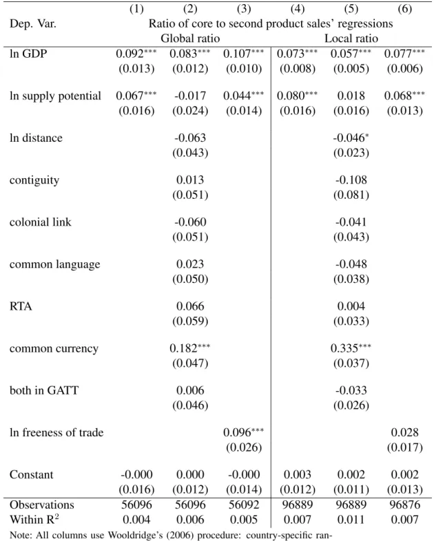
We now test the main prediction of our model regarding the impact of competition across export market destinations on a firm’s exported product mix. Our model predicts that tougher

compe-23_{In order for this productivity measure to aggregate up to overall country productivity, we incorporate the}

pro-ductivity of the transportation/trade cost sector into this propro-ductivity measure. This implies that firmcemploys the labor units that are used to produce the “melted” units of output that cover the trade cost; Those labor units are thus included inClh(c). The output of firmcis measured as valued-added, which implies that those “melted”

units are not included inQlh(c)(the latter are the number of units produced by firmcthat are consumed inh).

Separating out the productivity of the transportation sector would not affect our main comparative static with respect to toughness of competition in the export market.

(23)

tition in an export market will induce firms to lower markups on all their exported products and therefore skew their export sales towards their best performing products. We thus need data on a firm’s exports across products and destinations. We use comprehensive firm-level data on annual shipments by all French exporters to all countries in the world for a set of more than 10,000 goods. Firm-level exports are collected by French customs and include export sales for each 8-digit (combined nomenclature) product by destination country.24 _{A firm located in} the French metropolitan territory in 2003 (the year we use) must report this detailed export information so long as the following criteria are met: For within EU exports, the firm’s annual trade value exceeds 100,000 Euros;25 _{and for exports outside the EU, the exported value to a} destination exceeds 1,000 Euros or a weight of a ton. Despite these limitations, the database is nearly comprehensive. In 2003, 100,033 firms report exports across 229 destination countries (or territories) for 10,072 products. This represents data on over 2 million shipments. We re-strict our analysis to export data in manufacturing industries, mostly eliminating firms in the service and wholesale/distribution sector to ensure that firms take part in the production of the goods they export.26 This leaves us with data on over a million shipments by firms in the whole range of manufacturing sectors. We also drop observations for firms that the French national statistical institute reports as having an affiliate abroad. This avoids the issue that multinational firms may substitute exports of some of their best performing products with affiliate production in the destination country (following the export versus FDI trade-off described in Helpman et al (2004)). We therefore limit our analysis to firms that do not have this possibility, in order to reduce noise in the product export rankings.

In order to measure the skewness of a firm’s exported product mix across destinations, we first need to make some assumptions regarding the empirical measurement of a firm’s product ladder. We start with the most direct counterpart to our theoretical model, which assumes that the firm’s product ladder does not vary across destinations. For this measure, we rank all the products exported by a firm according to the value of exports to the world, and use this ranking as an indicator for the product rank m.27 We call this the firm’sglobal product rank. An alternative is to measure a firm’s product rank for each destination based on the firm’s exports sales to that destination. We call this the firm’s localproduct rank. Empirically, this local product ranking can vary across destinations. However, as we alluded to earlier, this local product ranking is remarkably stable across destinations.

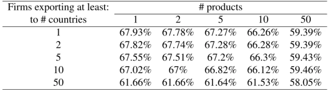
The Spearman rank correlation between a firm’s local and global rankings (in each export mar-ket destination) is .68.28 Naturally, this correlation might be partly driven by firms that export only one product to one market, for which the global rank has to be equal to the local rank. In Table 1, we therefore report the rank correlation as we gradually restrict the sample to firms that export many products to many markets. The bottom line is that this correlation remains quite stable: for firms exporting more than 50 products to more than 50 destinations, the cor-relation is still .58. Another possibility is that this corcor-relation is different across destination income levels. Restricting the sample to the top 50 or 20% richest importers hardly changes

24_{We thank the French customs administration for making this data available to researchers at CEPII.}

25_{If that threshold is not met, firms can choose to report under a simplified scheme without supplying export}

desti-nations. However, in practice, many firms under that threshold report the detailed export destination information.

26_{Some large distributors such as Carrefour account for a disproportionate number of annual shipments.}

27_{We experimented ranking products for each firm based on the number of export destinations; and obtained very}

similar results to the ranking based on global export sales.

28_{Arkolakis and Muendler (2010) also report a huge amount of stability in the local rankings across destinations.}

The Spearman rank coefficient they report is .837. Iacovone and Javorcik (2008) report a rank correlation of .76 between home and export sales of Mexican firms.

(24)

this correlation (.69 and .71 respectively).29

Table 1 – Spearman Correlations Between Global and Local Rankings Firms exporting at least: # products

to # countries 1 2 5 10 50 1 67.93% 67.78% 67.27% 66.26% 59.39% 2 67.82% 67.74% 67.28% 66.28% 59.39% 5 67.55% 67.51% 67.2% 66.3% 59.43% 10 67.02% 67% 66.82% 66.12% 59.46% 50 61.66% 61.66% 61.64% 61.53% 58.05%

Although high, this correlation still highlights substantial departures from a steady global prod-uct ladder. A natural alternative is therefore to use the local prodprod-uct rank when measuring the skewness of a firm’s exported product mix. In this interpretation, the identity of the core (or other rank number) product can change across destinations. We thus use both the firm’s global and local product rank to construct the firm’s destination-specific export sales ratio

rlh(v(m, c))/rlh(v(m0, c))form < m0.Since many firms export few products to many

destina-tions, increasing the higher product rankm0disproportionately reduces the number of available firm/destination observations. For most of our analysis, we pick m = 0 (core product) and

m0 = 1, but also report results for m0 = 2.30 Thus, we construct the ratio of a firm’s export sales to every destination for its best performing product (either globally, or in each destination) relative to its next best performing product (again, either globally, or in each destination). The local ratios can be computed so long as a firm exports at least two products to a destination (or three when m0 = 2). The global ratios can be computed so long as a firm exports its top (in terms of world exports) two products to a destination. We thus obtain these measures that are firmcand destinationhspecific, so long as those criteria are met (there is no variation in origin

l =France). We use those ratios in logs, so that they represent percentage differences in export sales. We refer to the ratios as either local or global, based on the ranking method used to compute them. Lastly, we also constrain the sample so that the two products considered belong to the same 2-digit product category (there are 97 such categories). This eliminates ratios based on products that are in completely different sectors; however, this restriction hardly impacts our reported results.

We construct a third measure that seeks to capture changes in skewness of a firm’s exported product mix over the entire range of exported products (instead of being confined to the top two or three products). We use several different skewness statistics for the distribution of firm export sales to a destination: the standard deviation of log export sales, a Herfindhal index, and a Theil index (a measure of entropy). Since these statistics are independent of the identity of the products exported to a destination, they are “local” by nature, and do not have any global ranking counterpart. These statistics can be computed for every firm-destination combination where the firm exports two or more products. The Theil and standard deviation statistics have the attractive property that they are invariant to truncation from below when the underlying distribution is Pareto; this distribution provides a very good fit for the within-firm distribution of export sales to a destination.

We graphically show the fit to the Pareto distribution in Figure 2. We plot the average share

29_{We nevertheless separately report our regression results for those restricted sample of countries based on income.} 30_{We also obtain very similar results for}_m_{= 1}_and_m0_{= 2}_.

(25)

of a firm’s export sales by product against that product’s local rank.31 _{We restrict the sample} to the top 50 products exported by firms that export between 50 and 100 products. A Pareto distribution for within-firm export sales implies a straight line on the log-log figure scale. Al-though there are clearly departures from Pareto at both ends of the distribution, the tightness of the relationship is quite striking. We also investigate the goodness of fit to the Pareto distri-bution by runningwithin firm-destination regressions of log rank on log exports (for the 7570 French firms exporting more than 10 products and less than 50 in our sample). The median R-Squared is .906, indicating a very good fit of the Pareto distribution for export sales at the firm-destination level. Thus, the truncation of export sales should not bias our dispersion mea-sured based on the Theil and standard deviation statistics.

slope = −.55, fit = .98 1 2 5 10 20 35 50 1 2 5 10 20 35 50

pct. of product in total sales of firm

rank of product in total sales of firm fitted

Figure 2 – Average share of product sales depending on the rank of the product.

6.2 Toughness of Competition Across Destinations and Bilateral Controls

Our theoretical model predicts that the toughness of competition in a destination is determined by that destination’s size, and by its geography (proximity to other big countries). We control for country size using GDP expressed in a common currency at market exchange rates. We now seek a control for the geography of a destination that does not rely on country-level data for that destination. We use thesupply potentialconcept introduced by Redding and Venables (2004) as such a control. In words, the supply potential is the aggregate predicted exports to a destination based on a bilateral trade gravity equation (in logs) with both exporter and importer fixed effects and the standard bilateral measures of trade barriers/enhancers. We construct a related measure of a destination’s foreign supply potential that does not use the importer’s fixed effect when predicting aggregate exports to that destination. By construction, foreign supply potential is thus uncorrelated with the importer’s fixed-effect. It is closely related to the construction of a country’s market potential (which seeks to capture a measure of predicted import demand for a country).32 The construction of the supply potential measures is discussed in greater detail in Redding and Venables (2004); we use the foreign supply measure for the year 2003 from Head

31_{Bernard et al (forthcoming) report a similar graph for U.S. firms exporting 10 products to Canada. They also}

find a strong goodness of fit to the Pareto distribution.

32_{Redding and Venables (2004) show that this construction for supply potential (and the similar one for market}

potential) is also consistent with its theoretical counterpart in a Dixit-Stiglitz-Krugman model. They construct those measures for a cross-section of 100 countries in 1994. Head and Mayer (2011) use the same methodology to cover more countries and a longer time period.