The Effect of Alternative Interest Rate Processes on the
Value of Mortgage-Backed Securities
Wayne R. Archer and David C. Ling*
Abstract
Analytical valuation of mortgage-backed securities (MBS) requires a process for generating future interest rates to value the embedded prepayment option. While many single-factor interest rate models are available, no systematic comparison of their effects on MBS values has been published. This article compares valuation results using three such processes—a simple log-normal process; the square-root process of Cox, Ingersoll, and Ross (CIR); and the no-arbitrage process of Black, Derman, and Toy (BDT)—selected for their prominence in the literature and their differences in major characteristics.
The study compares how well the models fit actual Treasury yield curves and their valuation of simulated MBS. The simple log-normal process is rejected for its inconsistent performance in fitting yield curves. The CIR and BDT processes value noncallable mortgagelike cash flows similarly, but the CIR process values the call option more and so has lower callable values for the MBS.
Keywords: interest rates; mortgages; prices; securitization
Introduction
The state of the art in valuing mortgage securities relies on some underlying model of risk-free (i.e., Treasury) bond yields. The traditional approach to bond pricing has been to propose a plausible model for the evolution of the short-term interest rate. This interest rate process, together with a theory of the term structure, provides a sufficient model to deduce yields (and yield volatilities) on risk-free bonds of various maturities. Once the parameters of the short-term interest rate model are chosen so that the implied yield curve (an output of the model) fits the observed yield curve on a given day as closely
as possible, claims contingent on the bond yields can be valued.1
Despite the proliferation in recent years of bond and bond-option pricing models, comparative tests have been limited. Moreover, the sensitivity of mortgage and mort-gage-backed security (MBS) values to the specification of the underlying interest rate process has not been well investigated.
This article compares values of mortgage securities on the basis of three representative models of the underlying interest rate process. It compares both security values and
*Wayne R. Archer and David C. Ling are Professors in the Department of Finance and Real Estate, College of Business Administration, University of Florida, Gainesville.
1 Examples of this approach include Courtadon (1982); Cox, Ingersoll, and Ross (1985); Dothan (1978); and
values attributed to the call (prepayment) option. The three interest rate processes are selected to represent important modeling alternatives.
Important Features of an Interest Rate Process
Mean Reversion
The interest rate processes used in valuing debt derive from equity valuation models in the tradition of Black and Scholes (1973) and Merton (1973). However, the unique attributes of debt assets have compelled adaptations. Because debt values, unlike other assets, must converge over time to par, the state variable in debt models is the interest rate rather than the asset value. However, instead of following a purely Markov or random-walk process, as assumed in the simple log-normal process of equity value models, an interest rate process, because of its underlying economics, should be mean reverting (Cox, Ingersoll, and Ross 1985; Vasicek 1977). Unlike prices of stocks and nonfinancial assets, which may reasonably follow a random walk bounded only by zero, interest rates arguably are bounded from above as well—they are increasingly likely to generate their own decline as their (real) level increases.
Specification of Conditional Volatility
Interest rate processes can vary widely in the effect of the interest rate on conditional variance. In some models, the interest rate has no effect on conditional variance (Merton 1973; Vasicek 1977). In the model of Cox, Ingersoll, and Ross (1985) (CIR), the interest rate has a proportional effect. In many other models, the interest rate has a squared effect
or greater.2 As the power of the interest rate effect increases, the heteroskedasticity of
conditional variance increases while the absolute size decreases.
It is not clear what the most appropriate specification of conditional variance is. While the proportional specification of the CIR model is derived from a general equilibrium model, giving it a strong theoretical basis, empirical tests appear to favor the higher power specifications (Chan et al. 1992).
Capacity to Replicate Observed Yield Curves
Interest rate models are typically constructed to be internally “arbitrage free” in that
“correct” prices are produced for straight discount bonds of all maturities (Koenigsberg,
Showers, and Streit 1991). This property can be ensured with “one-factor” processes in which every rate derives from movements of a single short rate. As a result, any portfolio of discount bonds or bond options is also correctly priced (i.e., of any two fairly valued portfolios, one does not outperform the other).
However, internal consistency does not ensure that an interest rate process is arbitrage free with respect to observed interest rates. In order for all debt options to be fairly priced 2 See Chan et al. (1992) for a convenient comparison of major interest rate models with respect to conditional
at a point in time, theoretical risk-free bond yields deduced from the model must exactly replicate observed Treasury yields. If not, the value of a claim based on interest rates drawn from across the term structure is likely to allow riskless arbitrage. To overcome this problem, many researchers, beginning with Ho and Lee (1986), have taken the current term structure of interest rates as an input and have developed “no-arbitrage” yield curve models that can be calibrated to exactly replicate the current yield curve.
Capacity to Replicate Market Volatilities
Accurate valuation of debt options depends not only on expected movements in interest rates (as reflected in the slope of the current yield curve), but also on the uncertainty surrounding these moves. The accurate valuation of the prepayment option embedded in fixed-rate mortgages is particularly complex because the mortgages are callable at any time before maturity. Thus, the volatilities of yields on a series of maturities all influence the value of the same call option. This series of volatilities is typically referred to as a “volatility curve.” If an interest rate model does not produce (imply) a spot volatility curve that matches that of the market (which, unlike the yield curve, cannot be observed), the model could produce inaccurate valuations of bonds and mortgages with embedded options.
Some important interest rate models are severely limited in their capacity to match the market volatility curve. Simple log-normal interest rate structures (e.g., Rendleman and Bartter 1980) produce changes proportional to the short-term interest rate that are time invariant. Also, the mean-reverting CIR model restricts the local variance to be directly proportional to the interest rate. As a result, these models imply volatility curves that may not accurately represent market expectations (Koenigsberg, Showers, and Streit 1991). To address this issue, much recent research has focused on the development of bond pricing models that both are no-arbitrage with respect to an observed yield curve and allow increased flexibility in the specification of the local interest rate volatility over time. Notable examples include the models developed by Black, Derman, and Toy (1990); Black and Karasinski (1991); Heath, Jarrow, and Morton (1990); and Hull and White (1990, 1993).
Design and Role of This Study
Despite the diverse modeling choices with regard to mean reversion, no-arbitrage, and conditional volatility, the effect of these choices on bond and mortgage pricing has not been empirically demonstrated.
The three interest rate models examined in this article reflect the major issues noted above. The first is a simple log-normal interest rate process, which is not mean reverting, has squared conditional variance, and is not no-arbitrage. The second is the CIR model, which is mean reverting but not no-arbitrage; the short rate in the CIR model has a
proportional effect on conditional variance.3 The third is a model of Black, Derman, and
Toy (1990) (BDT), which has squared variance, is mean reverting, and is no-arbitrage.
3 The CIR process is sometimes referred to as a “square-root” process because the short rate has a
Our investigation has two steps: (1) Fit each interest rate model to the actual Treasury yield curve on eight observation dates during the 1987–92 period. (2) Use the fitted interest rate processes to compare the simulated values of mortgagelike securities under a spectrum of prepayment models.
Step 1, fitting the models to the yield curve, enables us to test the models’ capacity to correctly price noncallable debt. Errors by an interest rate model in pricing noncallable cash flows create arbitrage potential. Thus, it is a necessary condition that a model price noncallable debt consistently with the yield curve. Using root mean squared error (RMSE) as a measure of goodness of fit, our first test of the models is to compare their capacity to replicate the selected actual Treasury yield curves.
Pitfalls of Published MBS Prices
It would be ideal to follow step 1 by comparing the models’ ability to price actual MBS. Unfortunately, actual prices available for this study are of doubtful quality for the purpose. Although specific MBS may be traded for immediate settlement (within five business days of the trade date), most are sold into the forward delivery market with pool information details to be provided on a “to-be-announced” (TBA) basis. This means that the securities available for delivery can vary significantly in maturity, depending on the path of interest rates for as far back as the security has been issued. A particularly troublesome result is that the degree of “burnout” (initial prepayment) in the security is only conjectured, at best. Lack of access to pool-specific data and these concerns about TBA prices compel us to use simulation tests for step 2. The three interest rate models are used to generate prices for mortgagelike instruments under three specifications of endogenous prepayment, for both near-par and discount conditions. These prepayment scenarios are selected to encompass the range of plausible prepayment activity with actual MBS.
Results
Comparing it with the BDT model, which has the property of fitting the yield curve precisely, we find that the CIR model fits the curve almost as well through a wide range of yield curves. The simple log-normal model, on the other hand, is sharply inferior in replicating the observed term structure of interest rates. The log-normal deficiency is greater the more steeply sloped and irregular the observed yield curve is. Thus, we conclude that the log-normal model is unreliable for representing interest rates. In the mortgage simulations, both the CIR and the BDT models, when calibrated with historical spot volatilities, attribute less value than the simple log-normal model to the prepayment call option embedded in the mortgages, indicating a dampening effect of mean reversion. Between the CIR and BDT models, the CIR process tends to attribute greater value to the prepayment option (and less value to the callable mortgage security), indicating a significant influence from specification of the local variance. The differences in results between the CIR and BDT models remain difficult to evaluate fully. Because, as noted above, the two models are not nested with respect to basic properties, it cannot be clearly concluded which one prices mortgagelike securities more accurately.
Special Feature of the Study
One feature of this study that bears note is that it is based on selected actual yield curve observations. In comparing alternative interest rate processes having different math-ematical structures, it is otherwise difficult to establish a basis for comparison. We believe the approach used here—fitting all models to the same actual observations— eliminates the need for conversion or interpretation in comparing parameters of different models, and no one process is given an undue normative role.
A curve-fitting approach is fundamentally different from the approach used by Chan et al. (1992) and Chen and Yang (1995), who estimate model parameters for different interest rate processes using time-series data. Since time-series estimation relies en-tirely on historical data, the resulting parameters are vulnerable to information or policy shocks. By contrast, parameters derived from fitting to a current yield curve presumably can better incorporate expectations about future interest rates.
Specifying the Interest Rate Process
Models used by the financial industry to value securities with embedded options have some common features (Koenigsberg, Showers, and Streit 1991). First, the interest rate distribution is typically based on a log-normal process, in which changes in the short-term interest rate are proportional to its level. Second, the models are constructed to be internally consistent. Third, on-the-run Treasury bonds and notes are used as bench-marks to calibrate the models to the current interest rate environment.
Simple Log-Normal
A log-normal distribution has a mean and a variance. In a simple log-normal structure, the interest rate process is specified by the observed term structure of interest rates and a single volatility—that of the short-term interest rate. This single measure of volatility is used throughout time to specify the changes in the short-term interest rate.
Define r as the instantaneous interest rate, as its expected growth rate, and as its
volatility. The simple log-normal model assumes that and are constant. This means
that r has a constant expected growth rate of – and a constant volatility of . The
process for r in a risk-neutral world is thus
dr =
(
µ σ−)
r dt+σr dz, (1)where t is time and dz is a Wiener process.
An attraction of the simple log-normal model is that, in the limit, it is geometric Brownian
motion, with a conditional variance that is proportional to the square of the interest rate.4
Empirical tests of Chan et al. (1992) indicate that models with this conditional volatility describe actual processes better than models in which conditional variance is indepen-dent of the interest rate (e.g., Vasicek 1977) or proportional to the interest rate (e.g., Cox, Ingersoll, and Ross 1985).
Rendleman and Bartter (1980) show how the continuous process described in equation (1) can be modeled using a lattice approach. The size of the up and down moves, which are
time invariant in percentage terms, along with an initial value of r, is used to generate
the lattice of all possible future values of r. The lattice is constrained to be path
independent. Prices of default-free Treasury securities are calculated by generating the cash flow (if any) in each node of the lattice and discounting backward through the lattice.
After the simple log-normal model is calibrated with assumptions for r, , and , one can
calculate the yields and the volatilities of the yields of different maturities at the initial pricing date (i.e., the spot volatility curve). The volatility curve implied by the interest rate model should match the curve that is assumed by market participants. For example, if the market uses averages of past volatilities in valuing debt instruments, the volatility curve implied by the chosen interest rate model needs to reproduce the historical volatility curve at the initial pricing date. However, the user of the simple log-normal model cannot control the volatility curve to ensure that it matches the curve assumed by the market—it is a predetermined function of the constant short-term interest rate
volatility that is used.
An important conceptual limitation of the simple log-normal model is that the volatility curve deduced from the interest rate model is relatively flat: The standard deviation of long-term yields is approximately 1 percentage point less than short rate volatilities.
This volatility curve inversion is even less pronounced for lower values of . Historically,
however, the degree of inversion in the volatility curve has been much greater than the 1-percentage-point drop produced (implied) by the simple log-normal model: On average, there has been about a 5-percentage-point drop between short- and long-term interest rate volatilities since 1985.
Another limitation of the simple log-normal model is that while changes in the shape of the yield curve over time are allowed, these changes are small. Moreover, the degree to which the simple log-normal model will allow changes in yield curve shapes is a
decreasing function of the constant that is assumed. Models that allow the local
volatility of the one-period rate to vary with time allow more diverse yield curve shapes. A final limitation of the simple log-normal model is that it lacks the property of mean reversion.
Cox, Ingersoll, and Ross
A widely recognized alternative to the simple log-normal interest rate process was offered by Cox, Ingersoll, and Ross (1985). In the equation
dr= k
(
θ−r dt)
+σ r dz, (2)is the long-term mean of r, and k is the instantaneous rate of reversion of r toward .
Thus, the first right-hand term is the short rate drift.
The CIR model has several attractive features. First, it is derived from a general equilibrium framework, which gives it theoretical appeal. Second, it embraces mean
reversion; the short rate drift is always toward . Third, the model specifies local variance
(rightmost term) as proportional to the level of interest rates. This is intuitively plausible because interest rate movements appear to be relative, and it ensures that the rate
remains nonnegative. In addition, in comparison with no-arbitrage models such as the BDT model examined below, the CIR model, with only four parameters, is much more parsimonious while still embracing properties important to the short rate process. Thus, for multiple reasons, the CIR model has become an important benchmark among interest rate processes.
Black, Derman, and Toy
The log-normal models developed by Black, Derman, and Toy (1990) and Black and Karasinski (1991) parallel the simple log-normal model in several respects: Interest rates are represented by one “factor,” the short-term interest rate. Its movement is constrained to a path-independent binomial lattice with probabilities of movement upward and
downward of p and 1 – p, respectively. Further, rate movements are logarithmic.
However, these models are more general than the simple log-normal model because the local (forward) drift and the local (forward) volatility are allowed to vary over time. This is accomplished by incorporating the current spot volatility curve into the log-normal process that describes the distribution of future interest rates.
The continuous-time limit of the BDT model may be represented as
d(ln r) = [(t) –(t)ln r]dt + (t)dz, (3)
where r is the local short-term interest rate, (t) is a time-dependent drift parameter, and
(t) depends on (t) (Hull and White 1990). That the influence of (t) is independent of
r makes this a mean-reverting process.
Three properties of the BDT model are of special interest. First, it is mean reverting. Second, like the simple log-normal model, it has the property that the local variance is proportional to the square of the interest rate. Third, the BDT model is no-arbitrage with respect to the observed yield curve.
Step 1: Estimation of Model Parameters from Observed Term Structures
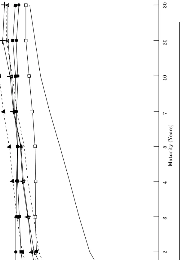
To price noncallable debt while maintaining the condition of no-arbitrage, the interest rate lattice must produce risk-free bond prices that replicate the term structure of Treasury yields and prices prevailing on the date the MBS price is observed. Otherwise, as noted above, either bonds or their derivatives will be systematically mispriced. Eight observation dates (each the last trading day in the month) were chosen over the 1987–92 period. The dates were selected to provide variation in the level and slope of the term structure, as well as expected interest rate volatility. The observed term structures ranged from slightly downward sloping (July 1989) to steeply upward sloping (January 1992), as shown in figure 1.
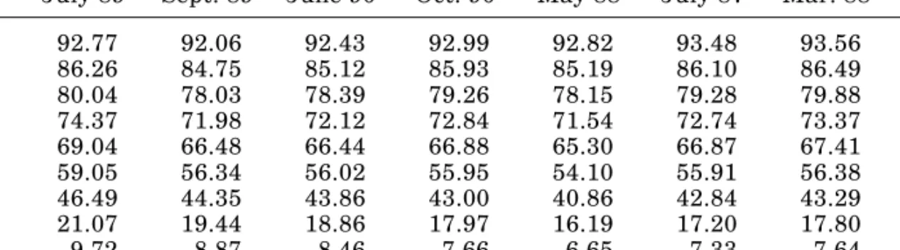
For each observation date, the three interest rate models are fitted to spot prices based on the most recently issued “on-the-run” U.S. Treasury securities with remaining maturities of 3 months, 6 months, and 1, 2, 3, 4, 5, 7, 10, 20, and 30 years. In Wall Street parlance, these on-the-run issues are securities that traded near par on the observation date. The actual prices—per $100 of face value—are reported in table 1. For example, a
10 8 6 4 2 Annual Rate (%) July 1987 May 1988 Sept. 1989 Oct. 1990 March 1988 July 1989 June 1990 Jan. 1992 Figure 1.
Observed Yield Curves (Based on Final Trading Day of Each Month)
1 2 345 7 1 0 2 0 3 0 Maturity (Years)
Table 1. Actual and BDT Discount Prices (per $100 at Face Value) Maturity
Years July 89 Sept. 89 June 90 Oct. 90 May 88 July 87 Mar. 88 Jan. 92
1 92.77 92.06 92.43 92.99 92.82 93.48 93.56 95.93 2 86.26 84.75 85.12 85.93 85.19 86.10 86.49 90.40 3 80.04 78.03 78.39 79.26 78.15 79.28 79.88 84.81 4 74.37 71.98 72.12 72.84 71.54 72.74 73.37 78.94 5 69.04 66.48 66.44 66.88 65.30 66.87 67.41 72.86 7 59.05 56.34 56.02 55.95 54.10 55.91 56.38 62.24 10 46.49 44.35 43.86 43.00 40.86 42.84 43.29 48.92 20 21.07 19.44 18.86 17.97 16.19 17.20 17.80 22.85 30 9.72 8.87 8.46 7.66 6.65 7.33 7.64 10.19
Note: Observation dates are the last trading date in each month. Spot prices are based on the most recently issued “on-the-run” U.S. Treasury securities that traded near par on the observation date. Discount prices estimated by the BDT model are, by construction, equal to the actual prices.
$100 discount Treasury bond with a remaining maturity of one year sold for $92.99 on October 31, 1990.
The remainder of this section describes the numerical procedures used to fit the three proposed interest rate process models to observed Treasury price data. Discount prices estimated by the BDT model are, by construction, equal to the actual prices, as described below.
Simple Log-Normal
The observed short-term risk-free interest rate r and estimates of and (the expected
growth rate and volatility of r) are needed to generate a lattice of risk-free bond prices and
yields for each of the observation dates. Unlike r, neither nor can be readily observed;
therefore, they must be estimated for each observation date from contemporaneous Treasury yield data. As in the empirical implementation of other option valuation
methodologies, the ’s must be exogenously specified using either implied volatilities
from market option prices or historical volatilities. For this study, we wish to maximize the comparability of data inputs among the alternative interest rate models used, and for the BDT model we must rely on historical volatility data, as explained below. Therefore, moving averages of past volatilities are employed with full recognition that they may not accurately reflect the current expectations of the marginal mortgage investor. More specifically, the annualized standard deviation of the ratio of consecutive end-of-week one-year Treasury bill rates for windows of 18 weeks is used as the (single) measure of volatility for the one-period rate.
For each of the eight observation dates, an estimate of was obtained by fitting the
simple log-normal interest rate model to spot prices. Quoted Treasury prices (adjusted for
accrued interest), r, , and p = 0.50 are exogenous inputs in the curve-fitting algorithm.
These inputs, along with a starting value for , produce the initial lattice of short-term
rates that implies a yield curve and corresponding spot prices for the various maturities.
The spot prices generated by the initial value of are then compared with the
that minimizes the (unweighted) RMSE between observed spot prices and those
produced by the lattice model.5
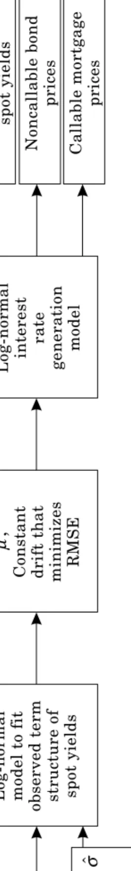
The estimation procedure for the simple log-normal model is summarized in figure 2. The
initial one-period rate r0, its estimated (constant) standard deviation , and the prices of
the benchmark Treasury securities are inputs to the model. The output is the constant
change (drift) in the one-period rate that minimizes the RMSE. The exogenously
specified r and and the estimated are then used to generate a term structure of spot
yields (prices) that in turn are used to estimate MBS prices.
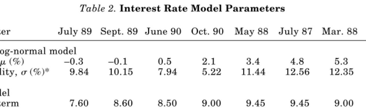
The derived ’s and the exogenous ’s for the simple log-normal model for the eight-day
sample are reported in table 2. The reported results are annualized; thus on October 31, 1990, for example, the observed yield curve was consistent with a constant annual change
in the one-period rate of 2.1 percent. The observation dates in the tables are in order
of increasing . The results indicate that the term structure over the study period was
generally upward sloping (’s averaged 2.91 percent) and that the annual standard
deviation of the short-term interest rate averaged 10.11 percent.
Table 2. Interest Rate Model Parameters
Parameter July 89 Sept. 89 June 90 Oct. 90 May 88 July 87 Mar. 88 Jan. 92 Simple log-normal model
Drift, (%) –0.3 –0.1 0.5 2.1 3.4 4.8 5.3 7.6 Volatility, (%)* 9.84 10.15 7.94 5.22 11.44 12.56 12.35 11.35 CIR model Long-term 7.60 8.60 8.50 9.00 9.45 9.45 9.00 8.30 mean of r (%) Volatility, (%) 9.84 10.15 7.94 5.22 11.44 12.56 12.35 11.35 Adjustment 1.00 0.29 0.40 0.30 0.68 0.60 0.63 0.40 speed, k
Note: Observation dates are the last trading date in each month.
*Annualized standard deviation of the ratio of consecutive end-of-week Treasury bill rates for windows of 18 weeks.
The estimated simple log-normal prices are reported in table 3 per $100 at face value. For example, the estimated price of a $100 discount Treasury security with a remaining maturity of one year is $92.88 on October 31, 1990, and the estimated price for a 30-year discount bond is $5.17; these estimated prices produced an RMSE of 1.31 percent when compared with market-derived prices. The simple log-normal RMSEs average 2.15 percent for the eight dates, and the model appears to fit flat to moderately sloped curves reasonably well. However, it is much less effective for steep yield curves, as evidenced by the higher RMSEs. Tests (not reported here) indicate that the poorer
5 Archer and Ling (1993) derive estimates of for 43 observation dates between 1987 and 1991. The average
RMSE of Treasury bond prices for these 43 dates was 0.96 percent. These RMSEs from the simple log-normal model compare favorably with the empirical results reported in other studies. For example, Brennan and Schwartz (1982) compare continuous-time model prices with actual Treasury bond prices for the 1955–79 period and report an average RMSE of 1.55 percent. Using a log-normal interest rate model similar to ours, Bhagwat, Ehrhardt, and Johnson (1991) fit month-end Treasury yield curves for 108 months from 1979 to 1987; they report an RMSE of 2.38 percent. See Giliberto and Ling (1992) for additional evidence on the simple log-normal model’s ability to replicate observed yield curves.
Figure 2.
Fitting Observed Yield Curves with the Simple Log-Normal Model
Log-normal model to fit observed term structure of spot yields
Term structure of spot yields Noncallable bond prices Callable mortgage prices Log-normal interest rate generation model
Constant drift that minimizes RMSE
ˆ,µ Note: r0
= initial one-month rate;
ˆ
σ
= expected (constant) volatility of one-month rate;
ˆ
µ
= constant drift in
r
that best fits observed term structure data
on given day.
ˆσ r0
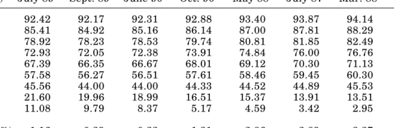
Table 3. Simple Log-Normal Discount Prices (per $100 at Face Value) Maturity
(Years) July 89 Sept. 89 June 90 Oct. 90 May 88 July 87 Mar. 88 Jan. 92
1 92.42 92.17 92.31 92.88 93.40 93.87 94.14 96.01 2 85.41 84.92 85.16 86.14 87.00 87.81 88.29 91.85 3 78.92 78.23 78.53 79.74 80.81 81.85 82.49 87.55 4 72.93 72.05 72.38 73.91 74.84 76.00 76.76 83.11 5 67.39 66.35 66.67 68.01 69.12 70.30 71.13 78.56 7 57.58 56.27 56.51 57.61 58.46 59.45 60.30 69.21 10 45.56 44.00 44.00 44.33 44.52 44.89 45.53 55.00 20 21.60 19.96 18.99 16.51 15.37 13.91 13.51 16.75 30 11.08 9.79 8.37 5.17 4.59 3.42 2.95 2.59 RMSE (%) 1.16 0.39 0.22 1.31 2.86 2.89 3.27 5.16
Note: Observation dates are the last trading date in each month.
performance with steep yield curves is partly attributable to the inability of a single drift parameter to fit multiple slopes, which are often associated with a steep yield curve.
Cox, Ingersoll, and Ross
While numerous studies have estimated a CIR interest rate process in some context (e.g., Brown and Dybvig 1986; Buser, Hendershott, and Sanders 1990; Chan et al. 1992), none appears to have fitted the model to a specific observed term structure, as required in this
study. The approach used here is to estimate (volatility) externally as described above
and then use a numerical search over values of k (speed of adjustment) and (long-term
mean of r).
Though the CIR process usually has been used as a continuous-time model, it also can be represented in discrete lattice form. Nelson and Ramaswamy (1990) have derived a binomial lattice version that converges in probability distribution to the continuous CIR process. Since the initial CIR lattice is path dependent—or, in their terms, “not computationally simple”—they find a transform from the binomial CIR lattice to a lattice that is computationally simple. The inverse of this transform can then be used to generate CIR values from the simple lattice. The Nelson-Ramaswamy model, with corrections as offered by Tian (1993), is used here to represent the CIR model.
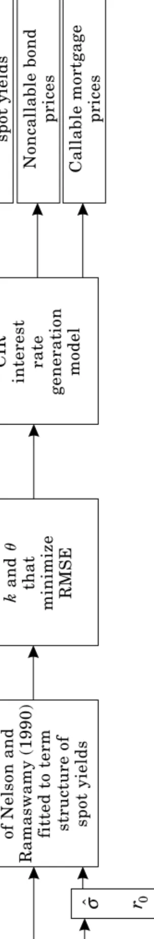
The estimation procedure for the CIR model is summarized in figure 3. The initial
one-period rate r0, its estimated standard deviation , and the prices of the benchmark
Treasury securities are inputs to the model. The procedure searches for the pair of values
and k from equation (2) that minimizes the RMSE in estimating reference spot prices
of the observed yield curve. Because this procedure has not been proved to minimize
RMSE, care was taken to examine the “surface” of RMSEs in – k space for the risk of
obtaining a strictly local minimum. No evidence of such risk was detected, as the surface was smooth and well behaved for the regions examined. As a final step in the procedure,
the exogenously specified r and and the estimated and k are used to generate a term
Term structure of spot yields Noncallable bond prices Callable mortgage prices CIR interest rate generation model Note: r0
= initial one-month rate;
ˆ
σ = expected volatility of one-month rate;
= long-term mean of r ; k = rate of reversion of r toward . Figure 3.
Fitting Observed Yield Curves with the CIR Model
Lattice CIR model
of Nelson and
Ramaswamy (1990)
fitted to term structure of spot yields
k and that minimize RMSE ˆσ r0
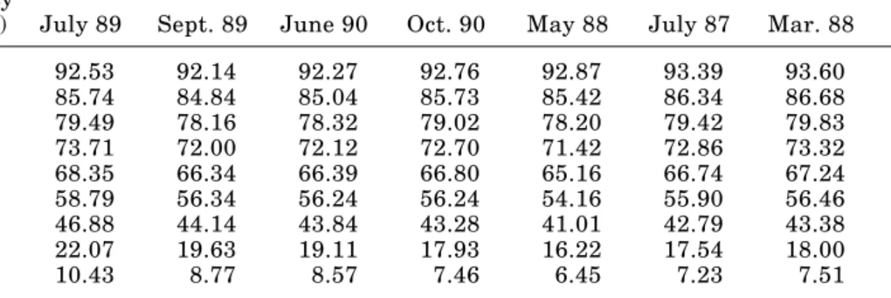
The results of the curve-fitting process for the CIR model are reported in table 4. The average RMSE over the eight observation dates is 0.23 percent, less than a ninth of that for the simple log-normal model. In contrast to the simple log-normal case, RMSEs for the CIR model do not correlate with the slope of the yield curve.
Table 4. CIR Discount Prices (per $100 at Face Value) Maturity
(Years) July 89 Sept. 89 June 90 Oct. 90 May 88 July 87 Mar. 88 Jan. 92
1 92.53 92.14 92.27 92.76 92.87 93.39 93.60 95.47 2 85.74 84.84 85.04 85.73 85.42 86.34 86.68 90.08 3 79.49 78.16 78.32 79.02 78.20 79.42 79.83 84.34 4 73.71 72.00 72.12 72.70 71.42 72.86 73.32 78.59 5 68.35 66.34 66.39 66.80 65.16 66.74 67.24 72.99 7 58.79 56.34 56.24 56.24 54.16 55.90 56.46 62.62 10 46.88 44.14 43.84 43.28 41.01 42.79 43.38 49.47 20 22.07 19.63 19.11 17.93 16.22 17.54 18.00 22.34 30 10.43 8.77 8.57 7.46 6.45 7.23 7.51 10.12 RMSE (%) 0.60 0.12 0.13 0.20 0.13 0.17 0.13 0.39
Note: Observation dates are the last trading date in each month.
Black, Derman, and Toy
In contrast to the three parameters of the simple log-normal model and the four parameters of the CIR model, the BDT model requires a volatility parameter and a rate
parameter for each period: 360 pairs for the maturity of a standard 30-year monthly
mortgage.
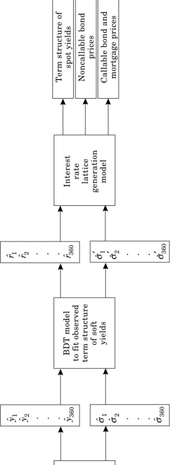
The two-step procedure summarized in figure 4 was used to implement the BDT model. The first step was to fit complete monthly yield and volatility curves. Of the 360 monthly yields that are required as inputs to the BDT model for each observation date, 11 are contained in our data set from benchmark Treasury securities (3 months, 6 months, and 1, 2, 3, 4, 5, 7, 10, 20, and 30 years). The remaining 349 spot yields are estimated by interpolation. For the volatilities, we estimated an 18-month moving average of monthly yield changes from January 1987 through April 1992 on constant-maturity treasuries, as
reported in the Federal Reserve Bulletin, to obtain the 11 spot volatilities that correspond
to the benchmark securities. The remaining 349 spot volatilities are fitted from these 11. The second step was to transform the spot yield curve and the spot volatility curve into a schedule of local volatilities and a schedule of maximum forward rates for the BDT lattice. The local volatilities were derived from the spot volatility curve using the fact that each spot volatility is a geometric average of the embedded local volatilities.
We found the schedule of maximum forward rates by a procedure that followed examples by Black, Derman, and Toy (1990). Sequentially, from the beginning of the lattice, for each period we constructed a test array of forward rates such that the local volatility was constant throughout the array and consistent with the previously derived schedule of local volatilities. We then used the lattice generated up through that period to derive an implied spot price and hence the implied spot rate. We shifted the test array (vertical
Yield curve data on benchmark Treasury securities
Term structure of
spot yields
Noncallable bond
prices
Callable bond and mortgage prices
Interest rate lattice
generation
model
Figure 4.
Fitting Observed Yield Curves with the BDT Model BDT model to fit observed term structure of soft yields ˆy1 ˆy2 . . . ˆy360 ˆr1 ˆr2 . . . ˆr360
Maximum rates Local volatilities
ˆσ1 ˆσ2 . . . ˆσ360 ˆ ˆ . . . ˆ ′ ′ ′ σ1 σ2 σ360 Note: ˆy1 , . . . , ˆy360
= estimated spot yields;
ˆσ1
, . . . ,
ˆσ360
estimated spot volatilities;
ˆr, . . . ,1 ˆr360
= maximum one-month forward rates;
ˆ ′, . . . ,σ1 ˆ ′ σ360 , = local
vector) of forward rates until the implied spot rate obtained from the process matched the spot yield curve. The lattice derived in this manner is fully preserved in the two output arrays—the schedule of local volatilities and the schedule of maximum forward rates. Using the numerical procedure described above, the BDT interest rate model was fitted to the eight observed yield curves (table 1). Note that the RMSEs are 0 because BDT prices for the benchmark securities are equal to the actual market prices, by construction.
Comparing Goodness of Fit
With a flat yield curve, both simple log-normal and CIR models compare favorably with observed prices. For example, while most generated prices for September 1989 lie above the actual prices, the divergence generally is small. The only exception is the 30-year price for the simple log-normal model, which is noticeably higher than the actual price. A much more drastic divergence occurs with steep yield curves. While the CIR model still matches the actual curve very closely, the simple log-normal model diverges sharply. For example, through 10 years, the simple log-normal prices for July 1987 lie noticeably above the actual prices, but after 10 years they lie even more sharply below. This is consistent with the finding that the RMSE for the simple log-normal model increases significantly as the actual yield curve steepens.
The problem with the simple log-normal model seems to be that the actual yield curve is steeper in the first year than it is later. The model, with a single drift parameter, must compromise between the slopes of the two regions of the curve. This compromise is very sensitive to the inflection of the yield curve.
Dispersion of Short-Term Interest Rates
By invoking the local expectations hypothesis, the entire term structure of interest rates at any node in the lattice can be determined solely from subsequent movements in the one-period rate. The longer the maturity of an interest rate option, the more time there is for the one-period rate, and therefore the rates on all maturities, to change from the original level. Thus, an increased dispersion of interest rates increases the probability that a call option will be exercised.
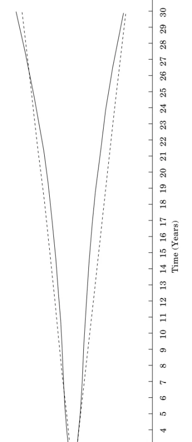
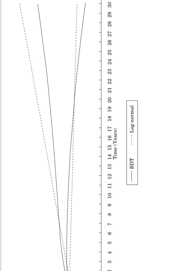
With a log-normal distribution, changes in the one-period interest rate are proportional to the level. Thus, over longer time intervals, the dispersion of the one-period rate grows faster and is asymmetric in absolute terms. Historically, however, interest rates have tended to exhibit a pattern of mean reversion. This theoretical weakness of the simple log-normal model is overcome with the explicitly mean-reverting CIR process. Because the BDT model allows the local interest rate process to change over time, the degree of dispersion assumed by the model can be made consistent with historical volatilities. To examine the relative degree of interest rate dispersion, the outer branches of the interest rate lattice implied by the simple log-normal and BDT models are plotted for each of the eight sample dates. The results for September 1989, which are representative of
flat term structure environments, are illustrated in figure 5. Those for January 1992, which are representative of steeply sloped term structures, are illustrated in figure 6. As the time from the pricing date increases, the rate envelopes for both models widen. But extreme interest rates, especially with steeply sloped term structures, are less likely with the BDT model than with the simple log-normal model because the BDT model is mean reverting. Note that, because of the asymmetric effects of relative rate changes, the reduction in extreme BDT rates—relative to the simple log-normal model—is more pronounced for interest rate increases than for decreases. This reduction in the overall level of interest rates will unambiguously increase the relative value of BDT cash flows. In addition, less variation in the one-period rate (and therefore in longer term rates) will result in fewer states of the world in which it is optimal for the borrower to exercise the call option. Both the increase in the value of the noncallable cash flows and the reduced value of the call option should imply higher MBS values using the BDT model instead of the simple log-normal model, all else being equal.
Although not shown in figures 5 and 6, the rate envelope of the CIR interest rate lattice would fall between those of the simple log-normal and BDT models. The CIR interval is narrower than that for the simple log-normal model because the CIR model has mean reversion. The CIR interval is wider than the BDT interval because the CIR model has a higher conditional interest rate volatility.
Conclusions
Using RMSE as a measure of goodness of fit, we can draw definite conclusions about the ability of the CIR and simple log-normal models to price noncallable debt cash flows. In all except the simplest cases of flat yield curves, the CIR model dominates the simple log-normal model. Average RMSE for the simple log-log-normal model is more than nine times that for the CIR model. This confirms, as expected, that the simple log-normal model generally is inferior as a model of interest rate processes. Of special interest is the curve-fitting ability of the CIR model.
Step 2: A Model for the Valuation of Mortgage-Backed Securities
State-of-the-art MBS valuation models are based on the neoclassical model of perfect competition; that is, the mortgage market is assumed to be fully integrated with the general capital market. Thus, mortgage and MBS rates in the perfect markets model are determined by the yield on long-term noncallable Treasury bonds and the values of the embedded call and default options.
The bulk of MBS research has abstracted from explicit modeling of the house price process and default risk and has focused on the borrower’s option to call the mortgage at par. One justification for this approach is that MBS investors are typically fully insured against loss of capital, so defaults look like prepayments to them. In the model developed below, the probability of default is incorporated into the exogenously specified
probabil-Figure 5.
BDT versus Log-Normal Interest Rate Envelope, Flat Yield Curve (September 1989)
BDT Log-normal Short Rate (%) 1,000 100 10 1 0 Note:
The curves trace the outer branches of the short-term interest rate lattice. The rate envelope of the CIR lattice falls betwee
n those for the simple
log-normal and BDT models.
1 2 3 4 5 6 7 8 9 1 01 1 1 21 31 4 1 5 1 6 1 7 1 8 1 9 2 02 1 2 22 32 4 2 52 6 2 72 8 2 93 0 Time (Years)
Figure 6.
BDT versus Log-Normal Interest Rate Envelope, Steep Yield Curve (January 1992)
1 2 3 4 5 6 7 8 9 1 01 1 1 21 31 4 1 5 1 6 1 7 1 8 1 9 2 02 1 2 22 32 4 2 52 6 2 72 8 2 93 0 Time (Years) BDT Log-normal 10,000 1,000 100 10 1 0 Short Rate (%) Note:
The curves trace the outer branches of the short-term interest rate lattice. The rate envelope of the CIR lattice falls betwee
n those for the simple
ity that a non-interest-rate-driven prepayment will occur. This approach to modeling
default is justified if the prepayment and default decisions are uncorrelated.6
With respect to interest-rate-driven prepayments, it is widely recognized that the mortgage borrowers use the call option less ruthlessly than frictionless optimal call models imply. Many borrowers fail to exercise well-into-the-money options, while others prepay when the call option is out of the money. The existence of this “suboptimal” prepayment behavior has forced academics and practitioners to seek alternatives to the optimal (fully endogenous) call model of mortgage prepayment. The typical response of both academics and practitioners has been to displace the optimal call model with more adaptable, fully exogenous treatments of prepayment (e.g., Schwartz and Torous 1989, 1992). Archer and Ling (1993) develop a rational model of mortgage prepayment that incorporates both types of nonoptimal prepayment and retains endogenous call. In addition, by recognizing heterogeneous borrower transaction costs, the model presents a way to account more precisely for the varying prepayment lags associated with well-into-the-money call options.
Principal Assumptions
To implement the MBS valuation procedure, we follow Archer and Ling (1993) and assume the following:
1. Time is divided into discrete periods of equal length. There are 12 periods or
intervals per year. All cash flows occur at these discrete points.
2. The one-period risk-free interest rate, the source of all uncertainty in the model, is
a random variable following a discrete jump process.
3. In each state of the world, there is an exogenously specified probability that a
non-interest-rate-driven prepayment will occur.
4. Conditional on not prepaying for exogenous reasons, mortgage borrowers act to
maximize wealth by adopting prepayment strategies that maximize any gains that result from a decline in mortgage interest rates to a level below the contract interest rate.
5. Exercise of the call option is impeded by transaction costs, and borrowers are
heterogeneous in the transaction costs they face.
6. There are no taxes and no extra costs for borrowing.
Assumption 1 implies that borrower decisions about continuing the current mortgage or terminating it through prepayment take place at the instant before the payment is to be remitted. The discrete jump processes for the one-period interest rate that we model are
6 Kau et al. (1992) and others have pointed out that the probabilities of default and
interest-rate-driven prepayments are at least partly correlated. Thus, in theory, both probabilities must be determined simultaneously.
the three models detailed above. The exogenously specified probability that a prepay-ment will occur (assumption 3) is meant to capture general equilibrium wealth-maximi-zation decisions that are too complex to be reflected in a partial equilibrium or application-based pricing model. By incorporating heterogeneous transaction costs (assumption 5), the model offers a way to account for the varying degrees of nonresponsiveness that borrowers display toward in-the-money call options.
Notation
It is assumed that all loans in the MBS pool carry identical contract terms and amounts and were originated at date 0. The value of a mortgage in the pool differs according to the level of transaction costs faced by the borrower. The initial pool of borrowers is stratified
into n types, each of which has a discrete level of transaction costs. Borrowers within each
type are assumed to behave identically with respect to changes in interest rates. The value of the MBS at any point in time is the sum of the mortgage values held by borrowers in the transaction cost types that have not prepaid.
To formalize the model, the following notation is introduced:
L0 = original mortgage loan amount
m0 = fixed periodic mortgage rate for a loan originated at date 0
P0 = monthly mortgage payment on a loan originated at date 0 at rate m0
Lt(L0, m0) = unpaid principal balance at date t on a loan originated at date 0 after
the scheduled payment is made
t = probability of terminating the mortgage at date t for non-interest-rate
reasons, conditional on the borrower’s not having previously termi-nated
it = prepayment or refinancing costs expected to be incurred by borrower
type i at time t
Bit(r; t, m0, ) = value to borrower type i at date t of a callable mortgage liability
originated at date 0 < t, where r = Rt( j) is the one-period spot interest
rate observed at date t in state j, m0 is the (original) contract rate, and
is a vector of parameters governing the underlying interest rate
process
Vit(r; t, m0, ) = value to the MBS investor at date t of a callable mortgage of type i
originated at date 0
Note that, by assumption, only Bit(r; t, m0,) and Vit(r; t, m0,) are state dependent—
that is, dependent on the realization of the one-period spot interest rate r. The subscript
j, which denotes the vertical position in the interest rate or valuation trees at time t, is
Recursive Solution
The ith borrower type prepays for nonfinancial reasons with probability t at each date
t. This exogenous prepayment probability may vary with time but is assumed to be
independent of the interest rate process. Conditional on the absence of nonfinancial
termination at date t, the borrower has two choices to consider: (1) exercise the
prepayment call option or (2) continue the mortgage as is for an additional period. The existence of nonzero transaction costs effectively raises the exercise price of the call option. Once the costs of the two alternatives are determined, the (absolute) value of the
borrower’s mortgage liability, Bit(r; t, m0, ), is defined by the cost of non-interest-rate
termination (occurring with probability t) and the minimum-cost financial strategy
(occurring with probability 1 – t).
Investors in mortgage pass-through securities receive their prorated share of periodic payments (both principal and interest) on the underlying mortgages, minus servicing
costs retained by the MBS servicer. Define as the fraction of the mortgage balance that
is paid to the servicer. The investor receives the scheduled payment net of these servicing costs, plus the remaining mortgage balance if exogenous prepayment occurs or if, conditional on nontermination, calling is the borrower’s least cost strategy. If prepaying the mortgage is the borrower’s least cost strategy, then the MBS investor receives the scheduled payment plus the remaining loan balance, net of the servicing costs. Thus,
Vit(r; t, m0, ) = P0 + (1 – )Lt(L0, m0) if the borrower prepays.
Let Cit(r; t, m0, ) be the value of the ith mortgage type to the investor, excluding the
current payment, if exogenous prepayment does not occur and the borrower chooses the
continuation strategy. The value of the ith mortgage type at date t is therefore
V r m P L L m P L L m P L L m C r m it t t t t t t it t ; , , , , , ; , , ρ α ρ α ρ α ρ 0 0 0 0 0 0 0 0 0 0 0 1 1 1
(
)
= +(
−)
(
)
+(
−)
(
)
[
]
+(
−)
[
−(
)
+(
)
]
if borrower calls, or if borrower continues. (4)Note that the value of the ith mortgage type to the investor in any node, Cit(r; t, m0, ),
is less than the value (cost) of the mortgage liability to the borrower, because the borrower incurs third-party servicing costs that are not received by the MBS investor.
The solution procedure is recursive: Bit+1(r; t, m0, ), along with the values at date t of
the other variables and parameters, is used to determine Bit(r; t, m0, ). Optimal
borrower strategies and the rate of exogenous prepayment, in turn, determine the cash
flows and the value of the ith mortgage type to the investor. The procedure moves
backward one period (month) in time until the current value of the ith mortgage type is
established. Because of third-party transaction costs and servicing costs, separate lattices for the borrower and investor valuations must be constructed. Keeping track of
Bit(r; t, m0,) separately from Vit(r; t, m0,) captures the wedge, or asymmetry, between
borrowers’ and investors’ valuations of the underlying mortgages. This valuation
Quantifying the Effect of the Assumed Interest Rate Distribution on MBS Prices
Simulated call option values and prices of mortgagelike securities for the eight observa-tion days are presented in this secobserva-tion. The primary purpose is to quantify the importance of the underlying model of interest rates in determining prices of these securities.
Spectrum of Prepayment Models Used
Mortgage prepayment behavior cannot be explained by “pure” interest rate options alone, and much research remains to be done to understand the other factors involved. To account for the limited understanding of prepayment, a range of prepayment models and mortgage coupon scenarios is considered. At one end of the spectrum, we specify a pure driven prepayment model without transaction costs. As a second, less pure option-driven model, we superimpose a constant probability of exogenous prepayment over the model, as discussed below. Still less option-sensitive is a prepayment model that incorporates both exogenous prepayment and a distribution of transaction costs. Finally, in addition to examining callable prices of near-par mortgagelike securities, we examine discount securities for which the influence of the call option would be expected to be minimal. To the extent that results of our comparisons are invariant across this range of models and scenarios, we can gain confidence that conclusions are independent of the prepayment specification.
Assumptions
An exogenous prepayment parameter, t, is set at either 0 or 4 percent. The 4 percent
derives from studies by Richard and Roll (1989) of prepayment rates for Government National Mortgage Association (GNMA) pools from 1979 to 1988. For deeply discounted pools (mortgage rates at least 200 basis points below market), Richard and Roll report annual prepayment rates ranging from 2.3 to 4.7 percent, with most near 4 percent. Because borrower call options on the underlying mortgages are far out of the money for these deeply discounted mortgage pools, their historical prepayment rates are assumed to reflect only non-interest-rate factors such as relocation, household dissolution, and economic distress. In particular, these prepayment rates include borrower defaults because MBS are fully insured; thus, all terminations look like prepayments to the MBS investor.
To empirically determine an appropriate distribution of transaction costs, the MBS valuation model was fitted to actual yield curves and GNMA price data using the simple log-normal model of interest rates. Our data sample is end-of-month closing prices from July 1987 through January 1991. This interval was selected because it contained a fairly representative range of interest rate environments for the previous 8 to 10 years. By assuming that the distribution of transaction costs is log-normal and that only 1 percent of the distribution is smaller than 4 percent of the mortgage balance, we
inferred a distribution of transaction costs from the price variation of the GNMA sample.7 The arithmetic mean of the fitted distribution is approximately 32 percent. This result seems roughly consistent with the evidence of Stanton (1992), who reports that transac-tion costs may range upward to 40 percent. On the basis of these empirical findings, we assume log-normally distributed transaction costs with a mean of 32 percent for the mortgage simulations that follow.
The intervals of transaction costs are selected so that each has an equal cumulative probability. In the experiments reported below, 10 intervals are used, each representing 10 percent cumulative probability of a log-normal distribution. For each interval, the value of transaction costs assigned is the (approximate) conditional expected value for the range. Precision in assigning the expected value of the transaction costs for each interval is a second-order concern, since the tails of the distribution are truncated, resulting in a nonnormal distribution in any case. The distribution is bounded below by some level of transaction costs greater than zero and bounded above by the minimum level of transaction costs that prevents exercise of the call option.
Mortgage Pricing Results
Three properties of interest rate processes are the focus of this study: mean reversion, influence of the short-term interest rate on local volatility, and the property of no-arbitrage. The three interest rate processes examined have various combinations of these features, as summarized in table 5. The results of step 1 in this investigation lead us to reject the simple log-normal model (without mean reversion) as inadequate in many cases to represent an interest rate process; it fails to meet the necessary condition of replicating the yield curve. Thus we focus primarily on the two mean-reverting processes: the CIR model, with proportional local variance but without the property of no-arbitrage, and the BDT model, with squared variance and the property of no-arbitrage. With two features and only two models, it is not possible to isolate the effects of each feature without further restrictions. Thus it is important to note that the findings in step 1 of the investigation reveal an additional empirical restriction. The RMSEs, reported in tables 3 and 4, reveal no significant gain from using the no-arbitrage interest rate model to fit the yield curve. That is, this study finds no substantial difference between the CIR and BDT models in the value placed on (noncallable) cash flows. This result is useful, since the no-arbitrage feature, by definition, should have its primary influence here rather than on the value of options.
The minimal influence of the no-arbitrage characteristic reduces the dimensionality of the models to one characteristic—specification of the local variance—and enables us to isolate its effect. By this reasoning, any systematic difference in values resulting from the CIR and BDT models is attributable to the difference between the squared and propor-tional effects of rate on variance.
Simulations of MBS Values
Results of the numerical experiments are presented in table 6. The eight observation dates are arranged in order of increasing yield curve slope. Each underlying mortgage is 7 For details of this fitting process, see Archer and Ling (1993).
Table 5. Comparative Features of Three Interest Rate Processes Effect of Short
Rate on
Process Mean Reversion Conditional Volatility No-Arbitrage
Simple log-normal No Squared No
CIR Yes Proportional No
BDT Yes Squared Yes
assumed to be newly originated, with a term of 30 years, with monthly payments and no prepayment penalty. The first step in the numerical procedure was to determine the coupon rate for each observation date that would price a noncallable MBS security at par
equal to $100.8 Price differences between the BDT and CIR models are reported in the
table. Using the estimated noncallable coupon rate, both noncallable prices and callable prices were then estimated for each of the models under three sets of assumptions: (1) no
prepayment costs and no exogenous prepayment (t = 0); (2) no prepayment costs and
exogenous prepayment (t = 0.04); (3) 24 percent average prepayment costs and
exog-enous prepayment (t = 0.04). Parallel estimates were completed for discount mortgages
(coupon rate 150 basis points below the near-par coupon), and the results appear in the lower half of table 6.
The three panels of table 6 can be regarded as a spectrum of prepayment specifications. From left to right they present (1) the maximum option value, an unmitigated ruthless option specification; (2) mitigation of the option by exogenous prepayment only; and (3) mitigation of the option by both exogenous prepayment and a distribution of transaction costs. The near-par cases in the upper three panels represent a high potential prepay-ment incentive (large option values), while the discount cases should represent a significantly lower potential. The smaller option value for the discount coupons might derive not only from the below-market coupon on the mortgages but also from lagged exercise behavior or other mitigants of prepayment. Thus, while true prepayment behavior cannot be identified, the results of table 6 should bound the true behavior; any systematic findings should apply to the true prepayment behavior.
Effect of Squared versus Proportional Influence of Rate on Local Variance The results in table 6 are presented in terms of the option value equation (callable value equals noncallable value less option value). The “callable value difference” is equal to the fully callable BDT price minus the fully callable CIR price. This total value difference is broken down into its component parts: the difference in the noncallable prices and the
difference in the call option values. For example, with t = 0.00 (leftmost panel) and the
July 1989 term structure environment, the BDT MBS price was $0.44 (or 44 basis points) greater than the CIR price. This 44-basis-point difference has two components: First, the BDT interest rate lattice placed a $1.07 lower value on the noncallable cash flows. Second, the BDT model attributes $1.51 less value to the interest rate call option than the CIR model does.
8 Near-par coupons are determined by use of the simple log-normal interest rate model. While subsequent
investigation revealed the limitations of this model, its use here to approximate a near-par coupon poses no substantive problems for the research.
Table 6.
Price Difference, BDT – CIR (per $100 of Par Value)
No Exogenous Prepayment 4% Exogenous Prepayment 4% Exogenous Prepayment ( t = 0.00), ( t = 0.04), ( t = 0.04), No Prepayment Costs No Prepayment Costs
Average 24% Prepayment Costs
MBS Callable Noncallable Option Callable Noncallable Option Callable Noncallable Option Coupon Value Value Value Value Value Value Value Value Value Date Rate (%)* Difference Difference Difference Difference Difference Difference Difference Difference Difference
Near par July 89
7.74 0.44 – 1.07 – 1.51 0.78 – 0.45 – 1.23 – 0.41 – 0.45 – 0.04 Sept. 89 8.13 3.85 0.02 – 3.83 3.38 0.02 – 3.37 1.23 0.02 – 1.22 June 90 8.27 1.87 – 0.12 – 1.99 1.80 – 0.27 – 2.07 0.20 – 0.27 – 0.47 Oct. 90 8.59 1.20 0.15 – 1.05 0.88 0.06 – 0.82 0.20 0.06 – 0.14 May 88 8.68 – 0.22 0.14 0.36 0.21 0.05 – 0.16 – 0.02 0.05 0.07 July 87 8.82 0.78 – 0.06 – 0.85 0.81 – 0.04 – 0.84 – 0.03 – 0.04 – 0.01 March 88 8.79 0.61 0.01 – 0.60 0.42 0.00 – 0.42 0.15 0.00 – 0.15 Jan. 92 7.45 0.74 0.49 – 0.25 0.29 0.30 0.01 0.65 0.30 – 0.35 Discount July 89 6.24 – 0.92 – 0.92 0.00 – 0.39 – 0.39 0.00 – 0.38 – 0.39 – 0.01 Sept. 89 6.63 0.47 0.02 – 0.45 0.51 0.02 – 0.50 0.04 0.02 – 0.03 June 90 6.77 – 0.07 – 0.10 – 0.04 – 0.05 – 0.08 – 0.03 – 0.08 – 0.08 0.01 Oct. 90 7.09 0.13 0.13 0.00 0.06 0.05 – 0.01 0.05 0.05 0.00 May 88 7.18 0.08 0.12 0.04 0.02 0.04 0.02 0.04 0.04 0.00 July 87 7.32 – 0.22 – 0.05 0.16 – 0.13 – 0.03 0.10 – 0.04 – 0.03 0.01 March 88 7.29 – 0.09 0.01 0.10 – 0.06 0.00 0.06 0.00 0.00 0.00 Jan. 92 5.95 0.47 0.42 – 0.05 0.29 0.26 – 0.03 0.26 0.26 0.00 Note:
Callable value difference is equal to noncallable value difference minus option value difference.
*Each underlying mortgage is newly originated with a term of 30 years and monthly payments. The MBS coupon rate for each observ
ation date is the rate
that prices a noncallable MBS at par ($100). Coupon rates on discount securities are 150 basis points below those for the
Except for the most negatively sloped and most positively sloped yield curves (first and last rows in each panel), the BDT and CIR models value noncallable cash flows essentially the same. This is consistent with the finding in table 4 of close CIR fits to the yield curve in all but the two extreme-slope cases.
By contrast to the similarity of noncallable values, the CIR model tends to produce larger option values than the BDT model—37 out of 48 option value differences either are zero or are larger for the CIR model, and the exceptions tend to be small. Since both models have mean reversion, this difference suggests that the difference in volatility specifica-tion is significant. The interest rate in the CIR model affects condispecifica-tional (local) variance proportionally rather than by a squared effect. This means that at a given interest rate, the conditional volatility of the CIR model must be larger than for the BDT model, since the interest rate is less than one, and its value diminishes as its exponent increases. That is, the CIR model tends to have a wider dispersion of rates than the BDT model, implying higher value for the prepayment option.
Effect of Mean Reversion
Despite the conclusion from the first part of this study that the simple log-normal model is inadequate as an interest rate process, the model is of interest for its combined properties of squared volatility and lack of mean reversion. Selective comparisons of results from the simple log-normal process with those from the CIR process give an indication of the importance of mean reversion relative to the effect of the local variance specification. From table 3, the third yield curve (June 1990) is flat and enables a relatively close fit to the simple log-normal model. Thus it offers a plausible comparison with results from the CIR model. Additional calculations for all six prepayment cases are performed for this date. The result is that the log-normal option value exceeds that of the CIR model, with the difference ranging from 12 to 110 basis points and averaging 66 basis points.
In this comparison the effect of mean reversion dominates the squared volatility effect. The differences in option values incorporate both effects. That is, the absence of mean reversion increases option value for the simple log-normal model, while the volatility difference decreases it. That the log-normal option value is consistently larger means that the mean reversion effect is the greater of the two. Other comparisons of results between the simple log-normal and the CIR model (not presented here because of the poor fit of the simple log-normal model to the yield curve) did not contradict this result.
Summary and Conclusions
Despite the proliferation in recent years of bond and bond-option pricing models, comparative tests have been limited. Moreover, the sensitivity of mortgage and MBS values to the specification of the underlying interest rate process has not been well investigated.
This article compares fits to yield curves (noncallable securities) and values of mortgagelike securities on the basis of three representative models of the underlying interest rate
process. The interest rate processes are selected to examine three model characteristics important for the short-term interest rate process: mean reversion, the property of no-arbitrage, and the form of local variance specified.
Each model contains some combination of the important features. The first is a simple log-normal interest rate process that is not mean reverting, has squared conditional variance, and is not no-arbitrage. The second is the CIR square-root process, which is mean reverting but not no-arbitrage. The third is the BDT model, which has squared conditional variance, is mean reverting, and is no-arbitrage.
The article empirically investigates the absolute and comparative accuracy of these one-factor interest rate models in replicating observed yield curves. In addition, it examines in some detail the sensitivity of MBS prices to the specification of the underlying interest rate process.
The procedure for investigation was as follows: (1) Fit each model to the yield curve of Treasury securities on eight observation dates during the 1987–92 period, and compare their goodness of fit; (2) use the fitted models to simulate values of callable mortgagelike securities and to compare the resulting MBS prices and implied call option values. We find three major results: First, the simple log-normal model is deficient as an interest rate model, because of its poor capacity to fit the yield curve. While the CIR model is broadly competitive with the no-arbitrage BDT model in fitting yield curves, the simple log-normal model is decidedly deficient in most cases, and we largely reject it for subsequent investigation.
Second, the specification of local variance significantly affects prepayment option values. The CIR model, with variance proportional to the interest rate, has a pattern of larger option values than the BDT model, in which the local variance is, by specification, more sensitive to the level of the interest rate.
Third, mean reversion appears to dominate the specification of local variance in deter-mining prepayment option values. For the only yield curve case in which the simple log-normal model (not mean reverting) fit the yield curve adequately, the resulting option values exceeded those of both mean-reverting models. Further, there was no evidence in rejected comparisons using the simple log-normal model that was inconsistent with this result. Both the CIR and the BDT models, when calibrated with historical spot volatili-ties, attribute less value than the simple log-normal model to the prepayment call option embedded in fixed-rate mortgages.
A major question that this study is unable to address is which of the two “valid” interest rate models, CIR or BDT, is more correct. One means of addressing this question is to compare model results with actual MBS prices. Unfortunately, the limitations on available prices precluded such tests in this study. Thus, such tests remain an important potential extension of this work.
One noteworthy feature of this study is that it is based on selected actual yield curve observations. A curve-fitting approach is fundamentally different from the approach used by Chan et al. (1992) and Chen and Yang (1995), who estimate model parameters for different interest rate processes using time-series data. Since time-series estimation
relies entirely on historical data, the resulting parameters are vulnerable to information or policy shocks. By contrast, parameters derived from fitting to a current yield curve presumably can better incorporate expectations about future interest rates.
References
Archer, Wayne R., and David C. Ling. 1993. Pricing Mortgage-Backed Securities: Integrating Optimal Call and Empirical Models of Prepayment. Journal of the American Real Estate and Urban Economics Association 21(4):373–404.
Bhagwat, Yatin N., Michael C. Ehrhardt, and David W. Johnson. 1991. The Two-State Interest Rate Model for Pricing Bonds: An Empirical Analysis. Journal of Financial Research 14(2): 105–15.
Black, Fischer, Emanuel Derman, and William Toy. 1990. A One-Factor Model of Interest Rates and Its Application to Treasury Bond Options. Financial Analysts Journal 46(1):33–39.
Black, Fischer, and Piotr Karasinski. 1991. Bond and Option Pricing When Short Rates Are Lognormal. Financial Analysts Journal 47(4):52–59.
Black, Fischer, and Myron Scholes. 1973. The Pricing of Options and Corporate Liabilities. Journal of Political Economy 81:637–54.
Brennan, Michael J., and Eduardo S. Schwartz. 1982. An Equilibrium Model of Bond Pricing and a Test of Market Efficiency. Journal of Financial and Quantitative Analysis 17:301–29.
Brown, Stephen J., and Philip H. Dybvig. 1986. The Empirical Implications of the Cox, Ingersoll, Ross Theory of the Term Structure of Interest Rates. Journal of Finance 41(July):617–32. Buser, Stephen A., Patric H. Hendershott, and Anthony B. Sanders. 1990. Determinants of the Value of Call Options on Default-Free Bonds. Journal of Business 63(1):S33–S50.
Chan, K. C., G. Andrew Karolyi, Francis A. Longstaff, and Anthony B. Sanders. 1992. An Empirical Comparison of Alternative Models of the Short-Term Interest Rate. Journal of Finance 47(3): 1209–27.
Chen, Ren-Raw, and T. L. Tyler Yang. 1995. The Relevance of Interest Rate Processes in Pricing Mortgage-Backed Securities. Journal of Housing Research 6(2):315–32.
Courtadon, Georges. 1982. The Pricing of Options on Default-Free Bonds. Journal of Financial and Quantitative Analysis 17:75–100.
Cox, John C., Jonathan E. Ingersoll, and Stephen A. Ross. 1985. A Theory of the Term Structure of Interest Rates. Econometrica 53(2):385–407.
Dothan, L. Uri. 1978. On the Term Structure of Interest Rates. Journal of Financial Economics 6(1):59–69.
Giliberto, S. Michael, and David C. Ling. 1992. An Empirical Investigation of the Contingent-Claims Approach to Pricing Residential Mortgage Debt. Journal of the American Real Estate and Urban Economics Association 20(3):393–426.
Heath, David, Robert Jarrow, and Andrew Morton. 1990. Bond Pricing and the Term Structure of Interest Rates: A Discrete Time Approximation. Journal of Financial and Quantitative Analysis 25(4):419–40.