Adaptive Bidding for Display Advertising
Arpita Ghosh
Yahoo! Research 2821 Mission College Blvd. Santa Clara, CA 95054[email protected]
Benjamin I. P. Rubinstein
Computer Science Division University of California, BerkeleyBerkeley, CA 94720
[email protected]
Sergei Vassilvitskii
Yahoo! Research 111 West 40th St., 17th Floor New York, NY 10018[email protected]
Martin Zinkevich
Yahoo! Research 2821 Mission College Blvd. Santa Clara, CA 95054[email protected]
ABSTRACT
Motivated by the emergence of auction-based marketplaces for display ads such as the Right Media Exchange, we study the design of a bidding agent that implements a display ad-vertising campaign by bidding in such a marketplace. The bidding agent must acquire a given number of impressions with a given target spend, when the highest external bid in the marketplace is drawn from anunknowndistributionP. The quantity and spend constraints arise from the fact that display ads are usually sold on a CPM basis. We consider both the full information setting, where the winning price in each auction is announced publicly, and the partially ob-servable setting where only the winner obtains information about the distribution; these differ in the penalty incurred by the agent while attempting to learn the distribution. We provide algorithms for both settings, and prove performance guarantees using bounds on uniform closeness from statis-tics, and techniques from online learning. We experimen-tally evaluate these algorithms: both algorithms perform very well with respect to both target quantity and spend; further, our algorithm for the partially observable case per-forms nearly as well as that for the fully observable setting despite the higher penalty incurred during learning.
Categories and Subject Descriptors
F.2.0 [Analysis of Algorithms and Problem Complex-ity]: General; J.4 [Social and Behavioral Sciences]: Eco-nomics; I.2.6 [Artificial Intelligence]: Learning
General Terms
Algorithms, Economics, Theory
Keywords
Display advertising, guaranteed delivery, adaptive bidding, guess-then-double algorithms, concentration bounds
Copyright is held by the International World Wide Web Conference Com-mittee (IW3C2). Distribution of these papers is limited to classroom use, and personal use by others.
WWW 2009, April 20–24, 2009, Madrid, Spain. ACM 978-1-60558-487-4/09/04.
1.
INTRODUCTION
A bidding agent is an entity that implements an online advertising campaign by bidding in ad auctions on behalf of an advertiser. A recent development in Web advertising is the emergence of an auction-based marketplace for dis-play ads, where advertisers can bid on individual disdis-play advertising opportunities in real time auctions, as in spon-sored search. Such a marketplace allows advertisers greater flexibility in the design and implementation of their display advertising campaigns, which were previously restricted to contracts with publishers at pre-negotiated prices. In this paper, we study the design of bidding agents for display ad-vertising, which implement an ad campaign by bidding in such an auction-based marketplace. The bidding agent in question could either be an advertiser herself, or an inter-mediary acting on behalf of the advertiser.
Since display advertising is usually sold on a per impres-sion (CPM) basis, a campaign for display advertising has different goals and metrics than one for sponsored search [2]. A CPM-based campaign typically has a target quantity of impressions that need to be acquired over a certain duration with certain targeting characteristics (the targeting can in-clude information both about the webpage on which the ad will appear, as well as the user viewing the page). In addi-tion to the target quantity, a typical constraint in a CPM campaign is a budget constraint on the total spend, since payment is made on a CPM rather than a per click (CPC) basis. We will assume that the bidding agent wants to ex-haust, rather than simply stay within, the allocated budget, for the following reason. Different advertisers often have dif-ferent pieces of information regarding how valuable a partic-ular user might be, and often a high bid for an impression reflects this information; thus a high price might indicate high value1. This also agrees with anecdotal observations that advertisers prefer to exhaust their budgets.
Consider a bidding agent that needs to windimpressions and has a total budgetT. We assume that the bidding agent knows the total supplyn of impressions satisfying the tar-1We assume that an intermediary implementing a campaign on behalf of an advertiser would also like to deliver high-value impressions subject to the chosen budget. Since our al-gorithms target supply over budget when they are not simul-taneously feasible, the intermediary can deliver the cheapest impressions if desired by choosing a small enough budget.
geting requirements (this is clearly not true in practice, but a lower bound on the supply can be used instead). Define
f = d/n to be the fraction of the supply that the agent needs to win, and definet=T /dto be target spend per im-pression won. We suppose that the highest bids from other bidders are drawn i.i.d.2 from a distribution with CDFP, and that each impression is sold using a second price auction. In general, a given target quantity and spend need not be simultaneously feasible for the distributionP—if this hap-pens, we always choose in favor of quantity (our algorithms can be modified to make the opposite choice).
If the distributionPisknownto the bidding agent, then the problem is simple (under weak conditions described in Section 2). Letz?=P−1(f) be the bid that would win frac-tionfof the supply. Definep?such thatEP[X|X≤p?] =t,
that is, p? is the bid that achieves the target spend t in expectation. If z? ≤ p? then bidding p? with probability
A = f /P(p?) independently on each available impression achieves both the supply and spend targets in expectation. Otherwise, prioritizing supply, we bidz? achieving the de-sired fraction of supply in expectation.
In practice, of course, the distributionP is not known to the bidding agent. Our problem is therefore one of learn-ingthe unknown distributionPin order to meet the target quantity and spend constraints. However, learning incurs a penalty, leading to an explore-exploit tradeoff. The nature of the penalty depends on the assumptions made about the extent of information available to the bidding agent. We consider two settings:
• Fully Observable Exchange. Here, the winning bid
in each auction is announced publicly, so that the bid-ding agent can learn without placing any bids and therefore expending any budget. The only tradeoff here is between accuracy and length of exploration, which could affect feasibility during exploitation.
• Partially Observable Exchange. A harder problem
is when the winning bid is not announced publicly— only the winner receives information about the price and therefore the distribution (a realistic setting in online advertising). Thus the bidding agent can infer information about P only by bidding high enough to win, i.e., it must pay for every sample it observes from the distribution.
We begin in Section 2 with algorithm Learn-Then-Bid for the fully observable case, and provide performance guaran-tees using non-asymptotic uniform convergence results for empirical processes. While the algorithm is simple—it ob-serves and then bids according to the empirical distribution, the analysis is a useful first step for the partially observable case. A natural improvement is to continue to learn while exploiting; this algorithm indeed outperforms Learn-Then-Bid as shown experimentally in Section 4.
In Section 3 we move on to the partially observable case, which is harder since a cost must be paid for every bid that is observed from the distribution. We give an algorithm
Guess-Double-Panicthat explores the distribution gradually based on a guess-then-double pattern, in order to control the spend in the learning phase. A simple guess-then-double algorithm does not suffice since the distribution may have mass concentrated right above a guess, leading to severe 2
See Section 5 for a discussion.
overspending upon doubling. We introduce a panic phase to the algorithm to deal with this problem, which limits the overspending and admits performance guarantees.
In Section 4 we experimentally evaluate these algorithms, as well as some additional heuristics, on realistic data de-rived from the Right Media Exchange. Both Learn-Then-Bid(and its improved versionLearn-While-Bid) and Guess-Double-Panic perform very well for a wide range of target fractions and spends. The experiments also demonstrate that natural heuristics for the partially observable case are indeed inadequate, and are well outperformed by Guess-Double-Panic. Most interestingly, the lack of full infor-mation is not a severe handicap: Guess-Double-Panic does nearly as well asLearn-Then-Biddespite access to only par-tial information.
Related work: Although there are many commercial
ventures that optimize campaigns on behalf of advertisers, the design and analysis of bidding agents for online adver-tising has not received much attention in the research lit-erature. The focus has largely been on bidding agents for sponsored search keyword auctions—for instance, Cary et al. [2] propose and analyze a pragmatic bidding agent for sponsored search. Unlike display advertising, the goal there is to choose the optimal (utility maximizing) slot to bid on for each keyword; the authors show that there is a greedy bidding strategy that leads to convergence to equilibrium when all advertisers use the same strategy.
In this paper, we consider approaches inspired by online learning (cf. [3] for a survey). In particular, our results are similar to those on the multi-armed bandit algorithm UCB1 [1] where there is an unknown stationary distribu-tion over events from round to round; we do almost as well asymptotically as we would had the distribution been known in advance. However, although this work has been extended to uncountably infinite action spaces [5], it differs in two ma-jor factors: we try to get the correct average behavior (i.e., to behave correctly on average). Regret is inappropriate for this setting: bids going over budget result in a payoff of−∞. Second, the expected price obtained on a given round as a function of the bid (roughly analogous to cost in [6]) is not only non-convex, but there is also no pre-determined Lips-chitz constantK, making discretization of the action space unboundedly inefficient as a method of approximation. As an alternative, we focus on the specific properties of the problem to more efficiently explore and exploit.
2.
FULLY OBSERVABLE EXCHANGE
We first consider a fully observable exchange where the winning bid is revealed after every auction. After describing the algorithm we use the DKW inequality to bound the error on our estimates and the suboptimality of our performance.
Learn-Then-Bid takes as input a target fractionf, spend
t, supplynand exploration lengthm. It explores formsteps by bidding 0, that is, simply waiting and forms the empirical CDFPmfrom the observationsEi ∼ P. It then computes bid value3 Pm? that would achieve the target spend t, and
Zm? that would achieve the necessary fraction, and bidsPm? with probabilityAmif is feasible to achieve both targets on
Pm, else it bidsZ? m.
We prove that the expected future fraction of impressions won and amount spent per impression by Learn-Then-Bid
3
AlgorithmLearn-Then-Bid(f, t, n, m) 1: Bid 0 for the firstmopportunities; 2: Pm(x)←m−1Pm i=11[Ei≤x]; 3: P? m←inf{p:EPm[X|X≤p]≥t} 4: Am←(n−m)f nPm(P? m) 5: Zm? ←inf n z:Pm(z)≥ f n n−m o 6: if Pm? ≥Zm? then 7: foropportunitiesi∈ {m+ 1, . . . , n}do 8: BidP?
mwith probabilityAm, and 0 otherwise. 9: else
10: foropportunitiesi∈ {m+ 1, . . . , n}doBidZm.?
11: end if
converge in probability with rates exponential in the learning phase length.
We assume that the distributionPis continuous, strictly monotonic, has support on [a, b] where 0≤a < b <∞and
P(a) = 0. This implies thatg(y) =EP[X|X≤y] is
well-defined, continuous and strictly increasing over [a, b], and so
P−1
andg−1 are well-defined also.
Many of the results we obtain depend upon the problem being feasible after exploration. In Section 4 we show ex-perimentally that m can be chosen small enough so that the problem remains feasible for mostf andt. Moreover in normal scenarios, one needs a small number of impressions and has a small budget, and the total number of impressions tends to be large.
Definition 1. Defineγ = nf n−m. If t ≤EP[X], define
p? = g−1(t). A problem is feasible after exploration if
t≤EP[X]andP(p?)≥γ.
Note that this also impliesγ≤1. We will refer toγandp? throughout this section as defined above.
2.1
Measurement Errors
The performance of the algorithm depends primarily upon the accuracy of the exploration phase measurements.
Definition 2. For a given > 0, the algorithm has -accurate observationsif for allx∈[a, b]:
|P(x)− Pm(x)| ≤ . (1) The following is a restatement of the DKW inequality [4]. For the remainder of the analysis, we will condition our re-sults on the observations being-accurate.
Corollary 3. For >0, the probability of the algorithm
having -accurate observations is greater than or equal to
1−2 exp −2m2.
We next link-accuracy to the expected fraction of supply won when biddingZm?.
Lemma 4. Given >0, if the problem is feasible after ex-ploration, and the Learn-Then-Bidalgorithm has-accurate observations then
|P(Zm?)−γ| ≤ . (2)
Proof. We first consider biddingZm? on each round of the bidding phase; our goal is to prove that the expected fraction wonP(Zm) is close to the target fraction? γw.h.p. If
γ≤, thenP(Z?
m)≥0≥γ−. Ifγ > , then (0, γ−]6=∅, and for any 0 ∈ (0, γ−], define z?− =P−1
(γ−−0). Because the algorithm has-accurate observations:
Pm z?−≤ P z?−+=γ−0
< γ≤ Pm(Zm?) ,
and soz?− < Zm? by the monotonicity4 of Pm. Therefore, for all0∈(0, γ−],P(Z? m)>P(z? − ) =γ−−0, implying P(Zm?)≥γ−. By a similar argument,P(Z ? m)≤γ+.
2.2
Approximation of Target Supply Won
Our first main result states that Learn-Then-Bid wins close to f nopportunities, if the algorithm has -accurate observations and the problem is feasible after exploration. The following lemma is a consequence of a positive partial derivative.
Lemma 5. Forγ, >0,xγ(x+)−1is strictly increasing, andxγ(x−)−1 is strictly decreasing.
Theorem 6. Given > 0, and j > m, let Bj be the
jth bid of the Learn-Then-Bidalgorithm. If the problem is feasible after exploration and the algorithm has -accurate observations, then:
γ−≤E[P(Bj)|E1. . . Em]≤
γ−
γ−2γ . (3)
Proof. From Lemma 4, we know that|P(Zm)? −γ| ≤. IfZ?
m≥Pm? and thereforeBj=Zm?, thenγ−≤ P(Bj)≤
γ+≤ γ−
γ−2γ. Therefore for the remainder of the proof we assume thatP(Pm)? ≥ P(Zm)? ≥γ−.
In this case, Bj = Pm? with probability Am, and zero otherwise (P(0) = 0). The conditional probability of win-ning bid j given the outcome of the exploration phase is
P(Pm)? Am: it is this value we wish to show is close to the targetγ: P(Pm?)Am= P(P? m) Pm(P? m) γ≥ P(P ? m) P(P? m) + γ≥γ− γ γ .
The first equality follows by definition of Am, the first in-equality follows due to the-accurate observations, and the final inequality is a consequence of Lemma 5 and the in-equality P(Pm)? ≥ P(Zm)? ≥ γ−. We upper-bound the expected fraction won in a similar fashion:
P(P? m) Pm(P? m) γ≤ P(P ? m) P(P? m)− γ≤ γ− γ−2γ .
2.3
Approximation of Target Spend
Our second theorem establishes that Learn-Then-Bid
spends close to budget if the observations are-accurate and the problem is feasible after exploration. To prove this, we first convert DKW-type uniform closeness of true and em-pirical CDFs to uniform closeness of expected spend. This “uniformity” is gained by focusing only on the area of inter-est, bids that obtain at leastγ−impressions.
For a given∈(0, γ/2), define−= b (γ−)(γ−2)+
(b−a) γ−2, and+=γ(γb−)+(b−γa).
4
It is important thatPm(z?−) is strictly less thanPm(Zm?) becausePmisweakly monotonic, thus the need for0>0.
Lemma 7. Given∈(0, γ/2), letz?−=P−1(γ−)and
define the function gm(y) = EPm[X|X ≤y]. If the
algo-rithm has-accurate observations , then ifY ≥z?−: gm(Y)−−≤g(Y)≤gm(Y) ++ .
Proof. Because the algorithm has -accurate observa-tions, both of the following relations hold5 for ally∈[a, b]:
|P(y)− Pm(y)| ≤ Zy a (1− P(x))dx− Z y a (1− Pm(x))dx ≤ (b−a) .
Lower-bounding gm(Y) with the above relations, identity d c+= d c− d c(c+), andP(Y)≥ P(z ?− ) =γ−: gm(Y) = a+ RY a (1− Pm(x))dx Pm(Y) ≥ a+ RY a (1− P(x))dx P(Y) + − (b−a) P(Y) + =g(Y)−(a+ RY a (1− P(x))dx) P(Y)(P(Y) +) − (b−a) P(Y) + ≥g(Y)− b γ(γ−) − (b−a) γ . (4)
Upper-boundinggm(Y) proceeds by the same arguments and identity c−d= dc+c(cd−).
Theorem 8. Given the problem is feasible and∈(0, γ/2),
if the algorithm has-accurate observations,j > mandBj
is thejth bid andBj>0, then: t−−≤g(Bj)≤t++.
Proof.
t−−≤g(max(Zm?, P ?
m))≤t++ . (5)
Note that ifj > mandBj>0 thenBj=g(max(Zm?, Pm?)). As with Lemma 4, we need to analyze values that bracket the value of interest. In particular, the first value of interest isz?−=P−1
(γ−). Ifg(z?−)≥t−−, then by Lemma 4, max(Z?
m, Pm?) ≥ Zm? ≥ z?
−
, and by the monotonicity of
g,g(max(Zm?, Pm))? ≥g(z?−)≥t−−. Therefore, we can assume thatg(z?−)< t−−. Sincet > t−−> g(z?−)≥a,
t−− is in the range of g and g−1(t−−
) ≥ z?−
. For
0∈(0, t−−−a], definep?−=g−1(t−−−0).
gm(p?−)≤g(p?−)−=t−0 < t≤gm(Pm)? ,
so p?− ≤ Pm. Therefore, because? g is monotonically in-creasing, for any 0 > 0, t−−−0 ≤ g(P?
m), implying
t−−≤g(Pm)? ≤g(max(Zm?, Pm)). By a similar argument,?
t++≥g(Pm).?
From Corollary 3 the algorithm has-accurate observations with probability 1−2 exp −2n2
. Combining this with Theorems 6 and 8 proves thatLearn-Then-Bid’s performance converges to the targets in probability with fast rates:
Theorem 9. Given a problem that is feasible after
explo-ration. If∈(0, γ/2): With probability1−2 exp −2n2 : t−−≤g(Bj)≤t++ ifBj>0 (6)
γ−≤E[P(Bj)|e1. . . em]≤
γ−
γ−2γ . (7)
5The integrals are well-defined because P and P
m are
bounded, monotonic functions.
3.
PARTIALLY OBSERVABLE EXCHANGE
We now move on to the partially observable case, where information is revealed only to an auction’s winner. This problem is more difficult because the bidder must pay a cost in order to obtain information; specifically, we cannot simply learn about the auction by bidding zero for a while. The most brute force approach is to bid ∞ for an exploration period, but that can cause overspending by almostb/twhen the target fraction is small. In this section, we will try to be approximately optimal. Ifb/tis small then we can bidb: however, we also want to handle the case whereb/tis large. Consider a simple algorithm that works rather well: bid 2t
blindly until the correct number of impressions are obtained. Observe that since the minimum bid to getf nimpressions is less than the bid that gets an expected price oft, then the expected price paid when a bid is made which obtainsf nis less than or equal to t. Therefore, by Markov’s inequality, the number of the lowest f nimpressions below 2tis f n/2. Moreover, the most that one can spend is 2tf n, and since the budget istf n, this is only twice the budget. Therefore, this algorithm will not dramatically overspend and it will obtain half the required impressions.
Instead of either of these extremes (bidding 2tblindly or aggressively exploring withb), we will apply the guess-then-double pattern. This approach is used in a variety of do-mains. For instance, if we want to create an array of items but do not know how many elements it will contain, we make a guess, and if we need more space, we double the size of the array. Thus, the number of new allocations is logarithmic in the number of elements entered, and the number of copies is linear, and the size may be off by no more than a factor of two. Of course, doubling is only one possibility: in the case of the array, multiplying by a factorφ smaller than 2 will result in more copies but greater efficiency in space.
In theGuess-Double-Panic algorithm, we apply a modi-fication of this technique to bids in the exploration phase. We will refer to a bid being used during exploration as an
exploration bid. A “safe” bid6 ist, the target spend, since
there is no danger of going over budget. From this point, we exponentially increase our exploration bid, exploring enough with each new bid to learn the distribution below this bid. At some point we notice our exploration bid exceedsp?.
A na¨ıve approach is to simply test for this condition at each iteration, and then react to our experience at the end of each phase of the exploration (i.e., remove lines 8-9). How-ever, this can result in a large amount of overspending, as the following example shows.7 The target price is 10 cents and we need to obtain 10% of the 1000 impressions. There-fore, we are searching for 100 impressions for $10.00 total. The distribution of bids is: 9.9% are at 1 cent. 0.1% are at $9.01. Finally, the remaining 90% of the bids are at $10.00. An ideal bid is $9.01. However, it is difficult to say whether this one bid will be observed. Unless there is a very slow exploration, the bids will likely exceed $10.00 dur-ing exploration. Thus, there will be a high penalty where the algorithm will most likely pay 10 times its budget.
Instead, if we start overspending during the exploration phase, we go to the Panic() subroutine, where we move into 6
There is also the possibility that weunderspend. This can happen if we get many opportunities while we are bidding too low. However, this is not a problem so long as the ex-ploration period is sufficiently short with respect toγn. 7
a new phase of “cautious exploration”. Effectively, if we are overspending, then we momentarily ignore the budget, and target solely the number of impressions obtained. As before, we continue to increase the bids, but if we realize that we can get enough impressions in the exploitation phase, we immediately move on to the exploitation phase.
The algorithm continues to explore (or panic) until it finds a priceBi? where it estimates its budget can be exhausted and it can win enough impressions (or it has explored at
bor above). As with the observable case, we have a good approximation of the outcome of bidding any price below
Bi? as we leave the exploration phase.
In particular, there are now three modes of operation. The first mode isexploration: the algorithm explores until it either gets enough information or the budget becomes tight. The second (optional) mode is panic: the budget is tight, but the algorithm does not have enough information to obtain the right number of impressions, so it aggressively grabs impressions until it reaches a more stable scenario. The third stage is exploitation. In the exploitation stage, if there is sufficient budget to obtain the right number of impressions, then the algorithm tries to exhaust the budget. Otherwise, it is thrifty and tries to get the right number of impressions at a discount price.
For the following algorithm, all variables are global.
Algorithm Guess-Double-Panic(f, t, n, m, φ)
1: Initialize: gremain←f n;budget←tgremain
2: Initialize: P0←0;T0←0;B0←0;i←0;j←0
3: while(Tigremain< budgetorPi(n−j)< gremain) and
Bi< bdo 4: i←i+ 1. 5: Bi←t(φ)i−1.
6: Si← ∅to be a multiset. 7: fork= 1 tomdo
8: if (gremain−1)Ti−1+Bi−1> budgetthen 9: return Panic()
10: j←j+ 1.
11: if gremain= 0thenTerminate.
12: BidBi.
13: if Bid winsthen 14: Definepj←price won.
15: gremain←gremain−1. 16: budget←budget−pj. 17: AddpjtoSi. 18: end if 19: end for 20: if Si6=∅thenTi←|S1 i| P p∈SipelseTi←0. 21: Pi← |Si| m . 22: end while 23: i?←i. 24: return Exploit().
The first danger of using any exploration technique is that the problem may be unsolvable if one spends too much time exploring. Note that there will be no more thanr =
dlogφ(b/t)e+ 1 rounds of exploration, because then the bid will be aboveb. In each round, there arem bids, somr is the maximum number of steps of exploration.
Definition 10. Defineγ =n−f nmr. Ift≤EP[X], define
p? = g−1(t). A problem is feasible after exploration if t≤EP[X]andP(p?)≥γ. (Again, this impliesγ≤1.)
SubroutinePanic 25: whileBi−1< bdo 26: whilek≤mdo 27: if gremain< Pi−1(n−j)then 28: i?←i−1. 29: return Exploit(). 30: end if 31: j←j+ 1. 32: BidBi.
33: if Bid winsthen 34: Definepj←price won.
35: gremain←gremain−1. 36: budget←budget−pj. 37: Addpj toSi. 38: end if 39: k←k+ 1. 40: end while 41: k←1. 42: if Si6=∅thenTi← |S1i| P p∈SipelseTi←0. 43: Pi←|Smi|. 44: i←i+ 1. 45: Bi=t(φ)i−1. 46: Si← ∅to be a multiset. 47: end while 48: i?←i−1. 49: return Exploit().
Let us consider the period that generatedSi. DefineS?i to be the multiset ofall prices (observed and unobserved) during this period (clearly not an observed set). As in the observed case, there are several observations we could make about this distribution (although in this case only theoreti-cally). Formally, define:
Pi
m(x) =m−1|{y∈Si?|y≤x}| . (8) Moreover, we can look at these independently from the al-gorithm itself.
Definition 11. The algorithm has-accurate observa-tionsif for eachi∈ {1. . . r},argmaxx∈[a,b]|P
i
m(x)−P(x)| ≤
.
Lemma 12. The probability of not having -accurate
ob-servations is at most2(dlogφ(b/t)e+ 1) exp −2m2 .
The probability of -accurate observations can be deter-mined by applying the DKW inequality to each round of exploration/panicking, and then applying a union bound.
DefineCexplore,CpanicandCexploitto be the spend dur-ing exploration, panic and exploitation, respectively. Define
nexplore,npanicandnexploitto be the number of impressions
won during exploration, panic and exploitation phases, re-spectively. Define m0 to be the number of opportunities during the exploration and panic phases combined.
De-fine n?exploit to be the target number of impressions that
remain after the exploration and panic phases. Note that this is equal togremainat the beginning of the exploitation phase. Instead of targeting γ as we did before, we are tar-geting γ0 =
n?exploit
n−m0 , where γ
0
≤γ because n?exploit ≤f n and m0 ≤mr, implying thatγ0 ≤1. Because the number of impressions obtained is a priority, the proof that this is achieved is fairly straightforward. The spend we will bound
SubroutineExploit
50: If gremain≤0 orj≥nthenTerminate.
51: Bfinal←Bi?.
52: A← gremain Pi?(n−j).
53: if Pi?(n−j)> gremainandTi?gremain> budgetthen 54: Sortp∈Si?: defineqkto be thekth smallestpinSi?. 55: ks← l gremain n−j m m 56: fork= 1 to|Si?|dogk←k1Pki=1qi. 57: t?← budget gremain. 58: kp←mink:gk≥t?k. 59: k?←max(ks, kp). 60: Bfinal←qk?. 61: A← k? m. 62: A← gremain A(n−j). 63: end if
64: whileMore rounds andgremain>0do
65: BidBfinalwith probabilityA, 0 otherwise.
66: If Bid wonthengremain←gremain−1.
67: end while
Theorem 13. If the problem is feasible after exploration, and the algorithm has-accurate observations, then:
f n≥nexplore+npanic+ (n−m
0
)P(Bfinal)A≥f n− ,
whereBfinalandAare as in Line 65.
Proof. The upper bound is true because there is always a check thatgremain>0 before any bid is made. The proof of the lower bound has the same rough outline as Theorem 6.
qks is analogous toZ ?
m, andqkp is analogous toP ? m. Now the target fraction of impressions to win during exploitation may be lower thanγ, due to some being won during the ex-ploration and panic. However, it is still easy to prove that
|P(qks)−γ
0
| ≤using techniques similar to Lemma 4, be-cause the proof does not depend upon the target. The most serious issue is whenkp≥ks(analogous toPm? ≥Zm), there? is no implicit lower bound on P(qkp) outside of γ
0
. This makes the upper bounds that we obtained in Theorem 6 impossible to obtain, and why we explicitly bound the num-ber of impressions obtained from above. However, the lower bounds onAP(qkp) work out just as in Theorem 6.
3.1
Bounding the Amount Spent
We prove an upper bound on the spend of the algorithm.
Theorem 14. If the algorithm has -accurate
observa-tions and the problem is feasible after exploration, thenC≤
φtf n+ (1/3+2/3)nb.
Proof. With Lemmas 15-21, we cover overspending based
upon every outcome of exploration and panic, as well as the relationship betweenks andkp. In particular:
1. If the algorithm exits exploration on Line 24, then Lemma 15 applies ifkp≥ks, and Lemma 21 applies if
kp< ks.
2. If the algorithm exits exploration on Line 11, then Lemma 16 applies.
3. If the algorithm exits exploration on Line 9, then Lemma 17 applies if no panic bids are made, Lemma 18 applies if a panic bid ofBi?+1is made, Lemma 20 ap-plies if the largest panic bid is Bi? andkp ≤ks, and Lemma 19 applies ifkp> ks.
Lemma 15. If the algorithm exits the exploration phase
at Line 24, the algorithm has -accurate observations, the problem is feasible after exploration, and kp≥ks, then the
amount overspent is less thanC≤tf n+ (1/3+2/3)bn.
Proof. As before, if a large fraction of the impressions remains, then the estimates will be accurate. On the other hand, if many of the impressions are already gone, the im-pact of making a mistake is less.
We choose a point,γ?=1/3+, as a threshold: ifγ0> γ?, we can bound the spend normally. Ifγ0≤γ?, then the most we can spend isγ?b.
As we consider the bound proven in Lemma 7, if we replace
γ withγ?in Equation 4, then we get:
gm(Y)≥g(Y)− b γ?(γ?−)− (b−a) γ? (9) =g(Y)− b (+1/3)(1/3)− (b−a) 1/3 (10) ≥g(Y)−1/3b−2/3(b−a) (11) ≥g(Y)−1/3b−2/3b . (12) Equation 12 follows because decreasing the denominator (replacing+1/3with) makes the term larger, but making a negative term larger makes the overall expression smaller. Also, since≤1,2/3≥, implyingγ0b≤1/3b+2/3b.
Lemma 16. If exploration exits due to Line 11, thenC≤
φtf n .
Proof. DefineB?to be equal tobudgetat the last time Line 8 was visited. This is the ideal amount to bid on the last bid such that the budget is exactly met. The maximum amount that could be bid would beBi. Before the last bid was made, gremain = 1 and (due to Line 8), Bi−1 ≤B?. Therefore, Bi ≤ φB?. The maximum amount overspent would beBi−B? ≤ (φ−1). SinceB? ≤ tf n, the result follows.
Lemma 17. If exploration exits on Line 9, and no panic bids (Line 32) are made, then C≤φtf n+ (1/3+2/3)nb.
Proof. During the middle of an exploration phase, an
impression is won (which we will call theoverpriced
im-pression) and Line 8 is true. Definepopto be the price of
this bid. At the time when the expression in Line 8 is true:
tf n−budget=Cexplore+Cpanic (13)
gremain=n?exploit . (14)
Consider the last time that Line 8 is false, i.e.when one less impression was won andpopless was spent.
tf n−budget=Cexplore+Cpanic−pop (15)
gremain−1 =n?exploit (16)
(gremain−1)Ti−1+Bi−1≤budget (17)
(n?exploit)Ti−1+Bi−1
≤tf n+pop−(Cexplore+Cpanic) . (18)
In this case, since we go through panic, at this timei−1 =i?, we can reframe this as a bound on the “spend”:
Cexplore+Cpanic+ (n?exploit)Ti?≤tf n+pop−Bi? .
Becausepop−Bi?≤(φ−1)Bi?≤(φ−1)tf n:
The final issue is thatTi? is not necessarily equal tog(Bi?) (even thoughTi?is an estimate ofg(Bi?)). The remainder is similar to Lemma 15. There are two scenarios: eitherPi?is small, and therefore few impressions are left to obtain, orPi? is large andTi?is accurate. Formally, considerγ?=+1/3. IfPi?≤γ?, then because the expression in Line 27 is true,
n?
exploit ≤ nγ?. IfPi? ≥ γ?, then P(Bi?) ≥ γ?−, then
substitutingγ? forγin Lemma 7:
g(Bi?)≤Ti?+ b γ?(γ?−)+ (b−a) γ? (20) =Ti?+ b (1/3+)(1/3)+ (b−a) +1/3 (21) ≤Ti?+1/3b+2/3(b−a) (22) ≤Ti?+1/3b+2/3b . (23) Summarizing: g(Bi?)(nexploit? )≤max(γ?nb,(Ti?+1/3b+2/3b)f n)
Cexplore+Cpanic+n?exploitg(Bi?)≤
φtf n+ max(γ?nb,(1/3b+2/3b)f n) .
Becauseγ?=+1/3, andf≤1, the result follows.
Lemma 18. If, during the Panic() algorithm, a bid of Bi?+1is the highest bid that is actually made, the problem is
feasible after exploration, and the algorithm has-accurate observations, thenC≤f n(tφ+b).
Proof. During exploitation, the algorithm bids no more thanBi?, so the expected price per impression is at most
g(Bi?). This is the easy part; the hard part is bound-ing the spend durbound-ing exploration and panic. Define b? = min(Bi?+1, b), the largest effective bid during panicking. How many impressions need to obtained before the algorithm re-alizes it can bidBi?for the remainder? Formally:
max #big bids won =f n−(P(Bi?)−)(n−mr) =f n 1−(P(Bi?)−)(n−mr) f n =f n 1−(P(Bi?)−) γ =f n γ−(P(Bi?)−) γ Cpanic+Cexploit≤f n γ−(P(Bi?)−) γ b? .
In other words, the maximum fraction of bids won during exploration and panic is (+γ− P(Bi?))γ−1. Note that if the algorithm were to bidP−1
(γ)≤p?, then in expectation (γ− P(Bi?))γ−1 bids would beBi?or above. Therefore, if the problem is feasible after exploration:
t=g(p?) ≥g(P−1(γ)) ≥ γ− P(Bi?) γ Bi?+ P(Bi?) γ g(Bi?) tφ≥ γ− P(Bi?) γ Bi?φ+ P(Bi?) γ g(Bi?) ≥ γ− P(Bi?) γ b ? +P(Bi?) γ g(Bi?) tφ+b?≥ γ− P(Bi?) γ b ? +b?+P(Bi?) γ g(Bi?) ≥ +γ− P(Bi?) γ b ? +P(Bi?) γ g(Bi?)
f n(tφ+b)≥Cexplore+Cpanic+E[Cexploit|E1. . . Em0]] .
The last line is due to the fact that b? is a bound on the price during exploration and panic, g(Bi?) is a bound on the expected price during exploitation, and the worst-case scenario is to have the maximum number of bids during the exploration and panic phases.
Lemma 19. If the largest panic bid is Bi?, during
ex-ploitation ks < kp (such that the bid during exploitation is
based upon the target spend t), the problem is feasible after exploration, and the algorithm has -accurate observations, thenC≤tf n+ (1/3+2/3)bn.
Proof Sketch. This scenario is rare, in that it implies that the algorithm panicked, but then somehow the budget recovered. One possibility is that a very high but unlikely bid was obtained, followed by small but unlikely bids.
Since the last round is-accurate, the argument is similar to Lemma 15.
Lemma 20. If the largest panic bid is Bi?, during
ex-ploitation ks ≥kp (such that the bid during exploitation is
based upon the target number of impressions), the problem is feasible after exploration, and the algorithm has -accurate observations, thenC≤φtf n+nb.
Proof Sketch. In this case, we know that P(Bi?−1) ≤
γ+, and for however long we are exploring and panick-ing, we know thatBi?−1 is not expected to give us enough impressions, just as withBi? in Lemma 18. If the exploita-tion bid B was less than or equal to Bi?−1 (e.g., due to a change in the estimation from Si?−1 to Si?), then the analysis from Lemma 18 holds, withi?−1 replacingi?. If
B > Bi?−1, we know that all the bids we obtained during exploration and panicking were not enough, and during ex-ploitation, we choose a bid such that we get just enough im-pressions aboveBi?−1. Thus, these impressions aboveBi?−1 during exploitation and the impressions during exploration and panicking are almost exactly enough such that bidding
Bi?−1 during exploitation would have won the remainder. Therefore, Lemma 18’s argument completes the result.
Lemma 21. If the algorithm exits the exploration phase
at Line 24, the algorithm has -accurate observations, the problem is feasible after exploration, andkp< ks, thenC≤
φtf n+ (1/3+2/3)nb.
Proof. This is similar to Lemma 17, in that the algo-rithm does not have more than one impression that is over-priced (note that the last impression won during exploration may be overpriced). Therefore, with the exception that
i?=i, a variant of Equation 19 holds here.
Cexplore+Cpanic+ (n?exploit)Ti?−1≤φtf n . (24)
IfBfinal≤Bi?−1, then the argument from Lemma 17 holds,
IfBfinal> Bi?−1, then the algorithm might as well have panicked: the key condition (that it needs more impressions that it believes will be obtained by Bi?−1) is satisfied at the end of the exploration phase, which is loosely what is required in Lemma 20. Note that the bound in Lemma 17 is looser than the bound in Lemma 20.
Unfortunately, there are cases where the algorithm can underspend. For instance, suppose that the objective is to obtain a very small number of impressions at a very high price. For instance, 10% of the impressions are at $11.00, and 90% are at $1.00, and the target spend is $2.00, and the algorithm wants 1% of the impressions. Therefore, bidding $11.00 is ideal. However, if the algorithm starts by bidding $2.00, it is possible that before exploration is over, the algo-rithm obtains enough impressions, but has only spent half the budget. Of course, in this case, the algorithm which starts by biddingbto explore is doing just the right thing.
0 0.1 0.2 0.3 0.4 0.5 0.6 0.7 0.8 0.9 1 Empirical CDF Log Normal Model CDF
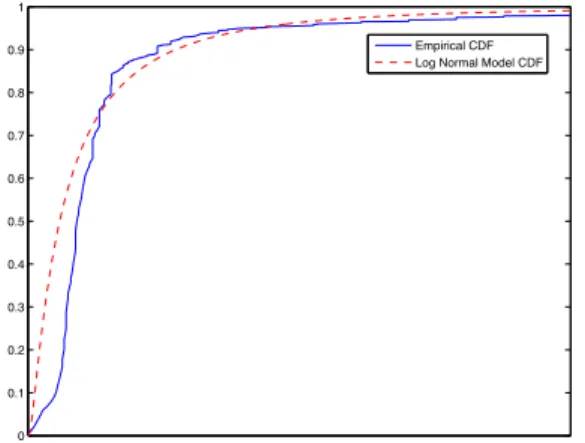
Figure 1: The observed and modeled distribution of the winning bid on the Right Media Exchange.
4.
EXPERIMENTS
In this section we evaluate our algorithms on syntheti-cally derived data drawn from a log-normal distribution, which fits data observed from the Right Media Exchange. Algorithms for the fully observable case are evaluated in Section 4.2, and the partially observable case in Section 4.3.
4.1
Methodology and Data
To evaluate our algorithms, we collected winning bids from live auctions run on the Right Media Exchange, which has over 50,000 buyers and sellers and processes over 6 bil-lion impressions daily. The bids we collected represent a 1% uniform sample across a variety of individual publish-ers. Focusing on a single publisher, we plot the CDF of the empirical distribution of the bids in Figure 1.
While it is difficult to predict the winning bid on any par-ticular impression, for a fixed publisher the data can be fitted with a log-normal distribution with the appropriate mean and variance. In Figure 1 we provide such a fit for a single publisher (350,000 auctions total). While the exact vari-ance changes from publisher to publisher, on all instvari-ances the data can be fitted well with a log-normal distribution.
Based on the above fit, we sample i.i.d. from a log-normal
distribution with mean and variance one.8 While very large prices are never observed on the exchange, the log-normal distribution supports arbitrarily large prices. We deal with this by discarding samples larger than an upper-limitb, cho-sen to be the 99.7thpercentile. That is, we sample from the log-normal distribution conditioned on{X≤b}.
We set the supply to ben= 10,000 impressions. To eval-uate each algorithm we choose 16 evenly spaced values of target f and targettfrom the interval (0,1), and measure the actual fraction and spend against the targets (we in-clude only 4 data points each for clarity). For each of the 256 parameter settings, we run each algorithm on 500 i.i.d. samples to average out effects of sampling.
4.2
Results: Fully Observable Exchange
TheLearn-Then-Bid algorithm waits for a significant ex-ploration period before bidding. An obvious improvement is theLearn-While-Bid algorithm which continues to learn during exploitation: Pm,Pm,? AmandZ?mare updated after
eachbid, as inLearn-Then-Bid lines 2–5 but with adaptive targets. Although harder to analyze, this has the advantage of a possibly shorter exploration phase without compromis-ing estimation accuracy. We compare the performance of these two algorithms experimentally: onaverageboth algo-rithms perform very close to ideal. However, Learn-While-Bid spending is moretightly concentrated around the ideal thanLearn-Then-Bid for the same exploration-only phase.
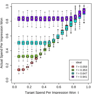
Figures 2 and 3 show the spending of Learn-Then-Bid
and Learn-While-Bid respectively. The dotted lines depict the minimum spending necessary to achieve the target frac-tion of supply as given by max{E[X|X≤z?], t}: when the
fraction and spend goals cannot simultaneously be satisfied, both algorithms prioritize the former while minimizing over spending. The distribution of each algorithm’s spending, for each (f, t) pair, is summarized by a box-and-whisker plot: each box depicts the 25%, 50% (the median) and 75% quan-tiles representing the spread of spending. As is evident in the figures, more runs of Learn-While-Bid have spend close to the ideal. To achieve comparable concentration with Learn-Then-Bid, mmust be increased. However this can lead to infeasibility for highf(e.g. form= 1,000 andf= 0.94 the problem becomes infeasible leading to underdelivery). Fig-ure 4 plots the performance of the algorithms with respect to supply. Both algorithms win close to the target fraction of supply for a wide range of target spending goals.
Figure 5 compares theory and practice, depicting our bou-nds on the concentration of the fraction of supply won and the spending per impression won, with respect to increasing exploration length. As exploration increases, the bounds become tighter but at the same time the problem becomes harder to satisfy until it becomes infeasible (occurring at the maximum mshown). Also shown are empirical results for runningLearn-Then-Bid. In particular for eachmvalue (exploration phase length), Learn-Then-Bid was run 1,000 times. For each run the fraction won during exploitation, and the spend per impression won, were calculated and the 95% two-sided quantiles were computed and overlayed. In this case the distribution-free theory matches the empirical results well, particularly for concentration of fraction won. 8We note that increasing the variance of the log-normal distribution does not affect our algorithms’ behavior; they deliver the same supply and actually overspend less (since there is a larger fraction of lower-priced impressions).
0.0 0.2 0.4 0.6 0.8 1.0 0.0 0.2 0.4 0.6 0.8 1.0
Target Spend Per Impression Won t
Actual Spend Per Impression Won
● ● ● ● ● ● ● ● ● ● ● ● ● ● ● ● ideal f = 0.059 f = 0.353 f = 0.647 f = 0.941 ●
Figure 2: Actual & ideal spend per impression won byLearn-Then-Bid withm= 100for 4values of f.
0.0 0.2 0.4 0.6 0.8 1.0 0.0 0.2 0.4 0.6 0.8 1.0
Target Spend Per Impression Won t
Actual Spend Per Impression Won
● ● ● ● ● ● ● ● ● ● ● ● ● ● ● ● ideal f = 0.059 f = 0.353 f = 0.647 f = 0.941 ●
Figure 3: Actual & ideal spend per impression won byLearn-While-Bid withm= 100for 4values of f.
0.0 0.2 0.4 0.6 0.8 1.0 0.0 0.2 0.4 0.6 0.8 1.0
Target Fraction of Impressions f
Attained Fraction of Impressions
LTB LWB t = 0.059 t = 0.353 t = 0.647 t = 0.941 ideal
Figure 4: Fraction of supply won byLearn-Then-Bid
and Learn-While-Bid withm= 100 for 4values oft.
1000 2000 3000 4000 0 1 2 3 4 5 6 7 Exploration Duration m
Spending Per Impression Won
0.0 0.2 0.4 0.6 0.8 1.0
Fraction Won During Exploitation
Ideal Theory Experiment Supply
Spend
Figure 5: Learn-Then-Bid supply and spend 95%
confidence bands given by: the concentration
bounds, and 1,000-sample empirical quantiles.
4.3
Results: Partially Observable Exchange
In this section we evaluate algorithms for bidding in a par-tially observable exchange. TheGuess-Double-Panic algo-rithm outperforms the strawman bidders in terms of target spend for a wide range of target supply fractions. More in-terestingly, the lack of full information does not handicap theGuess-Double-Panic algorithm: the accuracy of supply and spend are very close to those for full information.
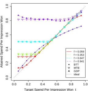
Figures 6 and 7 plot the supply and spend for Guess-Double-Panic as well as two strawman algorithms, Max-Then-Bid andBid-Two-t. Given thatLearn-Then-Bid per-forms well even for very short exploration phases, it is
natu-ral to apply the same idea in the partially observable setting:
Max-Then-Bidbidsbin the lengthmexploration phase and then exploits based on the empirical distribution.9
WhileMax-Then-Bidperforms well on supply it is an in-ferior strategy for target spend, since the spending during exploration can be very high: specifically whenf andtare both small the algorithm must acquire the right number of 9Max-Then-Bid dominates Learn-Then-Bid in number of impressions acquired despite partial information: Max-Then-Bid winseveryimpression during exploration in con-trast toLearn-Then-Bidwhich wins zero. Also, if the prob-lem is feasible after Learn-Then-Bid’s exploration then it will be feasible forMax-Then-Bid.
0.0 0.2 0.4 0.6 0.8 1.0 0.0 0.2 0.4 0.6 0.8 1.0
Target Fraction of Impressions f
Attained Fraction of Impressions
● ● ● ● ● ● ● ● ● ● ● ● ● ● ● ● ● ● ● ● ● ● ● ● ● ● ● ● ● ● ● ● ● ● ● ● ● ● ● ● ● ● ● ● ● ● ● ● ● ● ● ● ● ● ● ● ● ● ● ● ● ● ● ● ● t = 0.059 t = 0.353 t = 0.647 t = 0.941 BTT MTB GDP ideal
Figure 6: Fraction of supply won byBid-Two-t,
Max-Then-Bid and Guess-Double-Panic with m= 100for
4values of t. 0.0 0.2 0.4 0.6 0.8 1.0 0.0 0.2 0.4 0.6 0.8 1.0
Target Spend Per Impression Won t
Attained Spend Per Impression Won
● ● ● ● ● ● ● ● ● ● ● ● ● ● ● ● ● ● ● ● ● ● ● ● ● ● ● ● ● ● ● ● ● ● ● ● ● ● ● ● ● ● ● ● ● ● ● ● ● ● ● ● ● ● ● ● ● ● ● ● ● ● ● ● ● f = 0.059 f = 0.353 f = 0.647 f = 0.941 BTT MTB GDP ideal
Figure 7: Spend per impression won by
Bid-Two-t, Max-Then-Bid and Guess-Double-Panic with m=
100for 4values off.
impressions at a low price, andMax-Then-Bidis very likely to overspend. Guess-Double-Panic will perform well pre-cisely in this setting due to its more cautious exploration starting with a bid oft as opposed to b. This comparison is borne out in Figure 7 where Max-Then-Bid overspends most dramatically relative to Guess-Double-Panic for the lowest target fractionf= 0.059; overspending is evident for higher values up tof= 0.59. TheBid-Two-tstrawman al-gorithm does not perform much better than expected from theory, which predicts supply and spend within only a loose multiplicative factor of the targets.
5.
CONCLUSIONS
We study the problem of acquiring a given number of im-pressions with a given budget constraint by bidding against anunknown distribution. Our approach consists of learn-ing the distribution in an exploration phase, and then bid-ding accorbid-ding to the empirical distribution of observations from exploration. We consider both the fully observable and the harder partially observable case, and present algorithms with theoretical performance guarantees that also perform very well in experimental evaluations against realistic data. The experiments indicate that in addition to performing well with respect to both constraints, our algorithm for partial information does nearly as well as algorithms in the full in-formation setting despite the fact that a cost must be paid for every sample during exploration. The performance of the algorithms improves as the supply increases, and is asymp-totically optimal since a longer exploration phase can be used for higher accuracy; also, the actual number of impres-sions won and the total spend are more tightly concentrated around their means asnincreases.
The most interesting direction for further research is re-moving the i.i.d. assumption, and considering a game theo-retic perspective: we assume that every other bidder in each individual auction has unit demand and therefore bids his
value; one can instead consider best response and equilib-rium analysis when a number of bidding agents compete in such a marketplace.
Acknowledgements
We gratefully acknowledge the support of the NSF through grant DMS-0707060.
6.
REFERENCES
[1] P. Auer, N. Cesa-Bianchi, and P. Fischer. Finite-time analysis of the multi-armed bandit problem.Machine Learning, 47:235–256, 2002.
[2] M. Cary, A. Das, B. Edelman, I. Giotis, K. Heimerl, A. Karlin, C. Mathieu, and M. Schwarz. Greedy bidding strategies for keyword auctions. InEC ’07: Proceedings of the 8th ACM Conference on Electronic Commerce, pages 262–271, 2007.
[3] N. Cesa-Bianchi and G. Lugosi.Prediction, Learning, and Games. Cambridge University Press, 2006. [4] A. Dvoretzky, J. Kiefer, and J. Wolfowitz. Asymptotic
minimax character of the sample distribution function and of the classical multinomial estimator.Annals of Mathematical Statistics, 27(3):642–669, 1956. [5] N. Littlestone and M. K. Warmuth. The weighted
majority algorithm.Information and Computation, 108(2):212–261, February 1994.
[6] M. Zinkevich. Online convex programming and
generalized infinitesimal gradient ascent. InProceedings of the Twentieth International Conference on Machine Learning, pages 928–936, 2003.