An agent-based simulation model of structural change in agriculture

An Agent-Based Simulation

Model of Structural

Change in Agriculture

A Thesis

Submitted to the College of Graduate Studies and Research

in Partial Fulfillment of the Requirements

for the Degree of

Master of Science

In the Department of

Bioresource Policy, Business, and Economics

University of Saskatchewan

by

Peter C. Stolniuk

Permission to Use

In presenting this thesis in partial fulfillment of the requirements for a postgraduate degree from

the University of Saskatchewan, I agree that the Libraries of this University may make it freely

available for inspection. I further agree that permission for copying of this thesis in any manner,

in whole or in part, for scholarly purposes may be granted by the professors who supervised my

thesis work, or in their absence, by the Head of the Department or the Dean of the College in

which my thesis work was done. It is understood that any copying or publication or use of this

thesis or parts thereof for financial gain shall not be allowed without my written permission. It is

also understood that due recognition will be given to me and the University of Saskatchewan in

any scholarly use that may be made of any material in this thesis.

Requests for permission to copy or to make other use of the material in this thesis in whole or

part should be addressed to:

Head of the Department of Agricultural Economics

University of Saskatchewan

51

Campus

Drive

Abstract

Stolniuk, Peter, M.Sc. University of Saskatchewan, Saskatoon, March 2008.

An Agent-based Simulation Approach to Forecast Long-Run Structural Change in the

Saskatchewan Grain and Livestock

Sectors.

Supervisor: R.A. Schoney

Like many North American agricultural regions, Saskatchewan has experienced significant

fundamental structural changes in farming. Structural change encompasses evolution in

distribution of farm sizes, land tenure and financial characteristics, as well as variations in

demographic and production characteristics. These issues are often a source of discontent among

farm populations as it implies these populations are forced to adapt in a number of potentially

unpleasant ways. These changes have profound and sometimes poorly understood effects on the

rural economy – for example, structural change affects rural population and therefore demand for

rural infrastructure.

Traditional agricultural farm level analysis is often conducted using a representative farm or

group, but this framework cannot capture the growing heterogeneity of modern farm operators or

the current operating environment in agricultural regions. Farm profiles vary by demographic

characteristics, such as age and education, and resource endowments. Agent-based simulation

captures this heterogeneity through a farm by farm analysis, where after initialization, the

regional economy evolves over time.

A synthetic population is created based on survey data and the land characteristics based on the

actual land data in CAR 7B of Saskatchewan. A number of different price and yield time paths

were created using a bootstrap procedure on historical data and the model evolved to potential

agriculture structures that may occur in the model region, 30 years in the future.

Structural change occurs endogenously as farms interact in land markets, and make decisions on

land use. Agents compete for available land in a purchase and lease market with land selling to

the highest bidder. The dynamic nature of agent-based models allows individual farms to adjust

land use in response to changing economic conditions and individual preferences. How

The results indicate that many of the trends are the same under the different price and yield time

paths, however the rate of change is significantly impacted by the price and yield time path that

occurs. The model predicted the trend to fewer and larger farms will continue into the future.

The forecasted distribution of smaller farms will decline and proportion of large farms will

increase, while mid sized farms will remain relatively unchanged. The proportion of mixed

farms, land use, and total livestock numbers depend significantly on the price and yield time path.

The actual structure that will occur will be the result of the actual individual price and yield time

path that occurs.

Acknowledgements

As I look back many people have contributed to the success of this thesis. I would first like to

thank my supervisor Dr. Richard Schoney for his time, patience, knowledge, and encouragement.

I am extremely grateful that his door was always open and that he was willing to discuss any

issues that I encountered. Next, I would like to thank committee member Dr. James Nolan, for

the advice, comments, and enthusiasm in this area of research, as well as the very much

appreciated words of encouragement along the way. I would also like to thank committee

member Dr. Craig Wilson and external examiner Dr. James Unterschultz for helpful comments

that significantly benefited this research. I would like to thank my classmates who offered a

much needed break from research. I owe a great deal of gratitude to my parents who instilled the

value of education in me and for their support throughout not only this process, but in all other

aspects of my life. Lastly, my wife Karyn for her support throughout my years as a graduate

student, without you this would have never been possible.

Table of Contents

Permission to Use ... i

Abstract... ii

Acknowledgements ... iv

Table of Contents ...v

List of Figures... viii

List of Tables ...x

Chapter 1 ...1

1.0 Introduction

...1

1.2 Objectives and Expected Results

...2

1.3 Thesis Organization

...3

Chapter Two...4

2.0 Introduction

...4

2.1 What is Agent-based Modeling?

...4

2.1.1 Advantages of Agent-based Models

...5

2.1.1.1 Complexity

...5

2.1.1.2 Flexibility

...6

2.1.1.3 Emergence

...6

2.1.1.4 Spatial Representation, Soil Quality and Land Use

...6

2.2 Causes of Structural Change

...7

2.2.1 Technology and Economies of Size

...7

2.2.2 Off Farm Employment and Demographic Characteristics

...8

2.3 Land Use

...9

2.3.1 Land Use Methodologies

...10

2.3.1.1 Equation Models

...10

2.3.1.2 Agent-based Models of Land Use

...11

2.3.2 Land Use Decisions

...11

2.4 Agent-based Models of Structural Change

...12

2.5 Farmland Markets

...12

2.5.1 Farmland Bid Value

...13

2.5.1.1 Market Based Annual Rent

...13

2.5.1.2 Government Payments

...14

2.5.1.3 Capital Gains

...14

2.5.1.4 The Role of Capital and Liquidity Constraints

...14

2.5.2 The Role of Speculation

...15

2.5.3 Farmland Leasing

...15

2.5.4 Farmland as an Investment

...16

2.6 Forage Markets

...16

2.7 Summary

...17

Chapter 3 ...18

3.0 Introduction

...18

3.1 NetLogo

Platform

...19

3.2 Heterogeneity

...19

3.2.1 Agent Heterogeneity

...20

3.2.2 Land Heterogeneity

...20

3.3 Dynamics

...21

3.3.1.1 Cost of Production

...22

3.3.1.2 Land Use

...23

3.3.1.3 Incomplete Information

...23

3.5 Summary

...24

Chapter 4 ...25

4.0 Introduction

...25

4.1 Model Assumptions

...26

4.2 Farm Production Activities

...27

4.2.1 Crop Income

...27

4.2.2 Forage and Livestock Production

...28

4.2.2.1 Livestock Income

...28

4.2.2.2 Hay and Pasture Production

...29

4.2.2.3 Hay and Pasture Usage

...30

4.2.2.4 Hay Reserves, Sales, and Purchases

...31

4.2.3 Variable Costs and Forage Establishment and Breaking

...32

4.2.4 Transportation Expense

...32

4.2.5 Annual Machinery Repairs

...33

4.2.6 Cash Commitments

...34

4.3 Off Farm Employment and Family Living Withdrawal

...34

4.4 Farm Accounting

...35

4.4.1 Cash Flows

...35

4.4.2 Balance Sheet

...35

4.5 Farm Agent Expectations

...36

4.6 Farm Agent Crop Mix

...37

4.7 Farm Exits and Transfers

...37

4.8 Land Use

...38

4.9 Machinery and Livestock Investment

...41

4.10 Farmland Markets

...42

4.10.1 Bidding Eligibility Criteria

...43

4.10.2 Farmland Purchase Market

...44

4.10.2.1 Maximum Bid Based on Income Earning Ability

...44

4.10.2.3 Investor’s Bid Value and Minimum Acceptable Price

...48

4.10.3 Auction Process

...50

4.10.4 Farmland Lease Market

...50

4.10.4 Lease Renegotiation

...51

4.11 Summary

...51

Chapter 5 ...52

5.0 Introduction

...52

5.1 Synthetic Farm Population

...53

5.1.1 Farm Size, Operator Age, and Off Farm Income

...53

5.1.2 Land Tenure, Land Use, and Livestock Numbers

...54

5.1.3 Assets and Debt

...55

5.2 Stochastic Prices and Yields

...56

5.3 Crop Production Data

...58

5.3.1 Crop Variable Cost

...58

5.3.2 Crop Machinery Options

...59

5.4 Livestock and Forage Production Data

...61

5.4.1 Cow and Forage Variable Costs

...61

5.4.2 Livestock Energy Requirements and Energy from Various Feed Sources

...62

5.4.3 Forage Establishment and Breaking Costs

...63

5.4.4 Forage Reserves and Transaction Fee

...64

5.5 Transportation Costs

...64

5.6 Hired Labour Costs

...64

5.7 Retirements and Farm Transfers

...65

5.8 Family Living Withdrawal

...66

5.9 Model Validation

...67

5.10 Summary

...68

Chapter 6 ...69

6.0 Introduction

...69

6.1 Simulation Results: Base Scenario

...69

6.1.1 Farm Numbers, Type, and Average Size

...69

6.1.2 Distribution of Farm Sizes

...73

6.1.3 Land Use, Total Livestock Numbers, and Average Herd Size

...75

6.1.4 Financial Characteristics

...78

6.1.4.1 Farm Financial Characteristics

...78

6.1.4.2 Financial Characteristics by Farm Type

...81

6.1.5 Land Markets

...82

6.1.5.1 Farm Exits

...82

6.1.5.2 Land Price and Lease Rate

...82

6.1.5.3 Land Tenure

...83

6.1.5.4 Unfarmed Land

...84

6.2 Simulation Results: Alternative Scenarios

...85

6.2.1 Farm Numbers, Type, and Average Size

...85

6.2.2 Distribution of Farm Sizes

...88

6.2.3 Land Use, Livestock Numbers, and Herd Size

...90

6.2.4 Financial Characteristics

...92

6.2.4.1 All Farms Financial Characteristics

...92

6.2.5 Land Markets

...95

6.2.5.1 Farm Exits

...96

6.2.5.2 Land Price and Lease Rate

...96

6.2.5.3 Land Tenure

...97

6.3 Summary

...97

Chapter 7 ...99

7.1 Summary

...99

7.2 Conclusions

...100

7.3 Limitations

...101

7.4 Suggestions for Further Study

...102

References...103

Appendix A...110

Appendix B ...112

Appendix C...114

Appendix D...115

Appendix E ...117

List of Figures

Figure 3.1:

Conceptual Model of an agricultural system...19

Figure 3.2:

Farmland Markets...21

Figure 3.3:

Average Cost of Production with Lumpy Investments ...22

Figure 4.1:

Annual Farm Agent Activities...25

Figure 5.1:

Census Agriculture Regions of Saskatchewan ...52

Figure 5.2:

Historic Land Prices and Simulated Land Prices ...68

Figure 6.1:

Simulated Farm Numbers (Base Scenario) ...70

Figure 6.2:

Simulated Distribution of Final Farm Numbers (Base Scenario)...70

Figure 6.3:

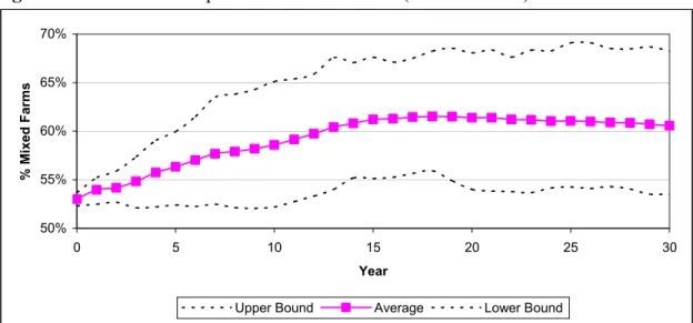
Simulated Proportion of Mixed Farms (Base Scenario)...71

Figure 6.4:

Simulated Mean Farm Size (Base Scenario) ...71

Figure 6.5:

Simulated Distribution of Final Mean Farm Size (Base Scenario) ...72

Figure 6.6:

Simulated Mean Farm Size by Farm Type (Base Scenario) ...73

Figure 6.7:

Simulated Distribution of All Farm Sizes (Base Scenario)...73

Figure 6.8:

Simulated Distribution of Grain Farm Sizes (Base Scenario)...74

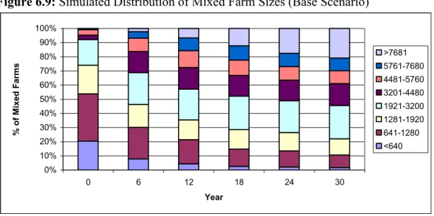
Figure 6.9:

Simulated Distribution of Mixed Farm Sizes (Base Scenario)...75

Figure 6.10:

Simulated Proportion of Land Used in Crop Production (Base Scenario) ...75

Figure 6.11:

5 Simulated Time Paths of Proportion of Land Used in Crop Production (Base

Scenario)...76

Figure 6.12:

Simulated Mean Mixed Farm Herd Size (Base Scenario)...77

Figure 6.13:

Simulated Total Cow Herd Size (Base Scenario)...77

Figure 6.14:

Simulated Distribution of Mixed Farm Herd Sizes (Base Scenario)...78

Figure 6.15:

Simulated Mean Net Worth (Base Scenario) ...79

Figure 6.16:

Simulated Distribution of Final Mean Net Worth (Base Scenario)...79

Figure 6.17:

Simulated Mean Debt to Assets (Base Scenario) ...80

Figure 6.18:

Simulated Distribution of Final Mean Debt to Assets (Base Scenario) ...80

Figure 6.19:

Simulated Mean Net Worth by Farm Type (Base Scenario)...81

Figure 6.20:

Simulated Mean Debt to Assets by Farm Type (Base Scenario) ...81

Figure 6.21:

Simulated Land Price (Base Scenario) ...83

Figure 6.22:

Simulated Land Lease Rate (Base Scenario)...83

Figure 6.23:

Simulated Proportion of Leased Land (Base Scenario)...84

Figure 6.24:

Simulated Farm Numbers (All Scenarios)...85

Figure 6.25:

Simulated Proportion of Mixed Farms (All Scenarios)...86

Figure 6.26:

Simulated Mean Farm Size (All Scenarios) ...86

Figure 6.27:

Simulated Mean Grain Farm Size (All Scenarios) ...87

Figure 6.28:

Simulated Mean Mixed Farm Size (All Scenarios)...88

Figure 6.29:

Simulated Distribution of All Farm Sizes (Scenario 1)...89

Figure 6.30:

Simulated Distribution of All Farm Sizes (Scenario 2)...89

Figure 6.31:

Simulated Proportion of Land Used in Crop Production (All Scenarios) ...90

Figure 6.32:

Simulated Mean Total Cow Herd Size (All Scenarios)...91

Figure 6.33:

Simulated Mean Mixed Farm Herd Size (All Scenarios)...91

Figure 6.34:

Simulated Mean Net Worth (All Scenarios)...92

Figure 6.35:

Simulated Average Debt to Assets (All Scenarios)...93

Figure 6.36:

Simulated Mean Grain Farm Net Worth (All Scenarios) ...93

Figure 6.37:

Simulated Mean Mixed Farm Net Worth (All Scenarios)...94

Figure 6.38:

Simulated Mean Grain Farm Debt to Assets (All Scenarios)...95

Figure 6.40:

Simulated Land Price (All Scenarios) ...96

Figure 6.41:

Simulated Land Lease Rate (All Scenarios)...97

List of Tables

Table 5.1:

Initial Distribution of Farms by Age and Farm Size (Synthetic Population)...54

Table 5.2:

Distribution of Off Farm Income by Farm Size (Synthetic Population)...54

Table

5.3:

Initial Land Tenure, Land Use, and Cow Numbers ...55

Table 5.4:

Distribution of Farm Debt by Age (Synthetic Population) ...56

Table 5.5:

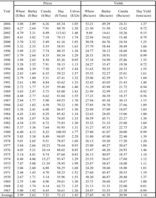
Historic Yields and Detrended Prices ...58

Table 5.6

: Variable Cost per Acre of Various Cropping Alternatives ...59

Table 5.7:

Crop Machinery Options...60

Table 5.8:

Farmers Crop Mix ...60

Table 5.9:

Cow Production Variable Costs Excluding Labour and Feed ...61

Table 5.10:

1,300 lb beef cow Energy requirements as predicted by CowBytes

...62

Table 5.11:

Forage Seeding and Breaking Cost for the Dark Brown Soil Zone...63

Table 5.12:

Crop Enterprise Hired Labour...65

Table 5.13:

Probability of Farm Exits by Farm Operator Age...66

Table 5.14:

Probability of Off Farm Employment by Farm Size...66

Table 6.1:

Farm Exits by Exit Type (Base Scenario)...82

Chapter 1

Introduction

1.0 Introduction

Modern economies continually experience structural change as new technologies, policies, and

markets emerge or change. For some people it results in discontent as they are forced to change,

relocate, or adjust to lower earnings. This is evidenced by the debate about what the future holds

for the “family farm” and the role of agricultural policy in determining that future. For others

structural change can be viewed as a challenge that creates new market opportunities.

The changing structure of agriculture is often characterized by the decline in farm numbers

accompanied by the increase in farm size. Goddard et al. (1993) identifies structural change as

changes in essential characteristics of production activities. Therefore, structure of an industry

can also include: 1) farm size and distribution 2) technology and production characteristics 3)

demographic characteristics, and 4) resource ownership and financing. Changes in farm size and

distribution are based on the number of farms in each size category. The production mix and

how these products are produced are influenced by technology and production characteristics.

Demographic characteristics include the age, education, and financial characteristics of farm

operators. Land tenure, whether land is leased or owned, and how land and other assets are paid

for is included in resource ownership and financing.

The farming sector is characterized by many different individuals with different financial and

demographic characteristics. Traditional economic models, such as general or partial equilibrium

models, are unable to capture the diversity and interactions apparent in agriculture system and

cannot accurately forecast behaviour far beyond the years which the model parameters where

derived (Freeman 2005). This has led researchers to utilize alternatives to traditional economics

such as, agent-based modeling, when analyzing structure of the agricultural industry.

Public programs can have a significant impact on the agricultural structure. Agricultural policies

can impede or encourage structural change by increasing the profitability of one production

activity relative to others, resulting in an inefficient allocation of resources (Happe 2004).

Agricultural support programs also create an incentive for inefficient producers to remain in

operation by subsidising their income to an acceptable level (Happe 2004), slowing agricultural

adjustment. As a result the direct costs and benefits of public programs interfere with the process

of structural change in an economy (Goddard et al. 1993). It is critical that policy makers have

the ability to accurately evaluate the impacts of agricultural policy both in the short run and many

years into the future.

The structure of agriculture is an important issue because it has a large impact on rural

communities. Fewer and larger farms lead to rural depopulation, which has an impact on the

demand for infrastructure. With fewer people in rural areas there is less demand for schools,

hospitals, recreational facilities, roads, and businesses and services in these areas. Closing of

these businesses and services leads to concern of the remaining population of the rural areas and

may feedback and influence their decision to remain in the rural area. The structure of

agriculture also impacts the type and location of processing facilities, which can impact the

marketing and production plans of producers.

1.2 Objectives and Expected Results

The primary purpose of this research is to project what the future agricultural structure in

Saskatchewan will be in 30 years under alternative price scenarios. More specifically the farm

numbers, farm size and distribution of size, production characteristics, demographic

characteristics, and resource ownership and financing of the agricultural industry will be

projected. This is achieved through expanding the agent-based model of Freeman (2005) to

represent typical Census Agriculture Region in Saskatchewan, where structural change takes

place endogenously within the model. Freeman’s model was expanded to include: 1) mixed

farms that are willing to use land in the highest and best use to produce forage and livestock or

annual crops in addition to grain farms unwilling to produce livestock and 2) economies of size

and lumpy machinery investments for the annual crop production enterprise. The inclusion of

livestock allows farmers to make annual land use decisions and expected land use when creating

bid values in the farmland markets based on profitability, with mixed farms having a bidding

advantage on land suited for livestock production. The model is initialized with an exogenous

price scenario and is allowed to evolve over time revealing the future agricultural structure.

It is expected that the price and yield scenarios will have an important role on the structural

change that occurs. If the prices and yields are high it is likely that the farm numbers will not

decline as quickly as a scenario with lower prices and yields. However, it is possible that the

increase in income could be captured by the individuals selling and leasing land in the land

markets and not have a significant impact on farm numbers. It is also expected that if the relative

price of livestock increases to annual crops, the mixed farms will have a bidding advantage in the

land markets and will likely increase farm size while grain farms may eventually be forced to exit

the industry.

1.3 Thesis Organization

This thesis is composed of seven chapters. Chapter two is a brief discussion of the literature on

agent-based models and their suitability to modeling a complex agricultural system, causes of

structural change, farmland markets and bid values, land use, and forage markets. The following

chapter develops a conceptual model of an agricultural system. The fourth chapter defines in

detail the individual agents’ behaviour. The fifth chapter outlines the model initialization and

data, followed by a chapter describing the results. The last chapter contains summary and

concluding remarks.

Chapter Two

Literature Review

2.0 Introduction

This chapter will review the literature that applies to modeling agricultural structural change.

The first section deals with agent-based models and their advantages, including the ability to

handle complex systems, build models at the individual level, produce emergent or unexpected

results, and capture heterogeneity and spatial characteristics. This is followed by a discussion on

how technology and economies of size, off farm employment, and demographic characteristics

affect structural change. A discussion of the characteristics of equation models and agent-based

models of land use and the factors that influence the land use decision follows. Next, a section

focusing on other agent-based studies of structural change and their suitability to a Saskatchewan

agricultural system. Following this, a discussion on how farmer’s determine farmland bid values,

from annual income, government payments, capital gains, and capital and liquidity constraints.

Also included in this section is a discussion on the role of speculation in the farmland markets,

description of farmland leasing, and farmland as an investment for non-farming individuals.

There is then a brief discussion on forage markets, followed by a summery of the chapter.

2.1 What is Agent-based Modeling?

Agent-based modeling (AbM) is a relatively new methodology to economics (Rosser 1999), but

it is an established methodology in other social science (Parker et al. 2003). AbM consists of

autonomous, interacting agents who make decisions linking their behaviour to the environment

(Parker et al. 2003). These models are computer simulations of individual agents used to study

how their aggregation leads to complex macro behavior (Berger 2001). Increases in computing

power have allowed increasingly complex problems to be analyzed using AbM.

Agent-based modelers initialize an economy with a population of agents distributed across a

geographical landscape (Tesfatsion 2002). Common behavioral and decision rules are assigned

to all agents, but each individual agent can vary according to demographic, financial, and other

personal characteristics. Once the decision rules and initial attributes of the agents are set and

exogenous data included, there is no further intervention by the modeler and the economy

evolves over time (Tesfatsion 2002).

2.1.1 Advantages of Agent-based Models

AbM offers a number of advantages over traditional economic models. Freeman (2005) identifies

some of these as: 1) the ability to obtain numerical solutions in complex systems that maybe

unsolvable analytically, 2) flexibility, 3) emergent characteristics, and 4) spatial representation.

AbM’s ability to capture these characteristics gives it potential to overcome the limitations of

previous farm level models (Freeman 2005) and include aspects such as heterogeneity and

feedback that exist in an agricultural system.

2.1.1.1 Complexity

Agricultural economists have viewed agricultural structures as complex dynamic systems since

the 1960s (Happe 2004). Complex systems are characterized by heterogeneity,

interdependencies, and nested hierarchies among agents and their environment (Parker et al.

2003). Heterogeneity includes both differences in agents and land characteristics. Agents vary

according to demographic characteristics, financial characteristics, and available resources. Land

is heterogeneous in terms of soil quality, which can influence land use, farmable area and

location. Interdependencies arise because agents rely on information from their past decisions and

other agents’ decisions to update their decision making strategy (Parker et al. 2003). An example

of interdependencies in an agricultural region is the land market, where a farm is unable to

expand unless another agent decides to sell (Happe 2004). Hierarchal structures occur as

individuals interact to form households, which interact with other households to form villages,

with multiple scales influencing individual agents (Parker et al. 2003). Rosser (1999) adds that in

economics, an added layer of complexity results from interacting human calculations in decision

making, which may not exist in other disciplines.

2.1.1.2 Flexibility

The flexibility of AbM allows for a “bottom up” approach to modeling that does not rely on

exogenous assumptions that are required by “top down” approaches (Freeman 2005). Traditional

equilibrium models require fixed decision rules, common knowledge assumptions, representative

agents, and imposed market equilibrium constraints (Tesfatsion 2002). These assumptions are

required to ensure consistency between the macro and micro level (Happe 2004). Once the

mechanics of an AbM are understood and programmed, the researcher has greater flexibility to

design and execute experiments to explore alternative causal mechanisms that are more complex

and possibly easier to solve than equilibrium based solutions (Parker et al. 2003). In AbM’s there

are no market equilibrium constraints allowing the market to be out of equilibrium.

2.1.1.3 Emergence

The interactions of a complex system may give rise to emergent phenomenon. There are

numerous definitions of emergence in the literature, but there are some commonalities. Gilbert

and Troitzsch (2002) state a phenomenon is emergent if it requires new categories to describe it,

which are not required to describe the behavior of the underlying components. Many of the

definitions concern macro scale phenomena that arise as a result of complex, micro-scale

interactions (Parker et al. 2003). Other definitions associate emergence with surprise or

unanticipated results (Batty and Torrens 2001). An early example of emergence is in Schelling’s

(1978) model of how nieghbourhoods become segregated by race. Schelling found that a

moderate urge to avoid being the minority in a particular neighbourhood results in highly

segregated nieghbourhoods to develop.

2.1.1.4 Spatial Representation, Soil Quality and Land Use

Spatial representation is an important aspect of agriculture because it can have a significant

impact on farm level decisions. An example is the transportation costs associated with

machinery operations and its affect on farming geographically dispersed land (Freeman 2005).

Transportation costs from farmstead to field increase with distance causing competition for land

to be mainly between neighbours (Berger 2001).

Soil quality is often associated with certain geographical features such as glacial moraines, river

deltas, ancient lake bottoms, or natural prairie/forest ecosystems. Production and land use

decisions are based on soil quality and consequently, the difference in soil quality determines the

spatial land use landscape (Berger 2001). AbM’s have the ability to capture spatial

characteristics, which are important to the agricultural structure.

2.2 Causes of Structural Change

Structural change is well documented in the literature. Although there is consensus that

structural change has occurred in the form of decreasing farm numbers and increasing farm size,

there often is no common agreement on the implications of these changes for the viability of the

sector, rural community, environment, and society (Goddard et al. 1993). In order to understand

the implications of structural change it is important to understand its underlying causes. The

following section reviews possible causes of structural change such as technology and economies

of size, off farm employment and demographic characteristics, and sectoral heterogeneity.

2.2.1 Technology and Economies of Size

A well known theory on possible cause of structural change is based upon Cochrane’s

technological treadmill. Cochrane (1958) maintained that new technology decreases the unit cost

of production and early adopters of this technology realize increased net incomes. As the number

of adopters increases, total output increases, resulting in lower prices, forcing other farmers to

adopt the technology to remain competitive. Those who do not adopt the technology are forced

out of the industry and their assets will be acquired by the producers that remain (Harrington and

Reinsel 1995). The result is that each individual has incentive to adopt the new technology, even

though their collective decision will not make them better off and could make them worse off

(Harington and Reinsel 1995).

Another cause of structural change is the presence of economies of size. Economies of size

imply that an increase in size will result in a decrease in the average total costs and therefore,

large farms are more efficient then small farms. Optimal farm size is the minimum of the

long-run cost curve (Goddard et al. 1993) and if an individual is not at this point there is incentive to

adjust farm size or resource use to reach this point. Technological change shifts this curve to the

right, increasing the number of farms with increasing returns to size and therefore increasing the

number of farms with incentive for farm growth (Goddard et al. 1993).

The shape of the long-run cost curve has important implications on the desire for farm growth.

Schoney (1997) identifies that the majority of studies find an “L shaped” curve where after a

threshold point most economies of size are exhausted. This threshold for grains and oilseeds was

estimated by Fleming and Uhm (1982) to be approximately 350 tonnes of production in the black

soil zone of Saskatchewan. Schoney (1997) estimated this threshold to be 1,500 to 2,000 acres in

the black soil zone and 2,500 to 3,000 acres in the brown soil zone of Saskatchewan. There is

little evidence of diseconomies of size in the literature (Schoney 1997), which creates incentive to

increase in size to obtain higher total returns even though cost will not decrease (Goddard et al.

1993).

2.2.2 Off Farm Employment and Demographic Characteristics

Structural change in agriculture can occur as a result of the ability for farm operators to use their

labour to earn off farm income. Farmers optimize their economic well being through allocating

their land, labour, and capital to farm and non farm uses (Harrington and Reinsel 1995). Kesliv

and Peterson (1982) believed a rise in urban incomes creates incentive to leave agriculture,

leaving the remaining land to fewer, but larger farms. With more resources, the remaining farms

increase their incomes, closing the urban-rural income gap (Kesliv and Peterson 1982).

Others have argued that off farm employment helps ensure the survival of smaller farms. Off

farm employment reduces the amount of farm income that is needed to meet a required standard

of living (Goddard et al. 1993). Increases in productivity and a fixed land base along with the

seasonal nature of agriculture causes farm families to have their available labour underemployed

(Olfert 1992). This allows for the reallocation of excess labour to off farm activities, raising their

household income. While once considered a transition phase for new entrants or a short-term

crisis response, off farm employment is now recognized as a stable long term condition (Olfert

1992). The increase in off farm employment has increased the number of small part time farmers

(Goddard et al. 1993).

Changing patterns of entry, growth, and exit can result in structural change (Harrington and

Reinsel 1995). This theory is known as the life cycle hypothesis. The life cycle hypotheses is

based on an agricultural ladder where operators enter through the renting of farm assets, add

more rented land for part of their lives, progressively acquire ownership of land, and finally

progressively relinquish control of rented and owned land during the exit stage (Harrington and

Reinsel 1995). Different age cohorts experience similar patterns that are marginally affected by

economic conditions, government policy, or external shocks (Harrington and Reinsel 1995).

Traditionally, farming entrants are young males that were raised on farms. However, this group

is shrinking in size as a result of fewer farms and declining birth rates (Gale 1993). Fewer

entrants implies continued aging of the current farm operators and fewer, larger farms (Gale

1993). Gale (1993) suggests that due to the fewer potential entrants, the number and size

distribution of farms may not reach equilibrium even if returns from non farm employment were

equivalent to farming.

There are a number of arguments on the causes of structural change in agriculture with little

consensus on the issue. The next section will review various land use methodologies and the

land use decision, which can influence structure.

2.3 Land Use

Land use denotes the human employment of the land (Meyer and Turner 1992). The land use

decision of an individual farmer will impact the level of income they are able to generate from

their available resources. Each individual’s land use decision is important in determining farm

profitability and survival. The income generated from land can also have an impact on the desire

for farm growth and the ability to bid for additional farmland.

Land use decisions not only impact the income of farmers, but also the location of infrastructure.

Processing facilities and services will locate in regions that have a large production of a specific

product. For example, in order to minimize travel and transportation costs, a veterinarian will

locate in a region that has large number of livestock and not in an area that is strictly grain and

oilseed farms. Infrastructure location can also feed back and impact land use decisions. If there

is a veterinarian in the area, a farmer will be more willing to switch land from grain and oilseed

to livestock production. The land use of each individual will therefore have a significant impact

on the structure of agriculture.

2.3.1 Land Use Methodologies

There are a number of methodologies used to analyze land use. Parker et al. (2003) identifies the

following models: 1) system models, 2) statistical techniques, 3) expert models, 4) evolutionary

models, 5) cellular models, and 6) agent-based models. This section will focus on equation

modeling and agent-based models of land use.

2.3.1.1 Equation Models

Most models are mathematical in some way, but some are especially so, that models rely on

equations that seek a static or equilibrium solution (Parker et al. 2003). One of these models is

the computable general equilibrium model (CGE). The CGE model has been used for land use

studies by Darwin et al. (1996), Ianchovichina, Darwin, and Shoemaker (2001), and Wong and

Alavalapati (2003).

CGE models are based on general equilibrium theory and assumptions. These assumptions

include perfect competition, full employment of resources, perfectly mobile factors of

production, complete information, and market clearing conditions (Scriecu 2005). CGE models

usually cover economy wide impacts on resource allocation and income, but at a very aggregate

level (Scriecu 2005). As a result, CGE models are weak at assessing and predicting the effects

across various households (Scriecu 2005).

To achieve analytical or computational tractability, equation models require simplifying

assumptions (Parker et al. 2003). Due to the highly aggregated results and the restrictive

assumptions of these types of models, the implications of a shock at the farm level may not be

accurately represented.

2.3.1.2 Agent-based Models of Land Use

A number of researchers have utilized AbM for analyzing land use (See Evans and Kelly 2004;

Kelly and Evans 2005; Balmann 2000; Huigen 2004; Robinson 2003). Land use AbM consist of

two components: 1) a cellular component that represents biophysical and ecological aspects of

the model and 2) an agent component that represents human decision making (Parker et al. 2003).

Traditionally land use models have incorporated biophysical attributes, such as soil quality as

primary land use determinants and have emphasized human decision making as having a smaller

role (Veldkamp and Lambin 2001). However, it is likely that human decision making plays a

role and is evidenced by the fact that land with similar attributes is often used differently (Kelly

and Evans 2005). Land use decisions are made by the individual household or owner of the land

and to understand land use requires learning about how private owners make decisions (Koontz

2001, Messina and Walsh 2001). Individuals make land use decisions based on constraints that

they face (Messina and Walsh 2001).

2.3.2 Land Use Decisions

The most common theory of land use decisions is based on the individual who is primarily

motivated by economic and financial returns (Koontz 2001). Any parcel of land is assumed to be

put its highest and best economic use, given its attributes and location (Lambin, Geist, and Lepers

2003).

Farming, haying, and grazing are primarily motivated by economic return, however many other

land use activities are motivated by other factors (Koontz 2001). Hosier (1988) maintains that

land use decisions are based on economic, environmental, aesthetic, and personal reasons. In

addition to economic reasons, Koontz (2001) identifies that non-monetary benefits may play a

large role in land use decisions. Based on interviews with land owners, Koontz (2001) found that

80% of individuals largely base their land use decisions on non-monetary benefits including

aesthetics, hobbies, and recreation. Non-monetary benefits vary across activity type, parcel size,

and land owner characteristics (Koontz 2001). Varying land use may be caused by

heterogeneous preferences. In the model developed by Kelly and Evans (2005), agents maximize

their expected utility from various activities by choosing how to allocate their labour and land. In

their model, utility is the weighted sum of expected pecuniary and non pecuniary aspects of each

activity. Each activity is assigned a preference weighting that can be different for different

agents. Kelly and Evans (2005) results indicate that land owners’ preferences are equally or

more important than land suitability for determining land use.

2.4 Agent-based Models of Structural Change

Agent-based models of structural change view agriculture as a complex system. One of the first

models was developed by Balmann (1997) for a hypothetical region in Germany, where structural

change occurred endogenously in the model. Largely based on the original model of Balmann

(1997), the AgriPoliS model subsequently developed by Balmann, Happe, and Kellermann was

used to analyze a number of agricultural policies and their impact on structural change (See

Happe 2004; Happe and Balmann 2003; Happe, Kellermann, and Balmann 2006; Sahrbacher et al

2005). However, the AgriPoliS model does not include some aspects which are important to

Saskatchewan agriculture. Farm growth in the AgriPoliS model is limited to producers renting

land as opposed to purchasing (Happe, Balmann, and Kellerman 2004). Another shortcoming of

this model is that it does not include a forage market, limiting livestock herd size.

Building upon the AgriPoliS model, Freeman (2005) developed a model to analyze differing

management styles and their impact on farm structure in Saskatchewan. Freeman’s model

enhanced the AgriPoliS model to include a land purchase market in addition to a lease market.

The land market included both a purchase market and a leasing market. This model imposes the

assumption that all farmers prefer to purchase land first and will lease land only if unsuccessful in

the purchase market. Freeman’s model had simulated results for the period of 1960 to 2000,

which replicated the actual structural change that occurred over the same period, validating AbM

as a methodology for predicting structural change. However, Freeman’s model does not include

economies of size, the ability to change land use, or livestock, which are important aspects of

Saskatchewan agriculture.

2.5 Farmland Markets

In Saskatchewan, farmers are able to gain control of additional farmland through a primary land

purchase market and a secondary leasing market. Farmland markets are characterized by: 1) few

buyers and sellers, 2) farmland rarely being sold, often averaging only once a generation, 3) a

relatively localized market, where competition is traditionally between neighbours, and 4)

imperfect information. To reach economies of size or increase profitability, farmers must

compete in farmland markets to gain control of additional farmland. Once a farmer gains control

of a parcel of land they can then make decisions on the best use of the land.

The following section will deal with some of the issues related to farmland markets. There will

be a brief discussion on the influences of farmland bids. This will be followed by the possibility

of speculation in the farmland markets. The remainder of this section will be a discussion on

farmland leasing and non farm operators investing in farmland.

2.5.1 Farmland Bid Value

The current value of farmland is the present value of the expected future economic return to land

(Pederson 1982). There have been a number of past studies that have attempted to identify major

sources of farmland value. Important sources of farmland value are: 1) market based annual rent,

2) government payments, and 3) capital gains. There has also been discussion on the possibility

of speculation in the farmland market, where individuals believe that the value of farmland will

likely increase in the future. This would cause the bid values of these individuals to increase as a

result of the expected capital gain.

2.5.1.1 Market Based Annual Rent

The underlying source of farmland value is the annual income it can generate (Burt 1986).

Rensiel and Rensiel (1979) thought that the changes in land values are a result of the changing

expectations that individuals have about the annual income. Alston (1986) found that most of the

real growth in land price can be accounted for by growth in real income. Although changes in

annual income are an important component in farmland valuation, they are not the only cause of

the changes in farmland price. Land prices tend to rise faster than income when both are rising

and fall faster when both are falling (Melichar 1979; Clark, Fulton, and Scott 1993). This has

lead to other theories of the causes of change in farmland values.

2.5.1.2 Government Payments

In Saskatchewan, a portion of annual farm income is made up of government support, paid to

farm operators. The size of these payments impacts the maximum bid of each individual farmer.

The level at which the government payments are capitalized into the bid value depends upon the

level of certainty that the support will continue in the future (Goodwin and Otalo-Magne 1992).

The level of support capitalized into land values has not been agreed upon in the literature. Moss,

Shonkwiler, and Reynolds (1989) believed that in the short run, an increase in government

support may signal future problems in agriculture and result in a decline in real asset values.

Both Turvey et al. (1995) and Goodwin and Ortalo-Magne (1992) found that a portion of

government payment are capitalized into land value. Shaik, Helmers, and Atwood (2005)

estimated that since 1980 government payments represented between 15% and 20% of land value

in the U.S. Government payments are an important consideration in determining a bid value, but

it is unclear the level of impact they have.

2.5.1.3 Capital Gains

An important major source of farmland value is expected capital gains. Melichar (1979) found

that a large portion of the growth in the land value was the result of capital gains and not current

income. Similarly, Castle and Hoch (1982) found that increases in land values in the late 1970’s

cannot be explained on the basis of earnings in production alone and that capital gains have a

significant impact on the value of farmland. It is important to note that capital gains also have

differential taxation and rollover provisions.

2.5.1.4 The Role of Capital and Liquidity Constraints

The previous discussion on farmland value was based on profitability. However, in purchasing

farmland, a bid may not be based on profitability, but may be constrained by the individual

farmer’s ability to make cash flows. Oltmans (1995) identifies three primary reasons for cash

flow problems that can occur when purchasing farmland. The first occurs when the capital

repayment period is less than the economic life of the asset. This is likely the case with an asset

such as farmland as the economic life is, for all practical purposes, infinite. Secondly, an asset

that is expected to have capital gains will have cash returns below the cost of capital. Thirdly,

higher returns only benefit current asset owners’ cash flow and profitability and not new owners

seeking to buy the asset. Increases in annual income will be capitalized into the value of

farmland increasing the price, benefiting current land owners. This will also increase the value

that prospective buyers will have to pay and will result in further cash flow difficulties.

2.5.2 The Role of Speculation

Because bid values are based on expectations as to future profitability, there is always the

possibility of speculation in the farmland market. In the case of investors, taking a “long”

position occurs when an asset is purchased with the belief that it will increase in value. During

the late 1970’s and early 1980’s there was a rapid increase in the price of farmland, which caused

many farmland market observers to believe that farmland prices reflected speculative mania

rather than market fundamentals (Tegene and Kuchler 1993). Featherstone and Baker (1987)

suggest that historic annual rents cannot explain a large portion of the movement in farmland

prices and speculative forces maybe driving price determination.

Farmland price movements are composed of two sources: 1) a fundamental component and 2) a

non-fundamental or fad component (Falk and Lee 1998). Falk and Lee (1998) found that in the

short run, the fad component accounted for approximately 50% of farmland price movements.

However, in the long run, they found that most price movements were caused by fundamental

shocks. Tegene and Kuchler (1993) found evidence against the presence of speculation and

concluded the rapid increase in land values was caused by a change in investors expectations.

2.5.3 Farmland Leasing

The farmland lease market allows a producer to gain control of farmland without the large capital

requirements associated with purchasing. Leasing agricultural land has advantages over land

purchased on credit. Leasing allows farmers to operate with less debt, without the large capital

requirements of farmland purchases, reducing the likelihood of bankruptcy and also gives

flexibility to increase or decrease acreage farmed easily (Bierlen, Parsch, and Dixon 1999).

There are two types of common leases, a share lease and a cash lease. A share lease means

income or production is divided proportionally to the inputs that each individual contributes. A

cash lease means a fixed payment is made to the landowner.

Lease choice depends on risk preferences, management skills, financial position, and farm size.

In a cash lease, all risk is assumed by the farm operator. Landowners with high risk aversion and

farm operators with low risk aversion, prefer cash leases over share leases (Paterson, Hanson, and

Robison 2000). Management ability can affect the level of production and profits and as a result

it has been argued that tenants with better management skills will prefer a cash lease where they

have greater managerial discretion over a share lease (Bierlen, Parsch, and Dixon 1999). Large

scale producers usually have contracts with many landlords and cash leasing provides greater

flexibility than share leases (Sotomayor, Ellinger, and Barry 2000). Bierlen, Parsch, and Dixon

(1999) test what affects the type of preferred lease agreement and their results indicate that

tenant’s financial position and the size of the operation are important variables, while rejecting

the risk aversion and managerial ability hypotheses.

2.5.4 Farmland as an Investment

Investors may consider farmland as a possible candidate to maximize the return of the portfolio

for a given risk level. Investors only need to be compensated for systematic risk, which is the

risk the asset will contribute to a well diversified portfolio and not the risk that can be diversified

away (Barry 1980). Using a capital asset pricing model (CAPM) both Barry (1980) and Arthur,

Carter, and Abizadeh (1988) found investment in farmland contributed little systematic risk to a

well diversified portfolio. Barry (1980) also found that farmland offered returns above those for

systematic risk. The inability of the CAPM to account for the illiquidity, indivisibility, and thin

markets of farmland could bias the returns to farmland upwards (Barry 1980). Lins, Sherrick,

and Venigalla (1992) also found that investment in farmland is a good way to diversify a

portfolio because the returns to farmland were negatively correlated with stocks and bonds.

2.6 Forage Markets

Forage markets are of interest because they offer an additional cropping alternative to grain

farmers and also allow mixed farms to have a herd size that is larger than their land base can

support. However, forage markets are very different than grain and oilseed markets. Forage

markets are typically thin, local markets, where quality is not easily determined.

The bulky nature of forage makes it expensive to transport to other regions; volume is the

limiting factor. Therefore, forage markets tend to be local (Rudstrom 2004; Tronstad and

Aradhyula 2004). For example, corn is about four times more valuable than alfalfa based on a

volume basis, but sells for a similar price based on weight (Tronstad and Aradhyula 2004). Thus,

in a localized market high forage yields will result in lower prices for that region (Tronstad and

Aradhyula 2004). Forage markets also tend to be thin, with approximately 70% of the hay

production consumed on the farm where it was produced (Tronstad and Aradhyula 2004) leaving

the rest to be sold and consumed on other farms.

Hay quality is an important factor in determining price (Grisley, Stefanou, and Dickerson 1985).

In Canada, grains and oilseeds quality assessment is based on a grading system; however, such a

system does not exist for hay. Hay quality is often based on protein content and digestibility

(Rudstrom 2004). Although, these quality measures can be tested for, they are not easily

determined visually.

2.7 Summary

This chapter identified a number of advantages of agent-based models including the ability to

handle complexity, flexibility, emergence, and spatial representation. The advantages of AbM,

along with their success in the past, indicates they are a suitable methodology to analyze

structural change and land use. This chapter also reviewed a number of theories about the

sources of structural change in Saskatchewan agriculture. These include technology, economies

of size, off farm employment, demographic characteristics, and sectoral heterogeneity.

Farmers interact in two markets, the farmland markets and the forage markets. Bids for land in

farmland markets are based on the income generating ability of land or the capital and liquidity

constraints of the individual farmer. Finally, forage markets were classified as local markets due

to the bulky nature of forage.

Chapter 3

Conceptual Model

3.0 Introduction

This thesis is concerned with understanding long run structural change in rural areas and

individual farming operations. Structural change is affected by heterogeneity in individuals’

resources and preferences, demographic changes, and technology. Farm operators rely on crop

and livestock income, each of which cannot occur independently, from a scarce, immobile, land

resource. A changing economic environment, along with advances in technology, has

encouraged farms to expand and to transfer resources to different enterprises in order to remain

profitable. To expand, farms must gain control of additional farmland through land markets.

Farmland markets are imperfect, being the result of small groups of people bidding under

incomplete information on heterogeneous land, which rarely becomes available for purchase. As

a result, regional agricultural structure is a complex evolving system, caused by the interaction of

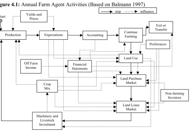
three major components: farms, markets, and land (Happe, Balmann, and Kellermann 2004) (see

figure 3.1). The use of AbM is appealing because each individual farm can be endowed with

specific characteristics and resource endowments. In addition, heterogeneous and spatial

characteristics of land can be included, meaning markets can be modeled using agents that

coordinate market activity (Happe, Balmann, and Kellermann 2004).

Figure 3.1:

Conceptual Model of an agricultural system (Adapted from Happe, Balmann, and

Kellermann 2004)

3.1 NetLogo

Platform

NetLogo

is a freeware platform suitable for modeling complex systems that develop over time

(Wilensky 1999). It is quite likely the most widely used platform for AbM research (Railsback,

Lytinen, and Jackson 2006). NetLogo

is continuously upgraded by the Center for Connected

Learning and Computer Based Modeling at Northwestern University, Evanston Illinois.

Within the NetLogo

platform, users provide rules to thousands of independent agents operating

concurrently, making it easier to analyze how micro level behaviour leads to macro level patterns

(Wilensky 1999). NetLogo

is fully programmable with the user creating the spatial

environment and the agents’ behavioral rules (Railsback, Lytinen, and Jackson 2006). NetLogo

has three classes of agents: turtles, patches, and observer (Wilensky 1999). Turtles are mobile

agents, which can move around the artificial world. Patches are fixed and represent the spatial or

geographic environment grid. The observer agent has no location, but has some control over

other agent classes. In this model, turtles represent the individual farming household located on

various patches of land. The observer represents the market auctioneer and coordinates land

markets.

3.2 Heterogeneity

In traditional economic models, homogeneity among agents is often assumed for simplicity and

mathematical tractability. A major strength of AbM’s are their ability to incorporate

Markets

Farm

farm 2

Land/

_Space

depends on influences

Enter Exit

heterogeneity in a relatively transparent manner. The agricultural region under study is

characterized by two main sources of heterogeneity: 1) individual agents and 2) land.

3.2.1 Agent Heterogeneity

There are three main agent types in this model: 1) farmers, 2) non-farming land owners, and 3)

the auctioneer, with the farmer being the most numerous. Farmers purchase and rent land used

for production activities while non-farming land owners hold land as an investment, and the

auctioneer coordinates the land markets.

Farming agents are endowed with different resources, abilities, and demographic characteristics.

Resources include capital, land, and labour. These are used for crop or livestock production by

farm agents in an attempt to generate income and wealth. Demographic characteristics include

age, education, and preferences. Although each agent has a common goal of maximizing wealth,

resource organization varies based on the individual’s preferences and resource endowment.

Agents also vary based on the risk aversion and preference for livestock production. In order to

increase wealth, the farm must expand by acquiring more land to increase production.

3.2.2 Land Heterogeneity

Land is arranged in plots of 640 acres and each plot consists of five categories of land: 1) tillable,

2) hay, 3) improved pasture, 4) natural pasture, and 5) waste. Tilled land can be used as pasture,

hay, or crop production. Hay land, consisting of natural hay, is unsuitable to be tilled and can be

used as either hay or pasture. Both improved pasture and natural pasture are used only as pasture

land and waste land is unsuitable for any use.

The area and quality of each category of land for each plot included in the simulation are based

on Saskatchewan Assessment and Management (SAMA) agency Data. Forage yields and land

value are based on SAMA quality, while annual crop yield indexes are also included for each plot

of land from Saskatchewan Crop Insurance Data.

1

_{Although it may be possible to improve land quality, it is likely very expensive. An example is the ability to haul}

in top good top soil, or remove water from a slough.

The spatial heterogeneity of land is captured through transportation costs for both hay and crop

production to the farmstead. Farm agent bid values for land will be directly affected by the

relative location of the plot in the land market.

3.3 Dynamics

Farm structure is largely influenced by a farmer’s ability to compete in farmland markets.

Farmland markets are the source of growth and represent change in land use when a new

individual gains control of additional farmland. The desire for farm growth causes farm agents to

compete in the farmland markets for the scarce immobile land resource. Farm operators in this

region are able to gain control of additional farmland through a primary farmland purchase

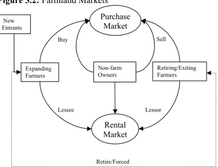
market and a secondary lease market (figure 3.2). Demand in the farmland purchase market is

created by farming operators hoping to expand and non-farming investors. Farmland is supplied

by exiting farmers and non-farming investors. The latter sell farmland when its return falls below

other investment opportunities. In the land lease market, demand is generated from farm

operators seeking to expand, but are unsuccessful, unable, or chose not to compete in the

farmland purchase market. Leased land is supplied by 1) retired farmers, who want to keep

control of their land, and 2) non-farming investors.

Figure 3.2:

Farmland Markets

Rental

Market

Purchase

Market

3.3.1 Farmer Bid Values in Land Markets and Land Use

Change over time largely stems from changes in control of land through the land market.

Changes in farm size along with farm numbers and a large portion of the transition of land use

occurs through a new individual gaining control of additional land and making the land use

decision. Farmers with sufficient capital and labour required to expand from one efficient point

to another, create bids based on their expected income from controlling the plot. Bid values are

therefore dependent on production costs, land use, and expectations, which determine how

competitive a farmer is in the farmland markets.

3.3.1.1 Cost of Production

In an environment where technology is constantly changing, machinery sizing is a major concern.

Varying cost structures are caused by the indivisible and lumpy nature of machinery and land.

Figure 3.3 demonstrates that as size increases the fixed costs of the investment are spread over

more units and decrease until an efficient point is reached. After the efficient size, diseconomies

are present due to farm operator’s inability to do work in a timely manner (or at all) with their

existing machinery. Past the efficient point, diseconomies set in and the per unit cost increases

until investment in more machinery allows the shift to AC 2.

Figure 3.3:

Average Cost of Production with Lumpy Investments

Accordingly, farms will jump from efficient point to efficient point as they expand their farm

operations. The fixed plot size of farmland does not allow farm operators to expand from an

efficient point without investing in more machinery and shifting to a new cost curve. The result

$/Acre

Acres

AC 1 AC 2

X