ADDRESSING PRACTICAL ISSUES IN DESIGNING WEATHER INSURANCE CONTRACTS FOR RISK MANAGEMENT APPLICATIONS IN DEVELOPING
COUNTRIES
A Dissertation by
LEONARDO FRANCISCO SÁNCHEZ-ARAGÓN
Submitted to the Office of Graduate and Professional Studies of Texas A&M University
in partial fulfillment of the requirements for the degree of DOCTOR OF PHILOSOPHY
Chair of Committee, Dmitry Vedenov Committee Members, David Bessler
Qi Li
Mark Welch
Head of Department, Parr Rosson
May 2014
Major Subject: Agricultural Economics Copyright 2014 Leonardo Francisco Sánchez-Aragón
ii ABSTRACT
In this dissertation we address practical issues in designing weather insurance contracts for risk management in developing countries in three different scenarios. First, we develop an innovative contract design strategy based on agronomic considerations that can be implemented in situations where only short and/or aggregate data series are available. We attempt to mitigate both the aggregate nature of yield data and the need for data-demanding analysis by looking at areas sharing the same growing conditions and using agronomic requirements to specify contract parameters. We find that the proposed contracts do not achieve the same degree of risk reduction as the contracts that can be constructed using no data limitations, but they do provide meaningful risk protection and typically at lower premiums. The implication is that the proposed methodology can be used to design weather derivatives for developing countries, where paucity of data often renders the conventional design approaches unworkable.
The second essay aims to derive a general-form optimal payoff of an index contract that takes into account potentially nonlinear dependence between the index underlying the contract and the loss that is insured. We find that the quasi-linear contract payoff structure may not be the optimal choice if the dependence between the index and the yield/revenue is nonlinear. The implication is that the proposed methodology can help to improve risk-reducing capabilities of weather derivatives particularly in situations where the effect of weather on yield is complex and not obvious.
iii
The third essay analyzes the use of weather derivatives in managing water supply risk arising in making water allocation decisions. The specific application is developed for the Alto Rio Lerma Irrigation District (ARLID) in the state of Guanajuato in Mexico. We argue that incorporation of weather derivatives in water allocation decisions can improve overall well-being of producers and allow shift water allocations from the wet to the dry season with the assumption that the wet season farmers can cope with the risk of water shortages by using weather derivatives. We find that use of weather derivatives does lead to better water allocation policies that allow the representative farmer to reach higher levels of utility. The implication is that introduction of weather derivatives can help to improve water management decisions in developing countries where agriculture heavily depends on irrigation and can be severely affected by extreme weather events.
iv DEDICATION
To my wife, Rosanna Huayamave, for giving me her beautiful smile during the darkness and her peace during the light.
v
ACKNOWLEDGEMENTS
I would like to thank my mother, who made the best of me and has taken care of my favorite’s guys, my pets Felino, Puschys, Snoopy, Lucas, Pochaco, Mateo y Mechas. I would like also to thank my parents-in-law who are always supporting me and
encouraging me with their best wishes.
I would like to express my deepest gratitude to my advisor, Dr. Dmitry Vedenov, for his excellent guidance, caring, patience, and providing me with an excellent
atmosphere for doing research. This dissertation could not have been finished without his help and support.
I would like to thank my dissertation committee members Drs. David Bessler, Qi Li and Mark Welch for all of their guidance through this process.
I would like to acknowledge the financial, academic and technical support of the Department of Agricultural Economics at Texas A&M University and its staff,
particularly Dr. David Leatham, the Associate Department Head for Graduate Studies. I would like to acknowledge the financial support of the Escuela Superior Politécnica del Litoral and the Secretaría de Educación Superior, Ciencia, Tecnología e Innovación.
Thanks also go to my friends and colleagues and the department faculty and staff for making my time at Texas A&M University a great experience.
vi TABLE OF CONTENTS Page ABSTRACT ... ii DEDICATION ... iv ACKNOWLEDGEMENTS ... v TABLE OF CONTENTS ... vi
LIST OF FIGURES ... viii
LIST OF TABLES ... xi
1. INTRODUCTION ... 1
2. PRACTICAL APPROACHES TO DESIGNING WEATHER DERIVATIVES UNDER YIELD DATA LIMITATIONS ... 4
2.1 Literature Review ... 7
2.1.1 Risk Management in Developing Countries ... 7
2.1.2 Reinsurance and Securitization ... 8
2.1.3 Weather Insurance ... 10
2.1.4 Application of Weather Derivatives to Agricultural Risks ... 12
2.2 Modelling Approach ... 15
2.2.1 Overview of Soybeans Production ... 17
2.2.1.1 Phenology of the Soybean Plant ... 17
2.2.1.2 Soil Characteristics ... 19
2.2.1.3 Proposed Soil Classification ... 20
2.2.2 Contract Design and Analysis... 20
2.2.2.1 Measuring Risk Reduction ... 22
2.2.2.2 Estimation of Distributions ... 24
2.2.2.3 Efficiency Analysis ... 26
2.3 Application: Arkansas Soybean Production ... 27
2.3.1 Soil Structure ... 28 2.3.2 Weather Data ... 28 2.3.3 Yield Data ... 29 2.3.4 Simulation Parameters ... 30 2.4 Results ... 32 2.5 Conclusions ... 34
vii
3. OPTIMAL CONTRACT STRUCTURE FOR WEATHER DERIVATIVES ... 36
3.1 Literature Review ... 37
3.2 The Model ... 38
3.2.1 Optimality Conditions ... 42
3.2.2 Algorithm for Solving the Euler-Lagrange Equations ... 44
3.3 Application Procedure and Data ... 46
3.3.1 Estimation of Distributions ... 47
3.3.2 Initial Guess for Indemnities Function ... 48
3.3.3 Weather and Yield Data ... 49
3.4 Results ... 49
3.5 Conclusions ... 52
4. USING WEATHER DERIVATIVES IN WATER ALLOCATION DECISIONS: A CASE OF GUANAJUATO, MEXICO ... 53
4.1 Literature Review ... 55
4.2 Irrigation Districts in Mexico ... 58
4.2.1 The Alto Rio Lerma Irrigation District (ARLID) ... 59
4.2.2 The Allocation of Water for Irrigation ... 60
4.3 General Modeling Approach ... 61
4.3.1 Baseline Water Allocation Model ... 62
4.3.2 Incorporating Weather Derivatives ... 67
4.3.3 Numerical Solution of Bellman Equation ... 69
4.3.4 Dynamic Simulation Analysis ... 71
4.4 Data and Problem Parameterization ... 72
4.4.1 Utility Function ... 72
4.4.2 Yield Data ... 72
4.4.3 Rainfall Data ... 74
4.4.4 Parameterization ... 76
4.5 Results and Sensitivity Analysis ... 77
4.5.1 Water Allocation Strategies... 77
4.5.2 Sensitivity to Coverage Level ... 79
4.5.3 Sensitivity to Prices ... 79
4.5.4 Effect of the Relative Risk Aversion Parameter ... 80
4.5.5 Sensitivity to Distribution of Rainfall ... 80
4.6 Conclusions ... 82
REFERENCES ... 84
APPENDIX A: FIGURES ... 95
APPENDIX B: TABLES ... 136
viii
LIST OF FIGURES
Page Figure A-1 Suggested classification of soil types for soybean
production………...…... 95
Figure A-2. Payoff structure of the agronomic contract with different
cap factor ....……….. 96
Figure A-3 Payoff structure of the agronomic contract with different
scale factor ....……… 97
Figure A-4 Locations of counties selected for analysis and
corresponding weather stations in Arkansas state………... 98 Figure A-5 Joint probability distributions of rainfall and soybean
yields, Independence County………... 99 Figure A-6 Joint probability distributions of rainfall and soybean
yields, Jackson County………... 100 Figure A-7 Joint probability distributions of rainfall and soybean
yield, Crittenden County……….. 101
Figure A-8 Joint probability distributions of rainfall and soybean
yield, Phillips County………... 102 Figure A-9 Joint probability distributions of rainfall and soybean
yield, Saint Francis County……….. 103 Figure A-10 Joint probability distributions of rainfall and soybean
yield, Pulaski County………... 104
Figure A-11 Joint and marginal probability distributions for rainfall
and soybean yields, Phillips county, maturity stage……… 105 Figure A-12 Joint and marginal probability distributions for rainfall
and soybean yields, Saint Francis county, maturity stage... 106 Figure A-13 Joint and marginal probability distributions for rainfall
ix
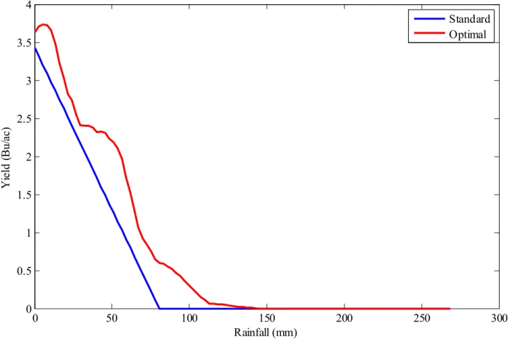
Figure A-14 Payoff structure of the standard and optimal contract,
Phillips county………. 108
Figure A-15 Payoff structure of the standard and optimal contract,
Saint Francis county……….……… 109
Figure A-16 Payoff structure of the standard and optimal contract,
Pulaski county……….…... 110
Figure A-17 The profit functions π of the wet-season farmers with and
without weather derivatives………. 111 Figure A-18 Payoff structure of the weather derivatives contract……... 112 Figure A-19 Barley (dry season) yields in module Valle de Santiago,
Mexico, 1989-2010……….. 113
Figure A-20 Sorghum (wet season) yields in module Valle de Santiago,
Mexico, 1989-2005……….. 114
Figure A-21 Relative frequency distribution of cumulative rainfall (from April to June) in the municipality of Valle de
Santiago, Mexico, 1942-2010………... 115 Figure A-22 Relative frequency distribution of cumulative rainfall
(from November to October, next year) at the dam Solis,
Mexico, 1961-2011………... 116
Figure A-23 Optimal water allocation policy without insurance………. 117 Figure A-24 Optimal state path without insurance………... 118 Figure A-25 Steady state distribution without insurance………. 119 Figure A-26 Optimal water allocation policy with insurance………….. 120 Figure A-27 Optimal state path with insurance……… 121 Figure A-28 Steady state distribution of water level in the reservoir
with insurance……….. 122
x
Figure A-30 Optimal water allocation policy with insurance for
different coverage levels……….. 124 Figure A-31 Optimal value function for different coverage levels…….. 125 Figure A-32 Water allocation decisions under different ratios of wet-
and dry-season crop prices without weather derivatives…. 126 Figure A-33 Water allocation decisions under different ratios of wet-
and dry-season crop prices with weather derivatives…….. 127 Figure A-34 Value functions for different ratios of wet- and dry-season
crop prices……… 128
Figure A-35 Water allocation decisions under different relative risk
aversion parameter without weather derivatives………….. 129 Figure A-36 Water allocation decisions under different relative risk
aversion parameter with weather derivatives………... 130 Figure A-37 Value functions for different relative risk aversion
parameter……….. 131
Figure A-38 Comparison of gamma probability distributions with
different shape parameters α………... 132 Figure A-39 Water allocation decision without weather derivative
when the shape parameter of the rainfall distribution for
Valle and Solis decreases 50%... 133 Figure A-40 Water allocation decision with weather derivative when
the shape parameter of the rainfall distribution for Valle
and Solis decreases 50%... 134 Figure A-41 Value functions when the shape parameter of the
xi
LIST OF TABLES
Page Table B-1 Water requirements and duration of each stage of soybean
growth……….. 136
Table B-2 Distribution of soil type across counties selected for
analysis………..…………... 137
Table B-3 Descriptive statistics of precipitation and temperatures for
single soil-type counties………... 138 Table B-4 Descriptive statistics of precipitation and temperatures for
mixed-soil counties……….. 139
Table B-5 Descriptive statistics of soybean yields for selected
counties……….……... 140
Table B-6 Estimated yield trend models………... 141 Table B-7 Estimated rainfall-yield models………... 142 Table B-8 Parameter of the best agronomic contracts for single
soil-type counties……….……... 143
Table B-9 Parameter of the best agronomic contracts for mixed-soil
counties……….……... 144
Table B-10 Parameters of the “optimal” contracts based on
econometric models………..…………... 145 Table B-11 Counties selected for analysis in Essay 2 with their soil
types and phenological growth stages……….. 146 Table B-12 Descriptive statistics of precipitation (in millimeters) for
selected counties………... 147 Table B-13 Descriptive statistics of soybean yields for selected
counties……….………... 148
xii
Table B-15 Parameter of the standard contracts for selected counties... 150 Table B-16 Comparison of the “standard” and optimal contracts for
the selected counties……… 151
Table B-17 Descriptive statistics of crop yields and water allocation in
module Valle……… 152
Table B-18 Trend models for barley (dry season) and sorghum (wet
season)………... 153
Table B-19 Descriptive statistics of precipitation at module Valle and
dam Solis………... 154
Table B-20 Parameters used in the dynamic model of water
1
1. INTRODUCTION
Adverse selection and moral hazard has been cited as the main reasons of failure of private crop insurance markets. As a result, insurers may not be able to provide any type of crop insurance in developing countries where the problem is compounded by the fact that the insurance markets may be incomplete or missing due to poor contract enforcement mechanisms and government inability to support crop insurance programs.
In the last years, there has been extensive research on the advantages of weather derivatives relative to traditional crop insurance (Skees and Barnett 1999); however, demand for these weather instruments has been lower than expected. While partly attributable to lack of familiarity with the products, the problem can be also traced back to the issues of contract design (Skees and Barnett 2006; Skees 2008; Miranda and Farrin 2012). This dissertation deals with practical issues arising in designing weather derivatives for risk management in developing countries in three essays.
The first essay attempts to deal with the yield data limitations by introducing a semi-naïve contract structure based on agronomic considerations and identification of homogeneous production regions. The approach is much less data-intensive than the design methods previously used in the literature and can be implemented in situations where only short and/or aggregate data series are available. In particular, we look at production areas sharing the same soil conditions rather than just the ones encompassed by arbitrary administrative boundaries. We use a simple index (one weather variable) and determine the parameters of the contract by using agronomical considerations. In
2
order to evaluate the effectiveness of this simple semi-naïve approach to index
construction, we use Arkansas soybeans as a test case. The extensive historical yield data available for this crop and region allows us to compare the performance of both the conventional contract designs and the ones developed in the essay. Given the similarities between growing conditions in Arkansas and South America, it is expected that the results would transfer to the case of soybean production in that region as well.
The research objective of the second essay is to derive an optimal form of payoff of an index contract that takes into account potentially nonlinear dependence between the index underlying the contract and the loss that is insured using the contract. Most of the existing papers on weather derivatives use a “standard” piecewise-linear contract to define the payoffs structure of the analyzed contracts. However, these contract payoff structures may not be the optimal choice if the dependence between the index and the yield/revenue is nonlinear. This framework is illustrated using weather insurance
contracts for Arkansas soybean as a case study. The results are then compared with those obtained in the first essay.
In the third essay, we look at potential improvements in water allocation
strategies that could be achieved by using weather derivatives. In many Latin American countries, the changes in temperature and shifts in precipitation patterns could affect the water supply, thus making the water allocation a major problem for agriculture.
A particularly interesting situation arises when there are two growing seasons, each characterized by different rainfall patterns but both dependent on irrigation. Weather derivatives can then incentivize adoption of allocation patterns that shift water
3
allocations to the dry season from the wet season with the assumption that the wet season farmers can cope with the risk of water shortages by using weather derivatives. These financial instruments might also induce an inter-temporal reallocation of water in irrigation districts, increasing the efficiency of water use in the long term. The essay applies the analytical model to the Alto Rio Lerma Irrigation District in the state of Guanajuato in Mexico.
4
2. PRACTICAL APPROACHES TO DESIGNING WEATHER DERIVATIVES UNDER YIELD DATA LIMITATIONS
In the last 10 years, methodological advances in designing weather-based
insurance instruments have increased expectations for their performance, mainly in rural areas of developing countries (World Bank 2005; Hazell et al. 2010). Pilot programs have been developed for Mexico, India, Malawi, China, Nicaragua, India, Morocco, among others. For the exception of Mexico and India, demand for these weather instruments have been lower than expected (Hess 2003; Barnett and Mahul 2007; Giné and Yang 2009; Giné et al. 2010)1.
Factors like the lack of appropriate formal insurance markets, the absence of institutional framework to support trading between international and local institutions, potential basis risk, no consensus between farmers and insurers on which weather variables affect yields, and the lack of agreement over a common pricing model are the most typical explanations for that behavior given in the literature (Dischel 2002;
Richards et al. 2004). In this context, basis risk emerges as the prevalent contract design
problem, which affects the reliability of protection that index insurance contract may offer to small famers (Miranda 1991; Doherty and Richter 2002; Cummins et al. 2004; Barnett and Mahul 2007).
1 Depending on the context, weather-based insurance instruments can be treated either as insurance contracts or as options written on realization of the index. However, there is no difference between these two frameworks from the standpoint of contract design and risk-reducing efficiency. For the rest of this essay the weather-based risk management instruments will be referred to as weather derivatives or index insurance contracts interchangeably.
5
Basis risk arises when a policyholder receives an indemnity payment that does not match the actual loss (Varangis et al. 2003). The aggregate nature of yield data, complex relationship between weather measurements and actual loss, and spatial variability of weather conditions are the most commonly cited sources of basis risk (Manfredo and Richards 2005). This risk can be reduced through product design (Skees 2008), with several approaches available. The existing literature primarily concentrates on finding the most accurate relationship between weather and losses. Other approaches consider limiting index insurance to low-frequency, high-impact events such as
hurricanes or extreme droughts. It is thought that, under such extreme conditions, farmers’ losses may be better correlated to the underlying weather variable.
Basis risk can be magnified even more in developing countries where data are often limited and unreliable. In such situations, insurance companies use aggregate data to develop insurance products whose payments are contingent upon indices presumably correlated with individual loss (Goodwin and Mahul 2004). The shortness of data series also contributes to the basis risk, since the available data is insufficient for establishing weather-loss relationship using the conventional econometric methods.
The design methodology presented in this essay attempts to circumvent the limitations of available yield data and reduce the basis risk inherent in the contracts. First, the contracts are designed for homogeneous production areas with the expectation that yield variability in the area is comparable to that on a single farm. In this case, the available aggregate yield data can be considered as more accurately representing the distribution of yields of individual farms in the area. In particular, we look at production
6
areas sharing the same soil conditions rather than just the ones encompassed by arbitrary administrative boundaries. Furthermore, instead of constructing the indexes based on econometric models, we use a simple index (one weather variable) and determine the parameters of the contract based on agronomic considerations.
The research objective is not to develop a new or better way of constructing index insurance contracts, but rather to evaluate the effectiveness of a simple semi-naïve approach to index construction that can be implemented in situations where only short and/or aggregate data series are available. While the potential of this approach can be mostly appreciated in developing countries, we use Arkansas soybeans as a test case. On the one hand, long and reliable data series are available for this crop and location, which allow us to validate this approach. On the other hand, there are similarities between soybean productions in Arkansas and Latin America, which would allow us to transfer the results to that region.
The rest of the chapter is organized as follows. Literature on index insurance contracts is reviewed first, with particular attention to various design procedures. We then briefly explain the growth process of soybean plants, identify environmental conditions required for optimal growth, and determine soil types best suited for soybean production. The second subsection presents the methodology used to design the
proposed weather derivative contracts and evaluate their effectiveness as a risk reduction tool. The third subsection describes characteristics of soybean production in Arkansas, data collection process, and identification of homogeneous production zones. The fourth
7
subsection presents and discusses the results. The final subsection concludes and discusses directions for future research.
2.1Literature Review
2.1.1 Risk Management in Developing Countries
Unfavorable weather conditions are one of the main risk factors affecting agricultural production and agri-business (Dercon 2002). These factors have a significant impact on farmers’ decisions related to production and investment, on their ability to service debts, and on their standards of living. Traditionally, farmers have utilized nonmarket
institutions2 such as family, local, or community lending institutions as informal risk transfer mechanisms in rural areas (Ellis 2000). Informal loans, diversification of income sources, and crop diversification have also been mechanisms used by rural household to smooth consumption (Morduch 1995; Fafchamps and Pender 1997; Zimmerman and Carter 2003). However, when an extreme weather event occurs, these nonmarket institutions fail as risk management tools because of their limited capacity to spread correlated risks affecting farmers in the same area at the same time (Skees et al. 1999).
The extreme weather events such as drought, floods and windstorms strangle rural household economy which owns few assets. Due to high risk exposure, rural household become more risk averse and adopt low risk investment strategies associated with low return, which is not enough to allow rural households to escape of the poverty trap (Carter and Barrett 2006).
8
Insurance companies are often reluctant to conduct business in rural areas due to poor contract enforcement mechanisms. Because of the asymmetric information
problems, insurance companies have to invest in monitoring mechanisms, require tradable collaterals, and impose high deductibles and co-payments (Hess et al. 2002). Since losses are spatially correlated across farmers, an extreme event could increase the number of defaults among farmers which in turn would represent additional liquidity problems (Skees and Barnett 2006; Skees et al. 2007). All these factors increase premiums and thus reduce demand for crop insurance.
Countries respond to weather-related risks by taking action both before and after the extreme weather events. As ex-ante strategy, governments have supported a variety of crop insurance programs. All of these have relied on government subsidies and yielded mixed results (Goodwin and Smith 1995). As ex-post strategy, governments often redirect resources used usually in activities such as education or health to cover damage caused by natural disaster. Because of these programs, farmers would not internalize the costs of weather risks and would be more dependable on public relief (Skees et al. 1999). In general, both governments and rural household of developing countries have not been effective in managing risk transfer neither ex-ante nor ex-post of a shock (Hazell 1992; Barnett et al. 2008).
2.1.2 Reinsurance and Securitization
Weather insurance was first conceived for the purposes of reinsurance of systemic risks. Extreme weather risks represent an enormous financial problem for the insurance companies because thousands of claims have to be paid within a relatively
9
short period. In order to deal with these losses, insurance companies traditionally looked to unload weather risk using reinsurance as an ex-ante funding source. It allowed the insurer to raise its capital in the aftermath of the natural disasters by hedging its risk exposure with reinsurance companies which, in turn, diversified their portfolios by taking risks in other regions.
In spite of the advantage of reinsurance, insurance companies could not always transfer their risk exposure to reinsurers. Froot (2007) gave several explanations for this result, such as lack of reinsurance supply, market power of reinsurers, the price of the reinsurance contracts, and asymmetric information between insurer and reinsurer3.
Securitization could be a natural way to introduce market efficiency and to provide an affordable insurance for weather-related risks. Securitization pools certain types of assets and repackage those into interest-bearing securities (Simmons 2003). In case of weather risks, these were tied to a specific weather event and were divisible so as to allow an investor to buy any amount of risk exposure.
The literature on catastrophe securities provides a number of arguments in favor of this approach (Lewis and Davis 1998). In particular, insurance companies could get sufficient capital to cover their exposure to catastrophe risk from the financial market. Since weather risks are not related to the performance of capital markets, insurers could get cheaper source of funds.
10 2.1.3 Weather Insurance
Weather insurance contracts were proposed in the literature as a natural extension of weather-linked reinsurance arrangements to primary insurance markets, in particular to deal with risks of agricultural production (Miranda 1991; Miranda and Vedenov 2001; Hess et al. 2002).
These insurance contracts are typically modeled as options whose payoffs are linked to realizations of specific weather variables such as number of heating or cooling degree days, rainfall level, etc. Most of the literature structures these contracts as a put (call) option with payoff triggered by a specific weather variable falling below (rising above) a pre-specified level. These payoffs can also be triggered by realizations of an index, which correlates losses and weather. The latter can be constructed based on an econometric relationship between weather and yield (Martin et al. 2001; Turvey 2001; Vedenov and Barnett 2004).
The key advantages of these insurance contracts over the traditional insurance products usually mentioned in the literature are as follows (Miranda and Vedenov 2001; Barnett and Mahul 2007):
The contract structure is simpler than that of traditional insurance.
The weather variables or indices are measured objectively and transparently and do not depend on actions of either farmers or insurers. Neither farmers nor insurers have better information about the future realization of the index or the dependence relationship between losses and the index.
11
Operating costs are low due to lack of asymmetric information or moral hazard. The major disadvantage of index insurance is the so-called basis risk. It arises when farmers’ losses are poorly correlated to the index used in designing a weather-based contract. In this case, a farmer could receive an indemnity payment that does not match the actual loss (Varangis et al. 2003).
There are three potential sources of basis risk. First, specific relationship between weather and yields is rather complex and not fully understood. Most of the approaches to designing indexes are based on econometric estimation of weather-yield relationship function which is then used as an index (Martin et al. 2001; Turvey 2001; Vedenov and Barnett 2004). This method, however, requires adequate data series, which may be a problem in developing countries.
The second potential source of basis risk is the yield data used for such
estimations is typically aggregated over a larger production area (e.g. a county), which could also affect the performance of the insurance contracts. Ideally, farmers would prefer contracts written on a weather index designed for their individual farms, but farm-level data are rarely available especially in developing countries. Contracts based on weather measured at a specific farm maybe less attractive to outside investors and would affect the possibility of risk transfer to capital markets. These insurance contracts are often designed based on more easily available area yields. The downside of this approach is that the variability of aggregate yields is typically lower than those of individual farmers.
12
Third, the spatial variability of weather conditions affects the reliability of weather contracts. Given that the underlying weather variables are measured at specific locations, the impact of this measure can be diluted as one moves away from the weather station (Manfredo and Richards 2005).
All these problems can hurt the performance of the weather insurance product; however, the basis risk can be reduced through product design (Skees 2008).
2.1.4 Application of Weather Derivatives to Agricultural Risks
Turvey (2001) examined if weather derivatives could provide a hedge against production risk in Ontario. The relationship between crop productivity and weather events was estimated assuming a 2-input production function (rain and degree-day heat). The quadratic and Cobb-Douglas production functions were considered, although the goodness of fit was low. Given that no other specifications were explored and the limited evidence provided for these function, contract parameters based on this estimations could be inconsistent. The author’s approach relies on daily data, which could be a challenge to obtain in developing countries. In addition, the author also assumed that farmers know what weather events to be insured against because he allowed farmers to choose contract parameters.
His concluded that farmers could reduce risk exposure to weather events purchasing these instruments. His models however, did not consider specifics of crop growth which could affect the performance of the weather derivatives. The author pointed out the need to minimize basis risk.
13
Martin et al. (2001) considered European put options on precipitation. These contracts start paying when the index falls below a specified strike. Once the index falls below a limit, the payoff “maxes out” at the maximum indemnity level. When the index falls between the strike and the limit, the contract pays a proportion of the maximum indemnity. This type of contract is completely designed once the values of strike, limit and maximum indemnity are specified. The authors used cumulative daily precipitation for September and October in Stoneville, Greenville and Cleveland counties in
Mississippi as the index. Farmers were allowed to choose the parameters of the contract according to their risk management needs. Using extended time series of weather data, the authors estimated expected loss cost from the simulated historical loss costs. They used a gamma distribution to model cumulative precipitation. Their results encourage the use of weather derivatives within the US agriculture.
Vedenov and Barnett (2004) evaluated the efficiency of weather derivatives constructed as put or call options. Similar to Martin et al., these contracts start paying when the index falls below/exceeds a specified strike ∗. Once the index falls below/exceeds a limit ∗, the insured receives the maximum indemnity . When the index falls between the strike and the limit, the contract pays a proportion of the maximum indemnity. A formal payoff schedule for the put option can be written as
14 (2.1) | , ∗, 0 ∗, ∗ ∗ 1 ∗ ∗, 1 ∗,
where the parameter varies between 0 and 1, with the limiting case of 0 corresponding to the conventional proportional payoff with deductible, and 1 corresponding to a “lump-sum” payment once the contract is triggered regardless of the severity of the shortfall. The payoff for the call option can be written in a similar way with obvious changes.
The authors used district level yield data for corn, soybeans, and cotton in major respective production areas in the U.S. in order to construct weather indexes. They found that constructed weather derivatives may provide risk reduction for the considered crop/district combinations. Though they estimated models with complex combinations of weather variables, they obtained relatively low goodness of fit (36% at most). They used an ad hoc selection of weather variables (e.g. monthly average temperatures and cumulative monthly rainfalls) The weather derivatives were designed for relatively large geographic areas in order to avoid problems such as weather data availability and allow for risk transfer to capital markets, but this came at a cost of added basis risk.
Since the late 1990s, a number of studies considered implementation of index insurance for agriculture in developing countries (Hazell 1992; Miranda and Vedenov 2001; World Bank 2005). The majority of these papers relied on availability of extended series of weather and crop yield data, which is often not the case in developing countries. For instance, Skees et al. (1999) examined the performance of rainfall insurance in
15
Nicaragua, which is affected by insufficient or excess rainfall. In order to ensure the sustainability of such an insurance scheme, they recommended the development of extensive crop yield data sets to design and price the insurance.
Linear dependency between crop yield and the index has been usually assumed in literature (Skees et al. 2001; Turvey 2001; Hess 2003; Deng et al. 2008). These approaches may reduce the effectiveness of index insurance contracts, since they only rely on the strong monotonic dependence between crop yield and the index rather than a linear dependence.
Except for Vedenov and Barnett (2004), the authors typically assume that farmers have a complete knowledge about what type of weather instrument satisfy their requirements. Finally, there is no information on specifics of plant growth incorporated in the design of weather contracts.
2.2Modelling Approach
We assume that we are presented with a short yield data series (20 years or less) averaged over an area such as a county or a comparable administrative unit. We propose to mitigate the problems with data by designing weather insurance contracts in the following way.
First, based on agronomic criteria such as soil pH, soil texture and drainage, we identify the composite types of soils best suited for the production of crop under investigation. Then, we use the developed classification to detect homogeneous production areas among the administrative units for which we have data. Specifically, we try to identify counties with a single or a predominant soil type. We expect that the
16
variability of yield aggregated over these areas is comparable to that of any given farm within the area. We perform the analysis looking at areas sharing the same soil
conditions rather than just the ones encompassed by arbitrary administrative boundaries. Second, we select indexes based on growing requirements for the crop during each phenological stage and for the entire growth season.
Third, we determine the parameters of the contract by using agronomical considerations, viz. the minimum and maximum requirements of the weather variable chosen as an index.
In order to illustrate the proposed methodology, we apply it to the design of weather derivatives to Arkansas soybeans.4 In particular, we use rainfall as an index and construct cumulative daily rainfall variables for each stage of soybean growth and the entire crop season. We consider both the excess and lack of water to be equally detrimental. Therefore, the designed contract is set to trigger when the rainfall falls outside of the optimal range suggest by agronomist. We call the proposed contract the agronomic contracts.
In order to evaluate the effectiveness of the agronomic contract, we compare it with the contracts designed according to the methodology proposed by Vedenov and Barnett (2004).
4 As pointed earlier, while this case does not represent the situation with data we are trying to address, availability of long data series allows us to evaluate the performance of the proposed contracts against the benchmarks established in the literature.
17 2.2.1 Overview of Soybeans Production
The most comprehensive reference on soybean production is published by The Center for Agricultural Bioscience International (Singh 2010). The latter describes factors affecting soybean growing —geography, climate, land and soil. Other
comprehensive sources include Heatherly and Hodges (1999) and Arkansas Soybean Handbook which describe phenological growth stages of soybeans and how various aspects such as soil texture affect soybean production. A comprehensive manual on crop water needs is written by Brouwer and Heibloem (1986). The remainder of this section presents summary of relevant information contained in these sources.
2.2.1.1Phenology of the Soybean Plant
Soybeans are classified as a short-day plant, because the duration of darkness regulates the flowering. The cumulative water requirement from planting to harvest is between 450 and 700 mm, with daily consumption that varies as the crop develops. Soybean production requires good drainage as standing water can increase the incidence of diseases. Well-planned drainage provides better soil aeration, higher soil
temperatures, better impact of herbicides, better soil structure and higher yields. Poor drainage increases the chance of plant diseases and insects/pests because herbicides cannot reach the soybean root zone.
Soybean plant develops over three distinct sequential stages (vegetative, reproductive and mature) that influence each of the three yield components —the number of pods per plant, the number of seeds per pod and seed size.
18
The vegetative stage begins when seed are exposure to moisture and soil temperature of 55 to 60F. Usually in the first 15 days after planting, the cotyledon emerges above the soil surface and nodes appear on the main stem with fully developed leaves during the next 36 days. The water demand is around 15-26% of the total water requirement and needs to be applied at uniform rates during the 51-day period. Short-term excess water during the early vegetative stages can cause yield reductions depending on soil texture.
The reproductive stage begins when a soybean plants blossom and lasts until pods and leaves are developed. The process takes about 64 days to complete, during which seeds reach their full size. The water need at this stage is around 55-64% of the total water requirement. Water stress reduces number of pods per plant and affects grain-filling.
The maturity stage begins when pods on the main steam have reached their mature color and lasts 18 days. During this time, dry weather is required to reduce the moisture content in soybeans. The water need on this stage is approximately 10-20% of the total water requirement. At this stage, drain decisions may be critical. Early drainage speeds up the harvest but can negatively impact the grain filling, which in turns, affect the soybean weight.
The growth of soybean plants can also be negatively affected by critical temperatures (below 55F and above 95F) across different growth stages. Table B-1 summarizes the water requirement and the duration of each stage.
19 2.2.1.2Soil Characteristics
Soybean productivity also depends greatly on soil characteristics. Soil texture determines the amount of water available to plants, how well-aerated the soils are, and the rate at which water moves to roots. Based on the proportion of various particle sizes present in soils, their texture is classified as fine, medium, or coarse. Fine-textured soils are dominated by tiny clay particles, while coarse-textured are characterized by larger-size sand particles. Medium-textured soils contain various proportions of clay, sand and silt. Coarse-textured soils such as loamy sand and silt loam are better suited for soybean growing than clay and medium-textured soils because the former maintains
well-balanced nutrient levels, reduces erosion, moves air and water to the roots and supports rapid growth.
Soybean plants also require a right balance of acidity for high quality yield and healthy crops. The soil pH is a measure of acidity or alkalinity in soils and affects the ability of soil organisms to survive, which in turn transform organic matter into plant nutrients. Soybean can grow in soils with a wide range of pH, from 5.8 (slightly acid) to 7 (neutral). Soils with pH above 7 are considered marginal and not suitable for soybean production. High pH levels are detrimental for soybeans, because nutrients such as phosphorus, calcium and nitrogen are unavailable in such soils. Yields are also negatively affected when soil becomes too acidic (low pH), although this can be mitigated by adding liming materials before fertilizing.
20 2.2.1.3Proposed Soil Classification
Based on the information above, we attempt to identify the composite types of soils best suited for soybean production.
We designate the optimally suited soil as Soil Type I. The latter is characterized by coarse texture, pH level 5.8 to 7 and good drainage. As mentioned above, coarse-textured soils are more fertile than fine-coarse-textured because the former has a relatively high amount of water available to plants. Also, coarse-textured soils do not require much attention because they can maintain a steady pH level so that farmers would not need to reduce soil acidity. The pH level between 5.8 and 7 guarantees the availability of soil nutrients to plants and avoid damage to rotational crops. These characteristics together with good drainage enable soybean cultivation.
Fine texture soils regardless of pH level and soil drainage are designated Soil Type III because it is the least suitable type for soybean production. Fine-textured soils have small amount of water available to plants because of their small-sized particles. Large economic losses can occur when soybeans are cultivated on fine-textures soils because of the Phytophthora diseases.
All other combinations of soil characteristics are grouped as Soil Type II. The latter combine coarse and medium texture and pH level less than 7 regardless of soil drainage. The properties of all constructed soil types are summarized in figure A-1. 2.2.2 Contract Design and Analysis
We follow the general contract design approach of Martin et al. (2001) and Vedenov and Barnett (2004), with necessary modifications to accommodate out
21
modeling strategy discussed above. In particular, cumulative rainfall over a specific phenological stage is used as an index. The contract is set to trigger only when the rainfall falls outside of the optimal range since both the excess and lack of water can be equally detrimental to plan growth. In other words, the contract has two triggers
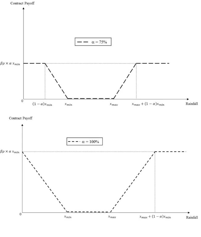
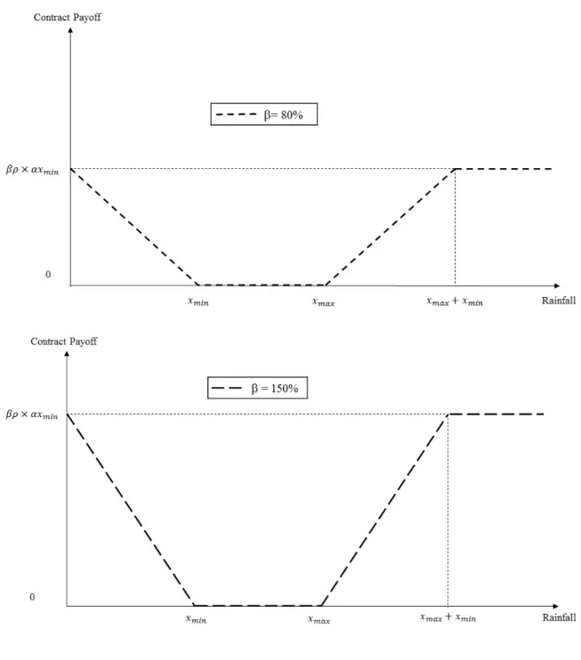
suggested by agronomic criteria. Formally, the contract indemnity (expressed in units of yield) can be presented as:
(2.2) | , , , , 1 1 0 1 1
where is the cumulative rainfall level over a specific period, the trigger points and correspond to the minimum and maximum water requirement during the period based on agronomic recommendations, is a conversion factor between the units of rainfall and units of yield5. The parameter 1 is used to cap the contract payoff for
5 We define this as the ratio of average crop yield and average cumulative rainfall during the entire crop season.
22
tractability purposes.6 Since index contracts are subject to basis risk, the buyer is also allowed to increase or decrease the amount of insurance protection by the scale factor , similar to the Group Risk Plan (GRP) offered in the U.S. (Deng et al. 2007). The scale factor adjusts the indemnities so that those could better track actual losses. The
indemnity schedule (2.2) is illustrated in figures A-2 and A-3.
Figure A-2 shows payoffs of two contracts with the scale factor of 100 percent and the cap factors of 80 and 150 percent. Figure A-3, shows two contracts with the cap factor of 100 percent and scale factors of 75 and 100 percent.
2.2.2.1Measuring Risk Reduction
The effectiveness of the designed contracts in reducing risk is measured within the expected utility framework. The analysis is performed from the standpoint of an economic agent who is not necessarily directly involved with the production, but is involved with the economic activity directly affected by the agricultural production risks (i.e. a “risk aggregator”). For example, county cooperatives that give loans to farmers are directly affected by the farmers’ losses because the latter affect the probability of
payoffs. The rationale behind this approach is that the index insurance contract protect better against systemic risks rather than idiosyncratic risks of individual producers. A portfolio of risks aggregated over a properly defined area would diversify away such
6 For the tractability of this contract, its payoff must be at least constrained on the excess side where it can be potentially infinite. Since the payoff is naturally limited on the deficiency side (at 0), this provides for a convenient overall cap which corresponds to 1. Values of 1 are considered to allow for a possibility of a cap set at a fraction of the maximum payoff on the deficiency side. The latter is similar to the maximum payoff constraint parameter utilized in Vedenov and Barnett (2004).
23
idiosyncratic risks, but would still be exposed to the area-wide risks typically associated with the extreme weather events (e.g. droughts, floods, hurricanes, etc.).
We assume that there is one such "risk aggregator” in a given county/region, that aggregator’s choice of insurance is driven by expected utility maximization motives, and that its preferences over risky alternatives can be represented by a utility function ∙ 7
defined over the total revenues expressed in units of yield.8
If no insurance is available, the aggregator utility is simply
(2.3)
where is crop yield, and the expectation is taken over its distribution. If we assume that a random variable (weather index) can communicate information about (crop yield), and an insurance contracts on is available, then the utility becomes
(2.4)
where the indemnity function is as in equation (2.2), is the contract premium9, and the expectation is taken over the joint distribution of the index and yield .
7 This aggregator derives utility from the county-level yield, but the nature of that utility depends on the nature of the aggregator. For purpose of this analysis, we do not specify the latter.
8 This assumption can be relaxed in a trivial way if prices are fixed and nonrandom. Stochastic prices can be accommodated within the same framework, although practical application would require additional historical price data, which may or may not be available.
24
Without loss of generality, we assume that the premium is actuarially-fair and is equal to the expected payoff of the contract10, i.e.
(2.5) | , , ,
where all parameters are the same as in equation (2.2) and the expectation is taken over the distribution of the index .
Under these conditions the agent would decide to buy the insurance contract if the expected utility of revenue with the contract is greater than the expected utility without the contract. For illustrative purpose the expected utility can be conveniently represented by the certainty equivalent levels (Schnitkey et al. 2003), namely:
(2.6) ∙
The risk reduction due to the weather derivative can be then computed as Δ . The contract has a value to the aggregator and reduces its risk exposure if Δ 0.
2.2.2.2Estimation of Distributions
In order to compute premiums and certainty equivalent revenues in equations (2.5) and (2.6), the joint distribution of yield and rainfall , and the marginal distribution of rainfall are required.
25
A typical approach here is to assume a parametric functional form and then estimate the unknown parameter(s) based on historical data. Given the shortness of data series and the lack of valuable prior information about the underlying data generation process of yield and the index, parametric estimations can be unreliable.
The alternative is to use nonparametric methods, which impose fewer
assumptions and rely on data to determine the shape of the distributions. In particular, we use kernel-density method (Wand and Jones 1994) to estimate the marginal
distributions of rainfall and yield, viz.
(2.7) 1
where is the random variable of interest (either the index or the yield ), ∙ is a kernel function, is the degree of smoothness, and are the observations (historical realizations) of interest.
Following Charpentier et al. (2007), we estimate non-parametric copula density
(2.8) , 1 , , ,
where ∙ is a bivariate kernel function, and are the degrees of smoothness (Li and Racine 2011), and , is the empirical distribution functions defined as
26
(2.9) , 1
1
where the indicator function takes the value of one if the condition is satisfied and zero otherwise. The marginal distributions (2.7) and the copula estimator (2.8) are combined to construct the joint probability distribution using the Sklar’s theorem (Sklar 1959). The latter postulates that any joint distribution can be decomposed into its marginal distributions and a copula function which captures the dependence structure between variables, namely,
(2.10) , ,
2.2.2.3 Efficiency Analysis
In order to evaluate the effectiveness of the agronomic contract, we compare its risk-reducing capability with the benchmark contract designed according to the
methodology in Vedenov and Barnett (2004). In addition, we analyze variations of the agronomic contract constructed both for the entire season and for each stage. We also consider agronomic contracts written on the excess of water, the lack of water or both. All variations of the agronomic contracts and the Vedenov and Barnett (2004)’ contracts are constructed based on the same data set.
We express the risk reduction in terms of the certainty-equivalent payouts of these contracts. The goal is not to obtain the best contracts (by construction there are
27
not) but rather to see how close the performance of the optimal contracts can be approached by the agronomic contracts in the situations when one cannot rely on extended data series or when data aggregation may create potential problems. 2.3Application: Arkansas Soybean Production
Soybean production in Arkansas has characteristics similar to those found in South America, especially in Argentina, Brazil, Bolivia and Paraguay. Many producers plant soybean on marginal lands without irrigation, especially in the lower Mississippi River valley. The increasing value of water together with the reduced amount of inputs required make farmers increase the amount of acreage devoted to non-irrigated soybeans. Under these conditions, the effects of drought or flood could increase the variability in soybean production.
Arkansas, located about 35N of the equator, has temperatures influenced by the Mississippi River and the Ozark and Ouachita mountains. Argentina and Brazil, the biggest soybean producers in South America, have temperatures more stable than
Arkansas. Argentina soybeans are grown in temperate regions (35S of the equator) with rainfall during the growing season. Brazil, with soybeans regions closer to the equator, has a wetter climate and higher rainfall than Arkansas.
Arkansas soybean growers apply various production systems under different tillage regimes which may or may not include irrigation. Under non-irrigated system, farmers can stabilize yield from year to year when they combine high-yielding varieties with different maturity date (Ashlock, Mayhew, et al. 2000).
28 2.3.1 Soil Structure
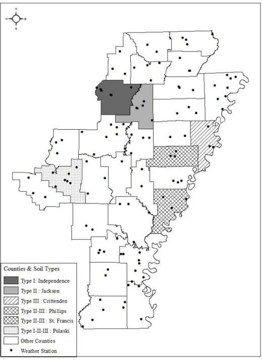
In order to apply the classification suggested in figure A-1, we combined the Arkansas maps of landforms, soil texture, pH level and soil drainage provided by Soil Survey Staff, et al. The resulted map was combined with the soybean area map provided by USDA/NASS Cropland Data Layer and USDA/SSURGO.
We identified counties that are composed mostly of a single soil type or
combination of at most two types. Six counties selected for analysis are listed in table B-2 along with the distribution of soil types in each.
Independence County mostly has Soil Type I (63.1 percent), while Jackson County is predominantly Soil Type II (78.6 percent). Crittenden mostly has soil type III (78.6 percent). Phillips and Saint Francis Counties have a mixed soil composition — a combination of soil types II and III. Finally, Pulaski County combines all identified soil types. Mixed soil type counties are included in the analysis in order to verify the
conjecture that agronomic contracts are more effective when constructed for areas with similar (homogeneous) growing conditions. Figure A-4 shows the location of selected counties.
2.3.2 Weather Data
Daily precipitation and temperature data recorded at the weather stations nearest to the selected counties were collected from the NOAA/NCDC. Locations of the weather stations are shown in figure A-4. The data were used to construct cumulative rainfall variables by stage and for the entire growing season. Since Arkansas farmers use different soybean varieties with different growing periods, it was impossible to
29
determine specific planting dates and stage durations for each individual producer or the county as a whole. Instead, we used average planting dates and average stage durations reported in Ashlock and Purcell (2000) (see table B-1).
Average temperatures by stage and for the entire season were generated in a similar fashion. Tables B-3 and B-4 show descriptive statistics of both cumulative rainfall and average temperature by stage, assuming June 15 as planting date (Ashlock, Klerk, et al. 2000). Data show that daily temperatures in selected counties do not fall outside of the agronomic requirement, for that reason temperature was excluded from our analysis. However, availability of rainfall is critical and it is the main constraint during the crop season.
2.3.3 Yield Data
Historical county-level yield data for non-irrigated soybean production in the selected counties for 1972-2012 were collected from USDA/NASS. The descriptive statistics of the yields are listed in table B-5. These selected counties accounted for 63.6 percent of Arkansas non-irrigated soybean production in 2012.
KPPS test, Dickey-Fuller and Phillip-Perron tests were performed to detect whether yields have stochastic trends. All these tests agree that yield series are trend stationary.11
New disease-resistant and high-yielding soybean varieties have been introduced in Arkansas over time. These improvements make soybean yields incomparable across years. To address this problem, yields series were detrended following Vedenov et al.
30
(2006). In particular, a piecewise log-linear trend equation was fitted for each yield series. The general form of the estimated equation is
(2.11) ln ⋯
where ln is the natural logarithm of yield in year ; , for 1, … , , represent the years at which the slope of the trend line changes, are dummy variables which are equal to 1 for all observations such that , and 0 otherwise and is the error term.
We used a nonlinear least square procedure to estimate model (2.11). This method allowed us to find the points that result in the best fitting model. Table B-6 shows the best fit models and their statistics for selected counties.
Based on these estimations, the detrended yields were then calculated as:
(2.12)
where is the trend predicted for year . 2.3.4 Simulation Parameters
Epanechnikov kernel was used to estimate both the marginal CDFs and PDFs for yield and rainfall. The same kernel was also used to estimate the copula function. The rule of thumb was used to estimate the bandwidth (Li and Racine 2011). CRRA power utility function
31
(2.13) ,
1
was used to reflect the preferences, with the risk aversion parameter ranging from 1 to 3 (as per Myers (1989) and Wang et al. (1998)).
The expected utilities in equations (2.3) and (2.4) were integrated numerically using Simpson’s quadrature method (Miranda and Fackler 2002) on a 501 501 grid over the ranges of yield and rainfall distributions. The trigger points and for each stage were set according to table B-1. The range of cap factor in equation (2.2) was set from 70 to 100 percent and the scale factor from 85 to 150 percent, both in 5% increments. The conversion factor was set equal to the ratio of average yield and average water needed in the entire season. The risk reduction of agronomic contract specified in equation (2.2) was evaluated for situations when the risk aggregator is allowed to purchase contracts on excess of rain, lack of rain or both.
The effectiveness of the agronomic contractswas compared with that of the contract designed according to Vedenov and Barnett (2004). The weather index was constructed using parametric regressions between soybean yield and cumulative precipitation for each growth stage. Table B-7 shows the “best fit” models and their statistics.
Indices estimated by these models were then used to calculate payoffs of the standard contracts in equation (2.1). The optimal values of the strike ∗, the limit and
32
the maximum indemnity were determined so as to maximize the expected utility with the contract. The risk reduction was calculated following equation (2.6).
2.4 Results
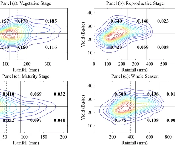
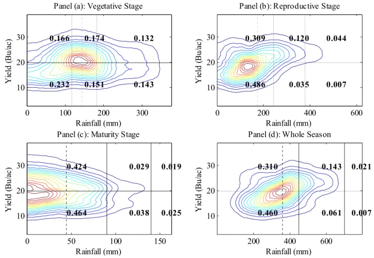
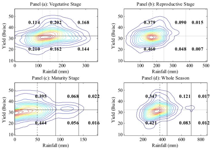
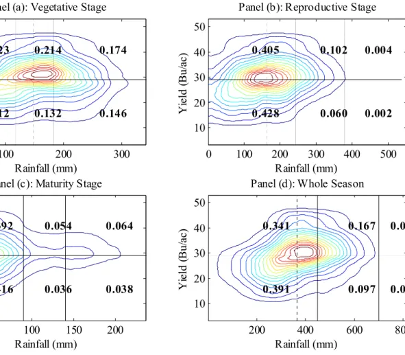
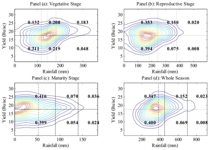
The risk-reducing effectiveness of agronomic contracts varies both across counties (or soil types) and stages. Figures A-5 through A-10 show the estimated joint distributions of soybean yield and rainfall for each growth stages for selected counties. The vertical lines indicate the minimum and maximum water requirements in each stage. The horizontal line represents the average soybean yield. Numbers in bold represent the joint probability of drawing a rain-yield from the respective ranges of rain and yield.
Unclear dependence between crop yield and rainfall were found for the vegetative stage regardless of soil types (except for Phillips and Pulaski Counties) suggesting a substantial amount of basis risk (see figures A-5 – A-10). This pattern continues in the maturity stage as well. However, there appears to be a more pronounced dependence between yields and rainfall in the reproductive stage. In particular, the probability of obtaining low yields when the rainfall is outside of the optimal range is higher at this stage than at any other. Finally, the joint distributions of yields and rainfall for the entire season exhibit a stronger dependence structure than the individual stages. Tables B-8 and B-9 summarize parameters and risk reduction effectiveness of the best agronomic contracts for each combination of soil type, contract type (excess, lack, or both), and growth stage.
The cap and scale factor parameters turned out to be the same for all combinations and equal to the lower bounds of their respective range. This result
33
confirms the presence of the basis risk indicated by the distribution plots, with the risk aggregator attempting to reduce the former by selecting lower coverage levels and scaling down the payments.
Nevertheless, for most counties, agronomic contracts can provide at least some degree of risk reduction. The best results as seen in table B-8 are obtained with the contracts written on lack of water during the reproductive stage for the counties with soil types I and II (Independence and Jackson counties). This seems to confirm the
conjecture that the weather insurance contracts perform better when written for areas with similar growing conditions. An interesting result is that the risk reduction for soil type II is higher than that for soil type I. A possible explanation is that soil type II is less suitable for soybean growth, and therefore plants are more sensitive to variations in weather. At the same time, the agronomic contracts seem to be making no difference for the soil type III (Crittenden county), which could be due to the poor overall growing conditions provided by this soil type.
Results for counties with a mixture of soil types are less consistent, but it appears as if contracts written on lack of water during the reproductive stage are performing reasonably well for the mixture of soil type II and III (Phillips and St. Francis). The contracts written on the entire season’s rainfall appear to be rather ineffective for the homogeneous growing areas, but do provide some risk reduction in the counties with the heterogeneous soils (Phillips and St. Francis counties).
Efficiency analysis was also carried out for the “optimal” contracts in the sense of V&B. As expected, the “optimal” contracts would offer risk reduction for all soil
34
types (see table B-10), with the levels of reduction generally higher than those offered by the agronomic contracts. However, these higher levels of risk reduction come at the price of much higher premium rates (up to 88%). Furthermore, no connection between the degree of risk reduction and soil quality is reflected in these results. The contract for Jackson County achieved the highest risk reduction (2.71%) although with the premium rate above 60%.
2.5 Conclusions
A simple semi-naïve approach to designing weather insurance contracts is proposed in this study. The potential of this approach lies primarily in its low yield data requirements, which is a typical situation in developing countries. Lack of long, reliable farm-level yield data series is a major hindrance in applying the conventional methods of designing weather contracts outlined in the literature. Weather data, on the other hand, are usually more readily available and more objectively measured. In such
circumstances, the proposed methodology allows one to design practical instruments that still provide some degree of risk protection. The two key points of the presented
methodology are (a) the use agronomic information in order to set contract parameters, and (b) construction of contracts for homogeneous production areas.
Soybean production in Arkansas is used as the case study in order to test the validity of our approach. In order to mitigate the aggregate nature of the available yield data, we attempt to look at areas sharing the same growing conditions rather than simply located within the same administrative boundaries. To that end, we design classification of soils to reflect their suitability for soybean production, which then allows us to
35
identify counties that are composed mostly of a single soil type or are combinations of soil types. We also attempt to avoid the need for data-demanding analysis of weather-yield relationship by using agronomic requirements in order to specify parameters of weather insurance contracts.
The risk reduction of thus constructed weather index contracts, called agronomic contracts in this study, are evaluated and compared with the performance of the
“optimal” contracts suggested in the literature. While the agronomic contracts do not achieve the same degree of risk reduction as the “optimal” contracts, they do provide meaningful risk protection and typically at lower premiums. As expected, the agronomic contracts perform better in homogeneous production areas. Furthermore, the best risk reduction is achieved when the contracts are written on rainfall during a specific stage of plan growth rather than the entire season. Finally, the agronomic contracts seem to provide the highest risk reduction on second-best soils, which could be explained by higher sensitivity of production on such soils to weather.
Future research should investigate the inclusion of additional weather variables to measure their influences on the risk reduction in each stage. Further research could address the potential for reducing basis risk by defining homogenous production areas at higher definition. Also, future research could use spatial smoothing on weather
measurements. Soil-crop simulation model could help to define specific trigger points for each soil type.
36
3. OPTIMAL CONTRACT STRUCTURE FOR WEATHER DERIVATIVES
Many of the existing papers on weather derivatives use a “standard” piecewise-linear structure to define the payoffs of the analyzed contracts (Turvey 2001; Vedenov and Barnett 2004; Collier et al. 2009; Giné et al. 2010). It is commonly claimed that these contracts provide sufficient flexibility to construct different instruments. The intuition behind this claim goes back to the seminal work of Arrow (1974) who showed that the optimal payoff on an insurance contract is proportional to the loss. However, Arrow’s result is derived under the condition that the insurance contract is written on the actual loss.
In case of index contracts (e.g. weather derivatives), the payoff of the contract depends on realization of a random variable that is related to the loss but not exactly equal to it. Therefore, the piecewise-linear contract payoff structure may not be the optimal choice if the dependence between the index and the yield/revenue is nonlinear. The research objective of this essay is to derive an optimal payoff of an index contract that takes into account potentially nonlinear dependence between the index underlying the contract and the loss that is insured using the contract.
This framework is illustrated by constructing index insurance contracts for the case of Arkansas soybean considered in Essay 1. The results are then compared with those presented in Section 2.4, which utilizes the standard (quasi-linear) contracts with the goal of measuring the improvements in risk reduction that can be obtained by using the optimal contract payoff structure.
37
The rest of the essay is organized as follows. The first subsection reviews
literature on contract design. The second subsection presents the theoretical model of the optimal index contract and the numerical solution procedure. The third subsection briefly describes the specific application and data collection. The fourth subsection presents and discusses the results. The final subsection concludes and discusses directions for future research.
3.1 Literature Review
Literature on index insurance contracts and their applications for agricultural production was already reviewed in Sections 2.1.1 and 2.1.2 (Miranda 1991; Martin et al. 2001; Miranda and Vedenov 2001; Turvey 2001; Hess et al. 2002; Vedenov and Barnett 2004). The common feature of these papers is that they model index insurance contracts as options whose payoffs are linked to realizations of specific index variables such as area yield, number of heating or cooling degree days, rainfall level, etc.
The theory of the optimal contract design goes back to the seminal works of Arrow (1974). Arrow derived a Pareto optimal insurance policy within the complete market framework and showed that it necessarily has to include elements of coinsurance and deductibility. Raviv (1979) expanded on Arrow’s results by identifying the form of a Pareto optimal insurance contract under fairly general assumptions. He also found that the optimal contract structure has a deductible and coinsurance of losses above the deductible.
The main problem in applying the results of Arrow and Raviv to the case of index contracts stems from the fact that, unlike the conventional insurance, the payoff of