machine learning model field lab project Nova SBE | moody’s analytics

0

A Work Project, presented as part of the requirements for the Award of a

Master Degree in Finance from Nova School of Business and Economics

An Approach to Securitisation in Europe

NPLs

–

Machine Learning Model

Field Lab Project Nova SBE | Moody’s Analytics

Achille Cornelis Touchais (nr. 4173)

Filipe José Charneca Barreto (nr. 3922)

Henrique Barata Gameiro (nr. 3926)

José Eduardo de Sousa Pedro dos Reis (nr.3916)

Roberta Trento (nr. 4069)

A project carried out on the Master in Finance Program, under the

Supervision of:

Moody’s Analytics Advisors

:

Carlos Castro, Director, Economics and Structured Analytics

Mike Mueller, Senior Director – Software Engineering, Structured

Solutions

Lavinia Roma, Financial Engineer, Structured Analytics & Valuations

Faculty Advisor:

Professor João Pedro Pereira

January 4

₂₀₁₉

1

Table of Contents

Abstract – ROBERTA ... 4

Executive Summary – ALL GROUP ... 5

1. Approaches to Credit Risk Modelling – FILIPE ... 8

1.1 Corporate Credit Risk – FILIPE, HENRIQUE ... 8

1.2 Mortgage Risk Approaches - FILIPE ... 9

1.2.1 Linear Regression ... 11

1.2.2 Logistic Model ... 12

1.2.3 Survival Analysis ... 13

1.2.4 Optimization model ... 15

1.3 Deep Learning Models and credit and liquidity risk - ACHILLE ... 17

1.3.1 Corporate credit risk evaluation ... 18

1.3.2 Private Loans credit risk evaluation... 19

2. Transition states – FILIPE, JOSÉ, ROBERTA ... 21

2.1 Default and Prepayment risk ... 21

3. Literature and new Variables ... 24

3.1 Overall analysis – FILIPE, JOSÉ ... 24

3.2 Created variables ... 26

3.2.1 Ability to cover the loan with the property value – ACHILLE E FILIPE ... 26

3.2.2 Time elapsed since evaluation – ACHILLE E FILIPE ... 32

3.2.3 Number of valuations per Loan ... 35

3.2.4 Loan Age and related variables – FILIPE E HENRIQUE ... 35

3.2.5 Loan Balance related variables - FILIPE ... 39

3.2.6 Age of borrower – HENRIQUE, ROBERTA ... 42

3.2.7 Income related variables – HENRIQUE, ROBERTA ... 44

3.2.8 Balance in arrears in proportion to loan’s outstanding value - ACHILLE . 47 4. The Dataset – FILIPE, JOSÉ, ROBERTA ... 48

4.1. Handling the dataset - FILIPE, JOSÉ, ROBERTA ... 48

4.1.1. Gap Flags ... 48

4.1.2. Date transformation ... 49

4.1.3. Data harmonizing ... 49

2

4.1.5. Loan Status: Removal of categories ... 49

4.1.6. Loan Status: Prepayment and Default States ... 49

4.1.7. Loan Status: 12-Months Lag ... 50

5. Model – ACHILLE, JOSÉ ... 52

5.1 Buckets - JOSÉ ... 52

5.2 Network Mechanics – ACHILLE, JOSÉ ... 53

5.3 Optimization – ACHILLE, JOSÉ ... 58

5.4 Hyperparameter Selection – JOSÉ ... 59

5.5 Imbalanced Classes - José ... 60

6. Results – ACHILLE, JOSÉ ... 62

6.1 Variable Significance - JOSÉ ... 63

6.2 Variable Impact - JOSÉ ... 65

6.3 ROC curve - ACHILLE ... 66

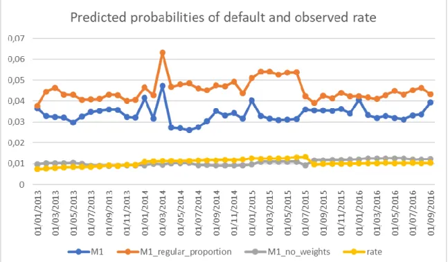
6.4 Graphical predicted default rate – JOSÉ ... 69

6.5 Predicted default rate – HENRIQUE, JOSÉ ... 72

7. Conclusion – ACHILLE, ROBERTA ... 73

8. Next Steps – HENRIQUE, JOSÉ, ROBERTA ... 73

9. Limitations - ROBERTA ... 75

Appendix ... 77

Appendix A – Structural Credit Risk Models ... 77

Appendix B –Analysis of the created variables ... 78

Appendix C – List of Variables ... 91

Appendix D – Loss Graphs ... 93

Appendix E – Variable Significance ... 94

Appendix F – Variable Impact ... 98

Appendix G – Metrics and ROC curve... 106

Appendix H – Predicted Default Rate Analysis ... 108

Appendix I – Alternative Methods... 111

Appendix J – Structured Finance Portal – ALL GROUP ... 113

1.1 - Key Differentiators Explanation ... 113

1.2 - Credit Migration Probabilities on the Tranche ... 114

1.3 - Filters on Market Performances ... 115

3 1.5 - Transition Matrix ... 117 References ... 118

4

Abstract

–

ROBERTA

As a consulting project, we were proposed to develop a neural network (NN) to

predict mortgage states in one year, based on the paper ‘Deep Learning for Mortgage

Risk’ by Justin A. Sirignano, Apaar Sadhwani, Kay Giesecke (2018). We developed a neural network model with the aim of being able to capture the relationships between the different variables, with respect to each other and to the response variable (the loan status in 12 months), better than traditional classification methods, such as logistic regressions, which constitute the benchmark set. Data was provided by Moody’s,

relating borrower, property and loan/financing characteristics for several mortgages over several periods in time (over 350 thousand mortgages). The purpose of our model is to predict the probabilities to transition to different states at a certain point in time. The best results were obtained with a 10 layer, 500 nodes per layer network. The model can identify a large portion of defaults. At the cost, however, of a general overestimation of the default rate over the years. The capability of identifying loans that will be in arrears is also acceptable, with, again, an overestimation of the verified rate. Variables relating to borrower characteristics and history as well as financing are found to be the most significant.

5

Executive Summary

–

ALL GROUP

This project investigates whether a deep learning model (a type of neural network) can be useful to predict the performance of a pool of mortgage loans. In traditional econometric models, the relationship between explanatory and dependent variables is constrained by the functional form of the model itself and by the limited data transformations that can be incorporated (squaring variables, logs, etc.). Those models may thus be insufficient to fully capture the complexity of the relationships between dependent and independent variables. In contrast, neural networks are well suited to capture complex non-linear relationships in the data.

Our work is mainly inspired by the paper “Deep Learning for Mortgage Risk”, by Justin A. Sirignano, Apaar Sadhwani, Kay Giesecke (2018). One of their main findings was precisely the existence of non-linear relationships in the data. They found that the most important component of this non-linear relationship was the interaction between the variables, meaning that the sensitiveness of the loan performance to one variable depends on other variables.

In this report, we aim at developing a non-linear deep learning model and replicate the promising results in Sirignano et al. (2018). Our dataset was provided by

Moody’s and, due to hardware constraints, a small sample of 20 000 loans (out of 350 thousand) was randomly extracted. Several other filters were applied to the sample, such us guaranteeing all loans to have 24 consecutive observations, as well as to the construction of some variables. These are detailed in section 4.

From more traditional literature (section 3.1), we found that variables are usually categorized as borrower, financing (loan) and property, with some papers also trying to

gauge how macroeconomic conditions can affect borrower’s behavior. Sirignano et al.

(2018) find evidence for strong macro effects, namely the unemployment rate, which is the most significant variable for explaining states transition.

Other papers and Moody’s recommendation, due to good performance logistic

regression, considered Loan age and Current LTV to have strong ability to differentiate the different states: default, prepayment, delinquency and performing. As well as these, we created other interaction variables we found relevant, namely Completion

6 (percentage of the contractual length of the loan already completed). The created variables are detailed in section 3.2.

The best results were obtained with 10 layer-network, trained over 800 epochs, using mini-batch stochastic gradient descent (SGD). Since there is a severe imbalance between classes in our dataset (with “performing” being the dominant class), an artificial weight (twice the inverse proportion of each class) was applied during optimization. The full model mechanics and specification are detailed in section5.

Our results reveal that borrower related risk factors, namely income related

factors, such as the proportion of delinquent balance compared to the borrower’s

income and installments as a proportion of income, as well as stability (employment status), are important at predicting the future state of the loan. Past information about the borrower, namely court related events and previous defaults, also prove to be significant (section 6.1 and 6.2 details the results, in section 6.1 we found the most significant variables – worse performance when omitted)

There is a general overestimation of the default probability by our model. Still when analyzing the receiver operating characteristics (ROC) curve (Section 6.3) we can see that a decision rule can be made to identify transitions to default and delinquency well, from originally performing loans. The overestimation can also be seen in section 6.5 where the predicted default rate is plotted against the actual one (across time).

Since our model was best at predicting defaults, analyzing the transition from performing to default state became the focus in section 6.4. Different variables were assed. Interesting patterns can be observed in the predictions. For instance, the higher estimated probability of default in situations where principal payment is delayed, indicating that agents with low home equity have higher propensity to default. The contrast between geographic regions, that is, mortgages from specific areas are more prone, to enter in default, according to our model, indicating that the property related risk factors (in this case location) can also be a differentiating factor (although not found as crucial in section 6.1 proved to have close relation with the probability of transitioning to default – section 6.2). More variables are discussed in section 6.4.

7 Given that the process to obtain an optimal network specification is an iterative one, we were constrained by the time necessary to train the model, so only a few iterations were possible. Hardware constraints also made it difficult to use a larger sample, which would likely reveal more general patterns (more in section 9).

M1 (our final model) is still a very imperfect model and further steps may be taken in order to improve on it. These relate to: the way the sample is obtained (pooled cross-section); the way the variables are encoded before being used to train the model (normalization would be preferred to the current method); the necessary iterations through possible network specifications (parameters that need to be manually chosen), with preference for larger networks (large amount of nodes and layers) which we found to work better during our testing. Research on the methodology to assess the significance of variables would also be beneficial, since it is too costly to simply retrain models without them. Finally, an ensemble model, which would combine the strengths of different networks (more details in section 8).

There are also possible alternatives to our framework, namely the use of decision trees, which allow for an easier identification of the importance of each variable, and the use of a recurrent network which would work with panel data (tracking observations belonging to the same loan) and not a pooled cross-section. Appendix I touches on these 2 methods.

8

1.

Approaches to Credit Risk Modelling

–

FILIPE

In this section, we will start by covering briefly the conceptual corporate credit risk model approaches, namely the two big classes: Structural and Reduced-Form models. Afterwards, we will discuss, with more detail, the residential mortgage risk, particularly the difficulties to model it and the conceptual loan-level models applied to measure and manage this type of loans. Finally, we will cover the new techniques, namely the machine learning models and how can they be used to evaluate residential mortgage risk.

1.1 Corporate Credit Risk – FILIPE, HENRIQUE

The concerns towards credit risk exposure are relatively recent, although the banking institutions are present in the global economy for a long time. The first class of

credit risk models was born, in the late 60s. In fact, the Altman’s Z-Score (1968) and other credit scoring models assigned a score to companies according to their bankruptcy risk, based exclusively in their financial information. The fact they were not considering market information was the biggest flaw of this type of models, moreover they did not

estimated the probabilities of default: “it may indicate that the mortgage is likely to

default, but it does not tell how likely it is to default (i.e., whether there is a 90 per cent

or 60 per cent probability of default)” (Li, M.; 2014).

The importance of the market information started to be noticed, and the first generation of structural market-based credit risk models appeared in the seventies, especially after 1974, when it was founded the BCBS, the Basel Committee on Banking Supervision. These models are known as Structural models since they relate the credit risk management to fundamental variables, such as the firm assets’ value: if the assets

become lower than the liabilities, the firm will default. They attempt to price the credit risk, i.e., the price of the exposure and they are based in the option pricing models: Black

Scholes’s and Merton’s models. Although they give some good insights to compute

probability of default, their assumptions are too strictly and hardly hold in the real world, considering, for instance, non-stochastic interest rates; too simple capital structures; and default occurring only at maturity.

9

The second generation of structural models was born from changes to Merton’s

model to accommodate less strict assumptions, for example, they started allowing for default before maturity and using stochastic processes to define interest rates. However, these models, have a low number of inputs failing to capture some information and generating poor performances, in certain scenarios. Despite the limitations, structural models are broadly used in the corporate credit risk industry, such

as Moody’s-KMV Portfolio Manager, Credit Metrics, or Credit Portfolio View. (a brief information regarding these models can be seen in Appendix A.

Their application in mortgage risk estimation is not so frequent, even though, Cunningham & Hendershott (1986) applied “the Black and Scholes (1973) option pricing

model as modified by Brennan and Schwartz (1977)” in order to analyze the default risk

of different types of mortgages and loan programs and, in the last instance, to compute the optimal default premia Federal Housing Administration (FHA) should charge to different borrowers.

The other class of credit risk models is the Reduced-form, which contrasts deeply with the structural approach. Instead of having the probabilities of default derived from

the assets’ value, the default event is considered exogenous, this way the probability is derived from a random variable that follows a Poison distribution. The default will

happen if this “exogenous random variable jumps instantaneously from one to another at random times”, (Zhang, X.; 2017). In fact, nowadays, we are able to use reduced-form models that make predictions over several periods, that focus on time-varying covariates, instead of static covariates. This type of models uses this statistic based stochastic process, instead of a typical theoretical model, being, then, less dependent on assumpions. One example of a reduced-form model is the CreditRisk+, used by Credit Suisse. This model is pretty easy to implement but has the disadvantage of only consider default state besides performing; then it only computes the default probability, ignoring all the other rating levels.

10 As we have discussed, the focus of our project is mainly related to private mortgage loans, this is, loans borrowed by householders to finance real state acquisition. Residential loans’ risk is not so easy to measure as corporate loans’ risk, since individuals’ information is not accessible in the market. This information unavailability

is a big constraint when building a residential mortgage risk model, however there are other characteristics that make quite hard to analyze, measure and manage residential

mortgages lenders’ exposure.

Firstly, it is necessary a lot of scenarios to capture all the possible borrower behaviors (loan status) in different economies. The loan-level behaviors are not homogeneous, in other words, in different economies, there are strong evidence of different performances and correlations, for the same loan. The mortgages loans performance is much more dependent on the economic state than commercial loans and the volatility is relatively higher as well. Summarizing: one loan can have different behaviors according to the economic scenario and different loans, in the same scenario, can present very different performances.

Secondly, and like most of the loans, the mortgages are path dependent instruments. This means that loan history (historical information and performance) is relevant in future performance, and the past and current behavior will have a tremendous impact in future behavior. Thus, mortgages analysis requires a multi-period model.

Lastly, mortgages may have also call and put options: option to prepay and option to run away, respectively.

Nevertheless, there are some models broadly used to study mortgage risk, they are divided in Loan-level models and portfolio level models, according to the scope of the analysis, the implementation, and the data used.

A Loan-level model, as the name indicates, would be suitable to study the performance of individual loans. The input, usually, relies on borrower and mortgage individual information (instead of macroeconomic data) and the output is the loan’s

default probability, that eventually could be aggregated in order to estimate the loss of a given portfolio.

11 On the other hand, a portfolio-level model is applied when we want to study the default rate of a mortgage loans portfolio, as a whole. The interaction between the loans (i.e. correlation) is quite significant, this way, the data is mainly composed by macroeconomic explanatory variables, and less by borrower or mortgage individual information. In general, the inputs of the portfolio models are aggregated, this is, each input of the portfolio model is the weighted average of the inputs of each individual loan that composed the portfolio. For instance, the LTV ratio of the portfolio model will be

the weighted average of the individual loans’ LTV ratios. A similar situation occurs with the output: it is obtained the portfolio’s probability of default, instead of the loan by

loan probabilities.

Bottom line, we can infer that portfolio models are more restrictive than loan-level models: the losses predicted by a loan-loan-level model can be aggregated in order to obtain portfolio loss, whereas the portfolio output cannot be insulated.

Thus, in these sub-sections, we will focus on explaining and analyzing the advantages and disadvantages of four widely used loan-level mortgage risk models:

1.2.1 Linear Regression

The first model developed to study mortgage risk was a basic linear regression, in which the default risk of certain loan, known as Loan Status, - the dependent variable that takes the value of 0, if it defaults, or 1, if not - is determined by k independent variables. The model follows the regression:

𝐷𝑒𝑓𝑎𝑢𝑙𝑡 𝑟𝑖𝑠𝑘 =∝ +𝛽1𝑥1+ 𝛽2𝑥2+ ⋯ + 𝛽𝑘𝑥𝑘+ 𝜀

Where ∝ is the constant, 𝑥𝑖 are the variables that try to explain the default risk, 𝛽𝑖 the linear coefficients, that measure the sensitivity of default risk to a change of certain magnitude in the 𝑖𝑡ℎ _{explanatory variable, and 𝜀 the error, this is, what is not} explained by the model.

This model is quite simple and easy to implement: from a sample analysis, it estimates the value of the coefficients that, posteriorly, are used to predict the default risk of a specific loan. Moreover, both panel and cross-sectional data can be used, and

12 the coefficients and output are interpreted in a straightforward way. For instance, the significance tests are pretty much easy to perform.

Still, the main problem of this model is the linearity assumption; according to it, even if the default determinants are transformed before joining the regression (for instance, through a log transformation), the relationship between the dependent and the explanatory variables is assumed to be linear. However, there are evidences of non-linear relationships between borrower behavior and the variables, which this non-linear model fails to capture, as it will be proved in section 3.2. The main reason we are building our machine learning model is to overcome this problem.

Other issue is related to the dependent variable, the default risk. This is not the default probability but a proxy, that can be seen as the predicted Loan Status. Instead of giving us a number between zero and one, the model outputs the 0, if it predicts default, or 1, otherwise. Thus, the model assumes only two scenarios: Default or No default, ignoring, in a certain way, how much close (or far) the mortgage seems to be from defaulting.

1.2.2 Logistic Model

The logistic model is an improvement to the linear regression, solving some of its problems. The logit model, as it is broadly known, applies a positive monotonic transformation to the linear regression, through the following logit formula, transforming its output in a default probability.

𝑃𝑟𝑜𝑏𝑎𝑏𝑖𝑙𝑖𝑡𝑦 (𝐿𝑜𝑎𝑛 𝑆𝑡𝑎𝑡𝑢𝑠 = 1) = 1

1 + 𝑒−(∝+𝛽₁𝑥₁+𝛽₂𝑥₂+⋯𝛽_𝑘𝑥_𝑘)

Where the dependent variable is the probability of default (status equal to 1). This formula is applied when we have got a binary dependent variable. For instance, we were considering only two loan status, the mortgage could default (loan status=1) or do not default (loan status=0).

However, in real world, when accessing the credit risk, a mortgage may assume different categories within the non-default class: performing, delinquent and prepaid. Thus, the dependent variable is not binary anymore, and to incorporate more than two

13 states we can use a multinomial logistic regression, which will not be developed in this paper, once it is a complex procedure and not common to implement. So, logit model does not necessarily limit us to a simple binary framework.

𝑃𝑟𝑜𝑏𝑎𝑏𝑖𝑙𝑖𝑡𝑦 (𝐿𝑜𝑎𝑛 𝑆𝑡𝑎𝑡𝑢 = 𝑗) = 𝑒

(∝+𝛽₁𝑥₁+𝛽₂𝑥₂+⋯𝛽_𝑘𝑥_𝑘) 1 + 𝑒(∝+𝛽1𝑥1+𝛽2𝑥2+⋯𝛽𝑘𝑥𝑘)

Campbell & Dietrich (1983) applied a multinomial logit regression to access residential mortgage risk.

Most of the mortgage papers applies logistic regressions. As discussed above, logit model overcomes some challenges of the linear regression, not only in extending the status the mortgage can be considered in, but also regarding the outcome, in the sense that this model, contrary to the linear regression, give us the prediction of how close a loan is from default, measured by the probability of default. In testing the significance of the explanatory variables, both models give similar outcomes.

Nevertheless, the positive monotonic transformation of the linear regression does not relax the linearity assumption. This way the flaw persists: under the logistic model, the logarithmic function of the odds is a linear function of the explanatory variables. This may have implications in fitting specific datasets, for example, an explanatory variable, having a significant non-linear relationship with default probability may be wrongly excluded from the model, due to lack of significance.

Failing to capture the non-linearity relationship sometimes can be mitigated by including in the regression the squared-term of the variable and cross-terms with other explanatory variable, or even by using categorical and dummy variables; however, these are not fool proof methods, and do not guarantee the overall non-linearity effect capture.

1.2.3 Survival Analysis

Survival analysis is an alternative method for the previous models. This analysis gives a special emphasis to the life course of the mortgage.

As we discussed before, a mortgage can be marked as performing, delayed, prepaid or default. These loan statuses are mutually exclusive, meaning that, at each

14 point of time, the mortgage loan status can be one and only one of these states. However, over, the time, the status can change across categories, in accordance with the borrower behaviour. It is frequent a loan, that starts by being performing, enters in delinquency, in default or gets prepaid.

Survival analysis in precisely studying this relationship between loan status and time passage, more specifically, how long a mortgage survives, i.e., the time it takes to migrate from performing to default or delinquent. Note that delinquency risk is not considered under the assumptions of this model and default and prepaid are assumed absorbing states, after reaching one of these states the mortgage will remain with that state, thenceforth.

The conditional probability of survival until t, also known as hazard rate, is defined by the following expression:

ℎ(𝑡) = ℎ0(𝑡)𝑒(𝛽1𝑥1+𝛽2𝑥2+⋯𝛽𝑘𝑥𝑘)

where, 𝑡 is the loan age, ℎ0 is the empirical baseline hazard, which captures the shape of the hazard function, according to 𝑡. Like the previous models, 𝑥𝑖 are the explanatory variables and 𝛽𝑖 the coefficients, that studies the impact of each variable in the conditional probability of survival. This formulation assumes a discrete approach to time, the continuous would have ℎ(𝑡)∆𝑡, as dependent variable.

Green & Shoven (1986), for instance, looked over mortgage and borrower variables and try to predict which of them may contribute to a default, in a defined time period.

Elul et al (2010) estimated a dynamic logit model (explained in the last section), using a hazard function varying nonparametrically, applied typically in these survival

models. In fact, “survival analysis models (namely the Cox regression) and logistic regression models sometimes include quadratic or other nonlinear transformations of

certain variables” (Sirignano et al.; 2018). The Cox proportional hazards model, referred

before, is one category of survival analysis that “allows to analyze the effect of several

risk factors on survival”, and may include a nonparametric baseline hazard function in

15 One advantage of the survival analysis is the fact that it can be structured to capture each one of two types of mortgage risk: default risk and/or prepayment risk. As it will be explained further in section 2, both termination risks, even being mutually exclusive, should be considered by the lender, since a default or prepayment event will impact his cashflows.

Deng et al. (2000) included alongside both termination options estimations: for prepayment and for default and estimated the unobserved heterogeneity (“risk preferences and other idiosyncratic differences across borrowers”) of the borrowers,

that seems to be meaningful.

This matching between the loan age and the termination event is quite important and extends the typical frameworks, since it is not only being studied the impact of the conceptual determinants in the probability of the event of interest, but also the impact of the life course of the mortgage, i.e., the model is formulated to generate the probabilities as a function of loan age and the other explanatory factors (also assumed by logistic and linear regressions). The time horizon, trough survival is flexible from loan to loan, contrary to the logistic regression, in which each estimation process generates the default probability for a specific (fixed) time period.

Other advantage of the survival analysis is the incorporation and adjustment of

‘censored data’ in the estimation procedure, while the logistic model would abandon

the observations for unavailable information. The assumptions of survival model are also quite flexible, when estimating semi-parameters such as the hazard baseline.

The main problem of this analysis in related to the data handling: firstly, the data be difficult to treat, secondly, the output analysis could require some developed programming techniques. These are the main reasons this model is not broadly used, in practice, although the good predictions it generates.

1.2.4 Optimization model

The previous three models are statistical models, the estimation procedures applied are related to the fundamentals of statistics, such as linear regressions and logit transformations. The following model is an economic model, in the sense that it is structured to capture the economic decision behind the termination event. Even though

16 this is not statistically related, we are going to study this model, once it can help us to understand the economic reasoning of certain determinants that may impact the borrower behaviour, and even which explanatory variables we should incorporate in the machine learning model.

The optimization model assumes that a borrower takes default or prepayment decisions in a way to maximize his wellbeing, measured by his wealth and utility functions, what is equivalent to say that the borrower minimizes the costs related to the house. The borrower, in each period, will choose one of three alternatives, according to lower cost. The alternatives are: to pay the instalment, to prepay the mortgage (refinance) or to default the current mortgage. Basically, he will choose the option that generates a larger benefit to himself, i.e., that optimizes his wellbeing, minimizing the cost function.

There are several different functions to define the borrower’s choice, we opted

for the following one, according to Capozza, Kazarian, and Thomson (1996), which is the most consensual:

𝑃_𝑡(𝐻_𝑡, 𝑟_𝑡) = min [𝑃_𝑡𝑑(𝐻_𝑡, 𝑟_𝑡), 𝑃_𝑡𝑝(𝐻_𝑡, 𝑟_𝑡), 𝑃_𝑡𝑐(𝐻_𝑡, 𝑟_𝑡)]

We will not do an exhaustive analysis to this function, but rather understand the importance and the limitations of this type of models. Summarizing the function, the cost of the house for the borrower, in each month, given by 𝑃_𝑡(𝐻𝑡, 𝑟𝑡), will be the lowest cost among the previous three alternatives: defaulting, 𝑃𝑑, prepaying the current mortgage and refinancing, 𝑃𝑝, or performing the current mortgage, 𝑃𝑐.

The cost, in each alternative, depends on the current house value and on the interest rate payed, in each month, defined by 𝐻_𝑡 and 𝑟_𝑡, respectively. These explanatory factors are estimated, in each month, 𝑡, in several scenarios, through stochastic processes, that, afterwards generate the decisions distribution, from where is computed the probability of each state.

The model follows a simple framework that can eventually include other determinants of default, for example, the monthly income or the loan age. There are

17 unemployment. However, these variables selection process needs to be done carefully since the estimations are quite sensitive to inputs, then, bad assumptions may distort the outcomes of the model.

Optimization models link the borrower behaviour to economic forces, depending less on loan historical data, what can be positive, if we have poor information on loan.

On the other hand, since they are not statistically-heavy, economic models require developed programming to make predictions, and this is what makes the implementation harder when compared to statistical models. Not considering the delinquency scenario, in the decision process, can be seen as a caveat; moreover, the assumptions made in order to compute the cost under each decision, 𝑃𝑖, is relatively subjective.

We feel important to reinforce that the model (i.e. equation) studied is one of the several optimization models developed. There is literature that uses the utility maximization approach, instead of cost minimization, in which they “define household

utility as a function of non-durable consumptions over time, housing consumptions over

time and/or terminal wealth (financial wealth and housing wealth)”, Li, M. (2014).

1.3 Deep Learning Models and credit and liquidity risk - ACHILLE

Due to the nature of their business, banks have plenty of data on their customers. However, many of them struggle with the stochastic behavior of their customers and misevaluate their credit risk, which can lead to inaccurate estimations of their liquidity

buffer’s need. Yet a correct management of liquidity risk is key since banks are required

to maintain a healthy balance between investing to maximize their shareholders’ profit

and maintain high liquidity levels to respect their obligations to depositors (Tavana, et al., 2018). Moreover, as seen in previous examples, mismanaging liquidity and

misevaluating credit risk can lead to the bank’s failure. Too little liquidity and you risk insolvency, too much and you risk inefficiency (Matz, 2007).

The models from last section fail to capture the non-linear relationships between

the borrowers’ behaviour and the explanatory variables. Moreover, the correlation between variables can be harmful to prediction, resulting on bad performances and

18 misevaluation of credit risk. A machine learning model would overcome this conceptual

models’ limitations. In fact, artificial intelligence (AI) and machine learning models are being developed to model credit risk, not only for corporation loans but also for residential mortgages.

The subject of Deep Learning’s use for credit risk assessment and management

has been widely studied in the academic literature (Barboza, Kimura, Altman; 2017) (Huang, Liu, Ren; 2018) (Angelini, Tollo, Roli; 2008). Tavana, Abtahi, Di Caprio and

Poortarigh have researched the potential positive impact deep learning’s techniques

could have on banks’ liquidity risk measurement and management (2018).

Tavana, Abtahi, Di Caprio and Poortarigh found that neural network’s technology can detect better liquidity risks’ occurrences using data available in any banks’ balance

sheet. In addition, as neural network can deal with very noisy data and missing values (Angelini, Tollo, Roli; 2008), their use does not require extensive preprocessing of the

data, facilitating the job of banks’ managers (Tavana, Abtahi, Di Caprio, Poortarigh;

2018).

1.3.1 Corporate credit risk evaluation

There is also an extensive literature on how deep learning models can improve

corporate credit risk’s evaluation (Zhao, Xu, Kang, Kabir, Liu; 2015) (Khashman; 2010). Among the most praised assets of deep learning models are their ability to predict credit

events with high accuracy, despite restrictive conditions, such as variables’ endogeneity,

an important number of outliers and missing values. The results found in the literature continuously showed these models achieved better results than traditional ones such as (Tavana, et al., 2018) logistic regressions (Angelini, Tollo, Roli; 2008)), and have also proven successful in credit scoring using only CDS data (Luo, Wu, Wu; 2016).

Furthermore, SMEs are more likely to fail due to short-term difficulties rather than long-term characteristics (Carton & Hoffer; 2006). In the context of their credit assessment, considering the constantly changing nature of many explanatory variables is therefore key, and deep learning models have proven successful in incorporating information on short-term evolutions of variables (Barboza, Kimura, Altman; 2017). The suggested improvement in credit assessment’s accuracy despite restrictive conditions

19 improvements in predictions accuracy can largely improve their profitability while

reducing their balance sheet’s portion of Non-Performing Loans. As for SMEs facing financing problems due to their complexity or lack of data to hand-in, deep learning models could facilitate their credit profile evaluation, which would in turn give them access to funding (Huang, Liu, Ren; 2018).

1.3.2 Private Loans credit risk evaluation

Sirignano et al. (2018) have expressed the need to use this technology to evaluate mortgage loans by showing the highly non-linear relationships existing

between borrowers’ behaviors and risk factors, and proving the interactions existing

between the explanatory variables. They found that prepayment events in particular, are significantly affected, looking at their relationship with the difference between initial mortgage rate and market rate. As for the interaction between explanatory variables, they illustrated this phenomenon with the impact of a borrower’s FICO score 1 _{on the}

explanatory power of unemployment rate. Following these results, they questioned the use of more traditional models based on linear interpretations and suggested the use of deep learning techniques to predict mortgage loans’ behavior. The neural network they

developed on a very large US data base have proven very successful.

Additional research on private loan credit risk

Training a neural network on consumers’ credit card data have also proven to give excellent credit risk predictions. Focusing on these transactions and excluding other data usually considered in credit scoring (i.e. socioeconomic data, loan balance and payment history, or credit bureau data), Kvamme, Sellereite, Aas and Sjursen managed to build a neural network predicting accurately mortgage defaults in Norway (2018). Eventually, to counter the problem of delicate and rare situations in credit scoring, normally assessed by human experts, an emotional neural network has been developed and once

again has proven successful. Its two “emotional” responses, anxiety and confidence,

change during the learning phase. As the loss function decreases meaningfully, anxiety decreases, and confidence increases (Khashman; 2011). This aspect of emotional neural networks allows for interpretation of data inputs with a degree of confidence. All the

1 _{Fair, Isaac and Company. A data analytics company focused on credit scoring founded in 1956 and} based in San Jose, California: https://www.fico.com/en/about-us (Last assessed in December 2018).

20 results justify the need to investigate further the use of deep learning technology to improve credit and liquidity risk evaluation and management.

21

2.

Transition states

–

FILIPE, JOSÉ, ROBERTA

There are four possible states a mortgage can be in:

• Performing: all payments occur as predicted by the contract.

• Prepayment: A mortgage is considered prepaid when the borrower decides to partly or entirely (the one we will focus on the paper) pay in advance the principal of the loan.

• Delinquent: A loan is considered delinquent (or in arrears) whenever the payment is not made within one month from when the instalment was due.

• Default: A mortgage is considered in default when the cumulative amount in arrears is higher than three monthly installments (i.e. +90 days cumulative delay).

Section 4.1 will further explain how we applied this to our data. This is, how these classes were built and how observations were classified.

2.1 Default and Prepayment risk

An important role is given to the default and prepayment classes. These two statuses are extremely relevant to the lender. Whenever the mortgage is behind payment or is prepaid the lender experiences a disruption in cashflows from the missed payments.

Default occurs when the counterparty fails to meet its contractual obligations. The likelihood of this happening is called rate of default and it is one of the most important parameters to define the credit exposure of the lender. In this paper, the rate of default is calculated monthly, over twelve-month horizon (Sections 4.1.5 and 4.1.6). Thus, the monthly rate of default describes the likelihood of a mortgage to default within the following twelve months. The time horizon was set to twelve months as nowadays it is widely used in the financial industry for the calculation of credit risk and related

22 capital requirements. Moreover, the IFRS 9 requires impairment of financial assets to be measured as the expected credit losses over a twelve-month horizon2_.

Therefore, during the process to calculate the monthly rate of default, a new column with the twelve-month lagged mortgage status was added in order to have for each month the number of loans that defaulted within the next twelve months.

By the same token, whenever a mortgage is prepaid, the lender would lose either partly or entirely his future interest cashflows. With a decrease in current rates in the market, mortgages loans are paid off earlier in order to incur in lower interest rates by refinancing the loan, and the lender would have to deal with reinvestment risk. Prepayment is perceived as a financial risk as the investor would not be able to reinvest the cashflow at the same rate of return as the one locked in the mortgage and would have to use the current market interest rate. The mortgage can be partially prepaid in case the borrower wants to pay less in interest rates and prefer to pre-pay part of the principal amount.

A mortgage consists of a straight bond and an option that gives the borrower the right to prepay and refinance the loan at any time. The decision of prepay can be considered as a call option exercisable on the mortgage by the counterparty, giving the right to the borrow to redeem the mortgage before the maturity date3_{. The call option}

would be exercised whenever the value of the future instalments exceeds the value of the balance and the cost of refinancing the loan, both explicit costs, such as fees, and implicit costs, such as costs incurred when asking for another mortgage. However, as already seen in other studies conducted on prepayment risk, the behavior is unpredictable since it can be caused by other factors linked to the single borrower.

Understanding the behavior of prepayment would be profitable to the mortgagee, to decrease his exposure to prepayment, reinvestment4 _{and liquidity risks.}

Liquidity risk is especially important for banks, which have to correctly estimate their

2 _{“The rate of default under IFRS 9: multi-period estimation and macroeconomic forecast”, Tomáš} Vaněk, David Hampel, 2017

3 _{“Modelling Prepayment Risk”, J.P.A.M. Jacobs, R.H. Koning, E. Sterken, 2005} 4 _{“Modelling Prepayment Risk”, J.P.A.M. Jacobs, R.H. Koning, E. Sterken, 2005}

23 liquidity profile, strongly influenced by the maturity of their assets and liabilities5_,

consult section 1.3 for more information on this subject.

24

3.

Literature and new Variables

3.1 Overall analysis – FILIPE, JOSÉ

Our dataset comprises 56 different Variables, some with dynamic and other with static features. Some of these variables are extensively discussed and studied, in the mortgage risk related literature, due to their explanatory power regarding the borrower behavior.

In addition to the provided variables, Moody’s recommended the creation of

new interaction variables, namely Loan Age and Current LTV that were proven to have high explanatory power in the logistic regression estimation, tackling the same issue.

The variables try to capture the different types of risk a lender may be exposed to. Von Furstenberg (1969) and Gau (1978), group the risk factors in three areas: borrower and property developed by, who considered three major determiants: loan financing, borrower, and property. Financing risk factors try to gauge potential disruption to payments originating from the loan contract, such as the loan amount, balances, term, loan-to-value (included in our modeL: CurrentLTV, PaymentFrequency, Completion, LoanTermInMonths among others – see appendix C for full list of variables)

Borrower risk variables try to capture the risk related to borrower’s information,

such as his age, the occupation or the income. In fact, income is established as an important influence factor, translating the level of wealth, one of the most important characteristics when assessing borrower risk (ability of the borrower to meet the commitments agreed) (Gau, 1978).

Finally, property risk variables try to capture the influence that the underlying property can have on the performance of the mortgage, for instance, how the borrower behaves as his house gets more deteriorated. Property type or Valuation Volatility are examples of variables linked to property risk we are using in our model.

Vandell, K. (1978) and Webb, Bruce G. (1982) extend on the variables used, giving also importance to the relationship between instalments and income (included in our model as well – Installpropincome) income sources as risk of delinquency.

25 The project was mainly based on Sirignano et al (2018). On it, data related to borrower, property and loan financing characteristics is used as well as local and national economic variables such as unemployment and lagged default rate. Some of these variables change during the life of the loan, others remain constant. Our dataset also covers borrower, property and loan financing characteristics with variables such as

AgeOfBorrower, PropertyType and CurrentInterestRate for each category respectively. As in Sirignano et al. (2018), some refer to the origination of the loan and remain constant through the life of the loan others are updated with every observation. Economic variables such as unemployment are not included, with the date (as distance form year 0) being the only proxy to mirror the economic reality of the particular year and month of an observation. It is unclear if the inclusion would be of much value. One of the contributing factors for these macroeconomic variables to be so significant in Sirignano et al. (2018) is tied to the large time period the observation range in and the sample, on which we worked on, ended up ranging only from 2013 to 2017.

Like Sirignano et al. (2018), we also have a data’s static-dynamic division,

following what was done in Moody’s dataset. We have some variables that were evaluated at mortgage’s orgination and others that are change on a monthly basis. For instance, Interest rate type or Geographic region (of the property) are considered static variables while Current LTV or Distance to Maturity.In fact, we also transformed the static variables in dynamic by interacting different types of variables.

However, contrary to Sirignano, we do not study the macroeconomic factors, in our analysis. As referred before, the only economic factors that may have implications in our neural network are: the YrM, the observation month, that may be influecned by macro factors, and the United Kingdom House Price Index, used to build the Current LTV. (section 3.2.1 – Current LTV).

In fact, as explained in section 1.2, a loan-level model relies more in borrower-level variables than in macroeconeomic determinants of default. Although, the inclusion of macroeconomic explanatory variables in the model increases the model’s overall

fitness and performance. Moroever, there are evidences of some macroeconomic variables having the highest explanatory power in borrowers behaviour, like the state

26

unemployment rate, or the interest rate margin, the difference between borrower’s and market’s interest rates. (Sirignano et al.; 2018)

3.2 Created variables

3.2.1 Ability to cover the loan with the property value – ACHILLE E FILIPE

The group wanted to capture the impact of the value of the house on the loan

states’ probabilities. We believed considering this amount in proportion to the

remaining loan value to be paid – ending pool balance – should allow the capture of how much a borrower is covered by the value of her house. As a result, we analyzed the current Loan-To-Value as well as a similar variable considering the last official valuation. We thought of creating these variable after having found in the literature that, as the value of the house increases, the rate of being performing should increase (Bian, Lin, Liu; 2018). In addition, high changes in the property value largely affect the default probability (Kelly, McCarthy, McQuinn; 2014).

Current Loan-to-Value Ratio

Original LTV, defined by the loan value divided by the house price, both at origination, was one of the static variables initially considered. However, this ratio is not considering the macroeconomic factors over time, which have an implication in the house price, neither the fact that loan value is changing over time, according to what has been repaid. In several papers, it has been emphasized the impact of house prices and home equity accumulation in the default event.

For these reasons we created the Current Loan to Value (Current LTV), which transforms original LTV in a dynamic variable, capturing the loan value and the house price, in each month.

𝐶𝑢𝑟𝑟𝑒𝑛𝑡 𝐿𝑇𝑉𝑡 =

𝐸𝑛𝑑𝑖𝑛𝑔 𝑃𝑜𝑜𝑙 𝐵𝑎𝑙𝑎𝑛𝑐𝑒_𝑡 𝐶𝑢𝑟𝑟𝑒𝑛𝑡 𝑉𝑎𝑙𝑢𝑎𝑡𝑖𝑜𝑛𝑡

27 The Current LTV, in each month, takes the current loan valuation, defined by the

loan’s ending pool balance and divides it by the Current House Valuation, which was

computed considering the UK Government House Pricing Index (HPI), considering the following formula:

𝐶𝑢𝑟𝑟𝑒𝑛𝑡 𝑉𝑎𝑙𝑢𝑎𝑡𝑖𝑜𝑛_𝑡= 𝑉𝑎𝑙𝑢𝑎𝑡𝑖𝑜𝑛_𝑡−𝑛∗𝐻𝑃𝐼𝑡−𝑛 𝐻𝑃𝐼_𝑡

We feel important to refer that it was considered the overall UK HPI, regardless

houses’ specific locations.

The Current LTV, according to several studies, is one of the most important factors in explaining the borrower behavior. This variable tries to capture the effect of the house finance strategy, in each month - the percentages of debt and equity financing the house - in the loan states’ probabilities. The LTV has a positive impact in probability of default and a negative impact in prepayment probability. (Campbell, Tim S., and J. Kimball Dietrich; 1983)

In Von Furstenberg, George M. (1969), although not developed, it is suggested to include a cross-term variable relating the income level and the LTV ratio, being expected a higher probability of default for borrowers with low income values and higher LTV ratios. This would be interesting to do.

However, the Original LTV also has been considered as a significant variable to explain borrower behavior, in particular default. Recently, Campbell, John Y., and Joao

F. Cocco (2014), incorporated this original ratio in their household’s utility-maximization

model, which tries to predict the default decision. According to them, “a higher (initial)

LTV ratio increases the probability of negative home equity and mortgage default”.

Theoretically, the Loan to Value ratio compares the mortgage amount with the appraised value of the respective property. A higher mortgage relatively to the house price will make the borrower more dependent on debt to finance his house, and consequently more susceptible to do not comply with his obligations. Therefore, following the related literature, the lenders usually consider loan with higher Loan to Value ratio riskier than loans with lower LTV and, in order to protect themselves against

28 the exposure, they will increase the borrowing cost, meaning they will set higher interest rates on mortgages with high LTV ratios.

Considering a small sample of loans, we computed the median of Current LTV, given us approximately 0.46, meaning that, on average, within this sample, each

mortgage, on each month, supports around 46% of the house’s value. We chose to use

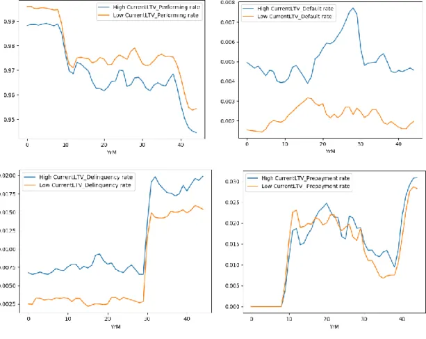
the median instead of the average because it is better excluding outliers. Then, we divided the observations in two sets: High LTV and Low LTV, considering if they have a Current LTV above or under the median, respectively, and we computed the observable rate of each state, for both LTV levels, in each month.

On the one hand, we can observe that Current LTV seems to follow a pattern for borrower behavior, namely for performing and defaulting.

Mortgages with a lower loan to value ratio had, on average, higher performing rate, i.e. keep paying on time, and lower default rates, compared to higher LTV ratios mortgages, as it can be seen:

Figure 1

This was theoretically expected: a borrower less dependent on debt to finance his house will have a higher probability of complying with the payments, and lower probability of default the loan.

In fact, for default the aforementioned difference looks more prominent, in other words, the gap between high LTV and low LTV functions is broader than for any other state, which emphasizes the explanatory power of default probability by Current LTV, i.e., Default levels are more sensitive to changes in LTV (Von Furstenberg, George M.,

29 1969). Important to refer that a higher LTV does not mean that the borrower is more indebted, in absolute terms, instead he is more dependent of debt to pay his house.

On the other hand, for prepayment and delinquency rates the distinction between LTV levels does not look so clear. Nevertheless, when looking to the scatter plot, which plots the Current LTV against the prepayment rate, we can observe a downward trend: borrowers with low values of Loan to Value ratio paid their commitments sooner than expected, in other words, loans with low LTV ratios were prepaid more frequently than loans with high values of LTV ratio. From delinquency scatter plot we cannot make a big inference, maybe a slightly upward trend for LTV ratios lower than 1, pointing a more frequent delaying in payments, for higher LTV values.

Figure 2

30 A studied conducted by PI Analytics, on a 50 thousand loans sample originated during 1999-2013 from Freddie Mac Loan Level Dataset, related the mark-to-market LTV (our Current LTV) with the default and prepayment probabilities. For LTVs under 1 the prepayment rate is flat near 70%. As the LTV increases, the prepayment rate starts to decrease. For LTVs above 2.25, the prepayment rate is virtually 0%. The default rate has an analogous behavior: for LTV ratios under the 1 threshold, default rate exhibits a constant flat behavior, near 0%. For LTV above 1 the default event starts to be more

frequent, “as the amount of loan increases relative to the value of the house, the

willingness of the homeowners to default on their mortgages increases”, reaching a

100% default rate, for rates above 2.25.

Besides this research, there are other papers that empathize the fact that LTV

effect on states’ probabilities kicks in after a certain LTV threshold (Li, M. 2014).

Testing Current LTV Sample 2 we can observe the same patterns found in-sample analysis, supporting the literature, especially for default and performing scenarios. The graphs can be seen in Appendix B – Figure 21.

The Current LTV is one of the main determinants of loan states’ probabilies,

therefore it will be considered in our machine learning model

Ability to cover the loan with property value – LTV with last official valuation

This variable differs from current LTV as the value of the property taken for current LTV takes the original valuation of the house and changes it according to the house price index, whereas here we take into consideration the last official valuation amount of the house:

𝐴𝑏𝑖𝑙𝑖𝑡𝑦 𝑡𝑜 𝑝𝑎𝑦 𝑡ℎ𝑒 𝑙𝑜𝑎𝑛 𝑏𝑎𝑐𝑘 𝑤𝑖𝑡ℎ 𝑡ℎ𝑒 𝑝𝑟𝑜𝑝𝑒𝑟𝑡𝑦 = 𝐸𝑛𝑑𝑖𝑛𝑔 𝑝𝑜𝑜𝑙 𝑏𝑎𝑙𝑎𝑛𝑐𝑒 𝐶𝑢𝑟𝑟𝑒𝑛𝑡 𝑝𝑟𝑜𝑝𝑒𝑟𝑡𝑦 𝑣𝑎𝑙𝑢𝑎𝑡𝑖𝑜𝑛

▪ called IncentiveToSell on the python notebook.

▪ A high ratio = a low ability, a low ratio = a high ability.

We called it ability to sell the property, from the fact that lower ending pool balance to house value would make the borrower able to sell the property to pay the loan back.

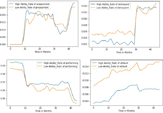
31 We divided the data into two groups to assess this relationship: the ones with higher ability to sell their house, and the ones with lower ability. The threshold used to divide

them was the ratio’s median value.

Overall, this variable analysis gave us expected results for the performing state and default state: a much higher default rate in the low ability category and a strong positive correlation between the two categories in the performing state. The high ability category outperforming the low ones. The graph below illustrates this.

Figure 4

These relationships justify the need to consider the examined variable in our neural network for its explanatory power. These observations have been confirmed when tested In Sample 2 (Appendix B – Figure 23). However, we noticed a surprising

effect of this variable’s categories on the delinquency rate. As for its relationship with prepayment, the overlapping of both categories weakens the explanatory power observed before.

Figure 5

Looking at the relationship with delinquency in particular, one can see an expected effect for the first two thirds of the time. Yet, reaching the 30th _{month, when an}

32 households savings (OECD; 2018)(BBC; 2017), the high ability category’s delinquency rate gets higher than the low one. As a result, this variable’s ability to explain

delinquency is relatively strong, but is very sensitive to chocs. As for prepayment, the graph above suggests a weak ability to explain this state. Nevertheless, despite these weaknesses, this variable use in our neural network is justified by its explanatory power for the performing and default rates.

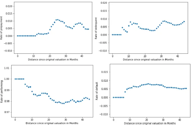
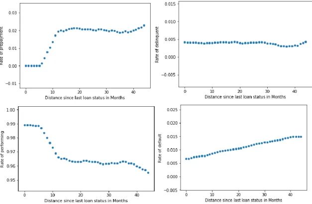
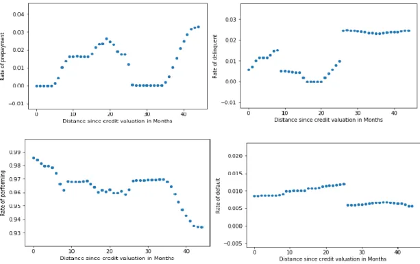
3.2.2 Time elapsed since evaluation – ACHILLE E FILIPE

Additionally, the group decided the effect of time should be considered further. Indeed, most of mortgage and other personal credit score providers insist on the

necessity to continuously update credit holders’ score (Equifax, 2018), (Experian, 2018), (TransUnion, 2018). As lenders usually report monthly data on their borrowers, the

borrowers’ credit score is therefore adjusted, and important fluctuations can happen

(NerdWallet, 2018). Having in our data inputs many dates regarding both the borrower

and the property’s valuation, we decided to create “distance” variables capturing the effect of time that passed from a certain valuation event until today. We considered the following variables:

Time elapsed since last property valuation

= Today′s date − last property valuation

▪ called DistanceFromValuation in the python notebook

Distance since original property valuation

= Today′_{s date − Original vlaluation date}

▪ called DistanceFromOriginalValuation in the python notebook

Distance since credit evaluation = Today′s date − Bureau score year

▪ called DistanceFromEvaluation in the python notebook

Distance since last loan status = Today′_{s date − Loan status′ date}

33

Looking at these variables’ relationships with the different mortgage loan’s states

(Appendix B ), together with the sole effect of time, we noticed recurring trends that we

expected, such as declines in performing loans’ rates and (in most cases) increases in

the default rates. However, what is more important in the context of our analysis with a multilayer perceptron is that the effects of the variables’ as well as the time effect are

not perfectly correlated with each other and have very distinct intensity and volatility, with relationships sometimes linear or non-linear (Appendix B). Therefore, each event’s time interval’s effect having their own specificities, their consideration represents

relevant inputs for our multilayer perceptron. The next paragraphs explain the variables’

specific effects noticed.

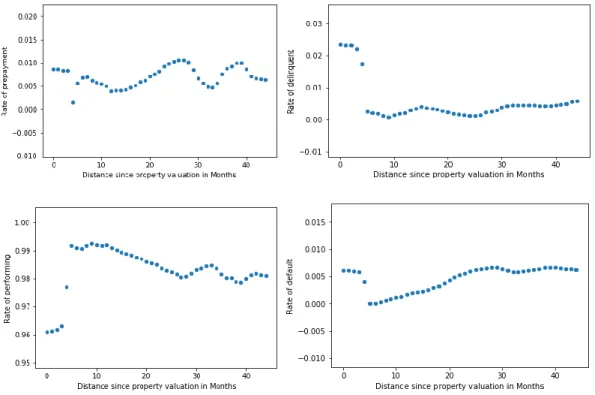
Looking, first of all, at the distance since property valuation, one can notice a very intense effect of time in first 5 months. The two graphs below illustrate this effect on the performing rate and the delinquent rate:

Figure 6

Here a significant shock can be seen, which intensity and direction were not expected (one would expect performing rates to decline and delinquency rate to increase over time). After which the recurring trends return (decline with time for performing rate and increase in time for delinquency rate). This effect has shown consistent when tested Sample 2 (Appendix B – figure 25). Moreover, this shock can also be distinguished by its singularity. It was not found in either the relationship between the distance since original property valuation and the loan states’ rate, nor in the

relationship between the loan states and time. On the contrary, much different effects are visible for these two variables, as illustrated by the graph below:

34

Figure 7

Looking at the relationship between time and performing rate, one can even observe an opposite effect at the same time with less intensity. This effect has also proven to be consistent when tested in Sample 2 (Appendix B – Figure 33). As for the relationships between the distance since original valuation and the loan states, together with the relationship between time and delinquency rate, one can see an effect happening much later with a smaller intensity. Consequently, the consistency of this intense effect, together with its singularity when compared to other related time interval factors suggest that it may not simply be noise in our data sample. It therefore carries relevant

information for our neural network’s input.

Holistically, we noticed these time intervals between different valuation and evaluation events have their own relationship with the loan states, either linear or non-linear, which appeared to be consistent in most cases when tested in Sample 2. We therefore concluded that they should be included in our model as the information they bring is relevant.

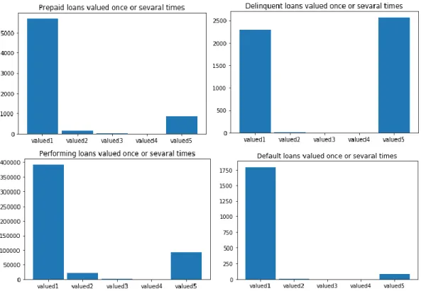
35 3.2.3 Number of valuations per Loan

The group also created a variable counting the number of times the loan has been valued. We wanted to assess whether trends could be observed between loans valued several times and a particular state. The combination done to create this variable was the following:

𝑁𝑢𝑚𝑏𝑒𝑟 𝑜𝑓 𝑣𝑎𝑙𝑢𝑎𝑡𝑖𝑜𝑛 𝑝𝑒𝑟 𝑙𝑜𝑎𝑛 = 𝑐𝑜𝑢𝑛𝑡 𝑜𝑓𝑣𝑎𝑙𝑢𝑎𝑡𝑖𝑜𝑛 𝑑𝑎𝑡𝑒 𝑝𝑒𝑟 𝑙𝑜𝑎𝑛

▪ called ValuationVolatility in the python notebook

Loans were valued from one to five times, the vast majority of them were valued once (see Appendix B – figure 34). No major trends were found, other than loans valued several times, if not classified performing, tended to be delinquent (Appendix B – figure 36).

3.2.4 Loan Age and related variables – FILIPE E HENRIQUE

The mortgage time path is quite important to understand the probability of a default or a prepayment. Three variables were created, in order to capture this effect of the mortgage track history in the probability of each state.

For each observation, we obtained the Loan Age which is the age of the mortgage, in months, the Distance to maturity, which gives the number of months until maturity and the Percentage of Loan Completion, which measures the loan’s age as a percentage of its length.

𝐿𝑜𝑎𝑛𝐴𝑔𝑒 = 𝑇𝑜𝑑𝑎𝑦’𝑠 𝑑𝑎𝑡𝑒(𝑌𝑟𝑀)– 𝐿𝑜𝑎𝑛𝑂𝑟𝑖𝑔𝑖𝑛𝑎𝑡𝑖𝑜𝑛𝐷𝑎𝑡𝑒 𝐷𝑖𝑠𝑡𝑎𝑛𝑐𝑒𝑇𝑜𝑀𝑎𝑡𝑢𝑟𝑖𝑡𝑦 = 𝐷𝑎𝑡𝑒𝑂𝑓𝐿𝑜𝑎𝑛𝑀𝑎𝑡𝑢𝑟𝑖𝑡𝑦 − 𝑇𝑜𝑑𝑎𝑦’𝑠 𝑑𝑎𝑡𝑒

% 𝑜𝑓 𝐿𝑜𝑎𝑛 𝐶𝑜𝑚𝑝𝑙𝑒𝑡𝑖𝑜𝑛 = 𝐿𝑜𝑎𝑛𝐴𝑔𝑒

(𝐷𝑎𝑡𝑒𝑂𝑓𝐿𝑜𝑎𝑛𝑀𝑎𝑡𝑢𝑟𝑖𝑡𝑦 − 𝐿𝑜𝑎𝑛𝑂𝑟𝑖𝑔𝑖𝑛𝑎𝑡𝑖𝑜𝑛𝐷𝑎𝑡𝑒)

Loan age, in particular, is one of the commonly studied determinants. For instance, the survival analysis, explained in section 1.2.3, bases its entire framework on the age of

36 the mortgage when there is a change in its state, computing a time conditional probability.

Some studies documented a positive effect of mortgage age in the probabilities of default, delinquency and prepayment; and a negative effect of mortgage’s age

squared in the three referred probabilities (Campbell, Tim S., and J. Kimball Dietrich; 1983). This paper, even though it is quite old, also shows that excluding the age-related variables from the regressions generates poorer model performance (less significance), than when we include them, what proofs the importance of the loan age in explaining

the states’ probabilities.

Most of the studies documented a non-linear relationship between mortgage’s

age and probabilities of default and prepayment. (Von Furstenberg, 1969), but specially

for default rates. In fact, “defaults display a rise-then-fall pattern as mortgage age”, in

the first years of the mortgage, it is common to have low default rates; as the time passes, the default frequency increase; however, it decreases again when the mortgage gets closer to its maturity.

Analyzing our sample, we can see a behavior between the both patterns, evidenced in the aforementioned literature.

In respect to default rate, we can see an approximation to the non-linear quadratic pattern described in literature, especially in the right tail, i.e., for older loans. Mortgages younger than 50 months and older than 250 months have a default rate close to zero; while ages between 50 and 250 months have default rates around 0.5%. For prepayment it is not so obvious, but the rate seems to be lower for loans older than 200 months (right tail), as expected, form literature; however, there is not a lower prepayment rate for younger loans. Loans younger than 200 months seem to have prepayment rates between 1 and 2%.

For performing and delinquent rates, the outcome is expected, although not extensively developed in related literature. Performing and delinquency rates follow the previous non-linear behavior, with a more prominent effect in older loans, like prepayment rate pattern. Delinquency seems to have a diminishing in older mortgages, while Performing has an upward trend.

37

Figure 8

The distance to maturity is the opposite of loan age. Young mortgages have high distance to maturity, while old mortgages are closer to maturity (low distance). We seek

to analyze how the proximity to each loan’s maturity dates influence the probability of

them defaulting or getting pre-paid. Therefore, this variable tries to capture how the

borrower’s decision is influenced by his mortgage’s proximity to termination.

The expected behavior should be similar of what happens in Loan Age: Mortgages too far or too close from maturity will have lower probabilities of being prepaid or defaulted, than mortgages with intermediate distances to maturity. At the beginning of the loan there are less incentives to prepay or default. Over time, there is a higher probability of a change in financial situation (positive or negative) that leads the borrower to delay, miss payments or to pay installments sooner, increasing the probability of a default or prepayment. Closer to maturity, the incentives to repay the mortgage sooner or stop paying it are lower, again.

Overall, from our in-sample behaviors for the four states the patterns are not as evident as Loan Age outcomes, however it can be observed the right tailor evidence as