Managing Capital Market and Longevity Risks in a Defined Benefit Pension Plan

(1)

DigitalCommons@University of Nebraska - Lincoln

Management Department Faculty Publications Management Department

9-2013

Managing Capital Market and Longevity Risks in a Defined Benefit

Pension Plan

Samuel H. Cox

University of Manitoba, [email protected]

Yijia Lin

University of Nebraska–Lincoln, [email protected]

Ruilin Tian

North Dakota State University, [email protected]

Jifeng Yu

University of Nebraska–Lincoln, [email protected]

Follow this and additional works at: https://digitalcommons.unl.edu/managementfacpub

Cox, Samuel H.; Lin, Yijia; Tian, Ruilin; and Yu, Jifeng, "Managing Capital Market and Longevity Risks in a Defined Benefit Pension Plan" (2013). Management Department Faculty Publications. 104.

https://digitalcommons.unl.edu/managementfacpub/104

This Article is brought to you for free and open access by the Management Department at

DigitalCommons@University of Nebraska - Lincoln. It has been accepted for inclusion in Management Department Faculty Publications by an authorized administrator of DigitalCommons@University of Nebraska - Lincoln.

(2)

Published online April 10, 2013.

Managing Capital Market and Longevity Risks

in a Defined Benefit Pension Plan

Samuel H. Cox, Yijia Lin, Ruilin Tian, and Jifeng Yu

Abstract

This article proposes a model for a defined benefit pension plan to minimize total funding variation while controlling expected total pension cost and funding downside risk throughout the life of a pension cohort. With this setup, we first investigate the plan’s optimal contribution and asset allocation strategies, given the projection of stochastic asset returns and random mortality evolutions. To manage longevity risk, the plan can use either the ground-up hedging strategy or the excess-risk hedging strategy. Our numerical examples demonstrate that the plan transfers more unexpected longevity risk with the excess-risk strategy due to its lower total hedge cost and more attractive structure.

Introduction

Operating defined benefit (DB) pension plans involves risks: no matter what happens in financial markets and how long employees live after retirement, DB plans are responsible for providing employees guaranteed retirement income. The inherent volatility of the capital market and longevity risk force the sponsors of the DB pension plans to manage pension risk.

The DB pension plans can reduce risk by pursuing a strategy with stable contributions (Lee, 1986). In this light, Haberman, Butt, and Megaloudi (2000) investigate an optimization

585

Samuel H. Cox is the L. A. H. Warren Chair Professor at the Asper School of Business, University of Manitoba. Yijia Lin is in the Department of Finance, College of Business Administration, University of Nebraska–Lincoln. Ruilin Tian is in the Department of Accounting, Finance, and Information System, College of Business, North Dakota State University. Jifeng Yu is in the Department of Management, College of Business Administration, University of Nebraska–Lincoln. The second author can be contacted via e-mail: [email protected]. This article was presented at the seventh International Longevity Risk and Capital Market Solutions Symposium in Frankfurt, Germany, in September 2011. The authors appreciate helpful comments from the participants at the meeting. The authors also thank the associate editor and the two anonymous referees for their very helpful suggestions and comments during the revision process.

(3)

problem with an objective to minimize the variance of periodic contributions. To cope with the risk, the sponsors can also adjust their asset allocation (Black, 1989; Bodie, 1991; Haberman, Butt, and Megaloudi, 2000; Colombo and Haberman, 2005; Maurer, Mitchell, and Rogalla, 2009; Lucas and Zeldes, 2009). A group of researchers is in favor of holding a 100 percent bond portfolio to minimize pension risk (Black, 1980; Gold and Hudson, 2003). The most prominent example of a company that follows this advice is the Boots, a U.K. pharmaceutical retailer, which shifted all of its pension assets to bonds between the spring of 2000 and July 2001.1 Yet, given that there exists a trade-off between contribution and the level of risk a DB scheme is willing to take (Colombo and Haberman, 2005), this practice may raise total pension cost as more contributions are needed to meet retirement benefit liabilities. Total pension cost includes all costs and penalties associated with normal contributions, supplementary contributions, and withdrawals (Maurer, Mitchell, and Rogalla, 2009). By contrast, some others advocate investing heavily in higher yielding but riskier equities, reasoning that stocks are expected to earn higher returns than bonds over the long haul and help to reduce underfunding over time. Still, there is a problem of this strategy. That is, equity investment increases funding variation and leads to a high funding downside risk, that is, the risk that pension assets fall far below pension liabilities. Thus, pension investment strategy should take into account both funding downside risk and total pension cost.

To derive the optimal proportion invested in risky assets, Maurer, Mitchell, and Rogalla (2009) minimize the variance of plan contributions subject to a total pension cost constraint but they do not explicitly control the plan’s funding downside risk. Delong, Gerrard, and Haberman (2008), on the other hand, investigate the optimal investment strategy by minimizing funding variation. While they include supplementary contributions in their generalized optimization problem, they do not directly study the effect of total pension cost on pension asset allocation. Josa-Fombellida and RincÓn-Zapatero (2004) also examine the pension asset allocation with the aim of minimizing pension funding risk and contribution rate risk, along the lines of Haberman and Sung (1994), Haberman (1997), and Josa-Fombellida and RincÓn-Zapatero (2001). They conclude that the plan will invest more in risky assets (e.g., stocks) when the funding status deteriorates. Bogentoft, Romeijn, and Uryasev (2001) model a multi-period problem to adjust contributions and investments at each decision point by minimizing pension cost subject to a conditional value at risk (CVaR) constraint on pension underfunding. Based on a pension fund data from the Netherlands, they suggest investing, on average, 84 percent of the pension fund in bonds and the remainder in equities. Similar to Delong, Gerrard, and Haberman (2008), Josa-Fombellida and RincÓn-Zapatero (2004) and Bogentoft, Romeijn, and Uryasev (2001) do not directly control total pension cost at a given level. Nevertheless, considering a total pension cost constraint is important since it includes all costs a plan incurs during a period of interest. The budget constraint creates a strong incentive for the plan to specify a target total pension cost.

To extend the previous analysis, in an asset–liability management setting with various stochastic assets and dynamic mortality rates, not only do we propose a problem to 1. However, the plan partially shifted back to equity investment in 2005.

(4)

minimize funding variation of a DB pension plan, but we also impose a constraint to specify expected total pension cost and a CVaR constraint to control downside risk from pension underfunding. We consider a financial market with a low-risk asset driven by a Brownian motion and each risky asset driven by a Lévy process. The dynamic mortality rates are described by the Lee and Carter (1992) model. Our model is straightforward and easy to implement.

Longevity risk has been recognized as a major threat to pension sponsors. Delong, Gerrard, and Haberman (2008) conclude that pension plans with higher longevity risk are subject to higher costs. We analyze how the optimal normal contribution and asset allocation will change with different levels of mortality improvement. Our numerical results show that given a funding downside risk tolerance, a higher life expectancy of pensioners leads to a higher optimal normal contribution and a higher percentage of funds invested in low-risk assets. In our example, when the common low-risk parameter in the Lee and Carter (1992) model decreases from –0.40 to x₀ (a more negative common risk parameter implies a higher level of mortality improvement), the expected total pension cost rises by 33 percent. To ensure the long-term financial health of pension plans, sponsors must find ways to mitigate longevity risk. The topic of longevity risk management of pension plans has attracted a great deal of attention in academics and industries (Lin and Cox, 2005, 2008; Blake et al., 2006; Cairns, Blake, and Dowd, 2006; Cox and Lin, 2007; Sherris and Wills, 2008; Brcic and Brisebois, 2010; Wills and Sherris, 2010). These authors discuss possible longevity risk management solutions such as plan design, annuity purchase, and longevity securities. We take this discussion one step further. Instead of just comparing and proposing different longevity hedging tools, we study how much longevity risk a plan should transfer. In particular, we add a longevity hedging element to our pension optimization problem. Given this setup, we solve for the plan’s optimal hedge ratio. Specifically, we look for optimal solutions for two longevity risk hedging strategies: the ground-up hedging strategy and the excess-risk hedging strategy. The ground-up hedging strategy transfers a proportion of all future retirement payments. A prominent example of the ground-up strategy is the EIB longevity bond offered in 2004. The excess-risk strategy is to cede the part of longevity risk that exceeds a given level. The 2008 survivor swap between Canada Life and owners of insurance-linked securities as well as other investors is based on this idea. Compared to the excess-risk hedging strategy, the ground-up strategy is more expensive and capital intensive. Our optimization results show that there exists a negative relation between hedge ratio and longevity hedge cost. Therefore, the plan tends to hedge much less with the ground-up hedging strategy. Our results offer a new explanation for the failure of the EIB bond. The approach is unique in that it describes how a longevity risk management strategy affects the magnitude of the plan’s hedge costs, which in turn determines its hedge level, whereas the earlier research on pension asset– liability optimization does not numerically analyze longevity risk transfer.

The article is organized as follows. The “Pension Fund Optimization” section describes the pension fund optimization model. We provide a numerical example to illustrate how to implement our model for a DB pension plan with a single cohort of employees. Then we

(5)

illustrate how longevity risk changes the optimal normal contribution and asset allocation. To hedge longevity risk, we examine the ground-up longevity risk hedging strategy in the section “Managing Pension Longevity Risks With the Ground-Up Hedging Strategy” The excess-risk hedging strategy has a lower cost than the ground-up hedging strategy. The section “Managing Pension Longevity Risks With the Excess-Risk Hedging Strategy” shows that the plan tends to hedge more unexpected risk with the excess-risk strategy. The results from the above-mentioned two sections provide important insights for longevity securitization, which is discussed in the “Implications for Longevity Securitization” section. The last section concludes the article.

Pension Fund Optimization

Basic Framework

Here we analyze a cohort whose members join a DB plan at the age of x₀ at time 0 and retire at the age of x at time T. We look for an optimal pension asset allocation and contribution strategy throughout the life of the cohort for the DB plan. In our setting, one period is a year. We further assume the cohort is stable across the entire accumulation phase. That is, every member who withdraws is replaced by a one at the same age.

In terms of the future curtate lifetime K(x) at age x, the present value of benefits of 1 per year is an annuity for K(x) years:

(1) where v = 1/(1 + r) is the discount factor at the discount rate r.

The probability that a plan member age x at time T survives to age x + s at time T + s (and gets a benefit payment) given the mortality table at time T is denoted as _sp˜_x,T. These are random variables for s = 1, 2, …, which we will simulate later. Define the conditional expected s-year survival rate for age x at retirement T as

This allows us to compute the conditional expected value of life annuity in (1) as

(2) That is, the life annuity factor for age x at retirement T, a(x(T)), is the discounted conditional expected value of payments of 1 per year as long as the retiree survives. This conditional expected value depends on future survival rates _sp˜_x,T, which are random variables viewed from time 0 because we are considering the mortality table to be random whereas in practice it is an estimate of future rates.

(6)

We can similarly define the life annuity factor for a retiree age y. After retirement T, the life annuity factor for age y (y > x) at time t (t > T), a(y(T)), is determined as:

(3) Here _spˆ_y,t is the conditional expected s-year survival rate for age y at time t,

where _sp˜_y,t is the probability that the retiree age y at time t survives to age y + s (and gets a benefit payment).

Suppose the plan starts with an accumulated fund PA₀ = M at time 0, which is invested in different assets. The value of the accumulated fund PA_t at time t depends on the amount invested in asset i at time t – 1, A_i,t_–1, and its return in period t, r_i,t :

(4) Regulations require the following balance equation to hold:

(5) where _{t – T}pˆ_x,Tis the conditional expected probability that a plan member age x at time T survives t – T years when t > T,

The normal contribution (or the normal cost) C represents new benefits earned by active participants each year. Following Haberman, Butt, and Megaloudi (2000), Maurer, Mitchell, and Rogalla (2009), and others, we assume the plan is free to choose a fixed normal contribution to minimize the variability of annual contributions. This means during the accumulation phase (t ≤ T), the sum of all investments at t, Σn_i₌₁A_i,t, equals the accumulated fund PA_t plus a constant normal contribution C (to be determined by optimization in the later sections) and a supplementary contribution k ∙ UL_t, where k is

the pension amortization factor and UL_t is the plan’s unfunded liability at time t. After retirement (t > T), the available fund for investment at time t is reduced by the benefits paid to the survivors, B ∙ _t_–_Tpˆ_x,T , where the constant B is the promised annual survival payment after the plan participants reach retirement age x at time T. It depends on the number of pensionable service years accrued until T and projected salaries before retirement.

(7)

We assume that regulations allow the plan to amortize the unfunded liability over m > 1 periods at the plan’s periodic discount rate ρ. This approach is common; see, for example, Maurer, Mitchell, and Rogalla (2009).2_{Therefore, the pension amortization factor}_k_equals

where

(6)

Following the literature, when t ≤ T, the plan’s unfunded liability UL_tequals

(7) When t > T, UL_t equals

(8) In (7) and (8), the pension liability at time t, PBO_t, is defined as the discounted value of future benefit obligations,

(9) In (9), the valuation rate ρ is set at a level reflecting the plan’s expectation on pension asset investment returns and future inflows of supplementary contribution (Delong, Gerrard, and Haberman, 2008).

2. Following Maurer, Mitchell, and Rogalla (2009), we assume pension shortfall has the same amortization period as surplus.

(8)

Equations (4) and (5) imply that the total fund available for investment at time t ≤ T, Σn_i₌₁ A_i,t, can be expressed as

(10) When t > T, Σn_i₌₁A_i,t becomes

(11) Assume the plan sponsor invests a proportion w_iof pension funds in asset i, i = 1, 2, …, n. The value of asset i at time t is

(12) When t = 0, A_i_,0 = w_iM for i = 1, 2, …, n.

The plan makes periodic contributions to meet future benefit obligations. Those contributions constitute the plan’s total pension cost. Following Maurer, Mitchell, and Rogalla (2009), we define total pension cost TPC as the present value of all normal contributions C, supplementary contributions SC_t, and withdrawals W_t:

(13) where

(9)

and

W_t = max {–k ∙ UL_t, 0}

The constants ψ₁ and ψ₂ are penalty factors on supplementary contributions SC_t and withdrawals W_t, respectively. The penalty factor ψ₁ accounts for the opportunity cost the plan sponsor incurs due to unexpected mandatory supplementary contributions SC_t that

could have been invested in positive net present value projects. And ψ₂ takes into account the tax benefits the plan forgoes when it reduces the plan’s normal contribution.

Objective Function and Optimization Problem

In our setting, the decision is taken at t = 0 and the plan accumulates assets and asset returns plus contributions less liability cash flows at t = 1, 2, … until the final age of the lives. Following Colombo and Haberman (2005) and others, we consider a pension plan that aims at minimizing funding variation. Consistent with much of the DB pension literature, we model this risk with a quadratic objective function J and measure supplementary contributions k ∙ UL_t using the spread method for underfunding amortization in (66):

(14) This objective function is similar to Colombo and Haberman (2005) who minimize the variance of the two-tail funding status. As a departure, Kouwenberg (2001) defines the risk of a pension plan as the average squared one-tail underfundings (i.e., only penalizing supplementary contributions but not withdrawals) across the accumulation phase. However, as pointed out by Haberman and Sung (2005), an excessive solvency surplus held in the pension fund can be expensive because overfundings increase opportunity costs from forgone profitable investment opportunities and taxes on nondeductible surplus and contributions. Thus, in practice, the plan tries to avoid both over- and underfundings. The “two-tail” objective function in (14) is consistent with this goal.

We also impose three constraints respectively to control the total pension cost defined in (13), the expected total unfunded liability E(TUL) , and the downside risk of the total unfunded liability up to the terminal age of the retirees. The total unfunded liability up to the terminal age of the retirees, TUL, is defined as

To manage the downside risk of the total unfunded liability, following Bogentoft, Romeijn, and Uryasev (2001), we include a CVaR constraint on TUL at some percentile of interest , denoted as CVar_(TUL).

(10)

Our optimization problem is to solve for the asset weights w = [w₁, w₂, …, w_n] and the normal contribution C, so as to minimize the funding variation J throughout the whole life of the cohort:

Minimize w, C subject to

(15) Different from Chang, Tzeng, and Miao (2003) who construct a weighted-average objective function that incorporates the first and second moments of underfunding, we impose the constraint E(TUL) = 0 and minimize the total funding variation. The E(TUL) = 0 constraint is also included in Delong, Gerrard, and Haberman (2008), Josa-Fombellida and Rincón-Zapatero (2004), and others. In (15) the expected total pension cost E(TPC) equals a preset target level ζ. The constant τ specifies the upper limit of the -level CVaR constraint on TUL. The constraint w_i ≥ 0 implies short-selling is not allowed.

As a robustness check, we compare our proposed model (15) with two alternative models, called problem (16) and problem (17), to investigate whether (15) can better balance funding variation, total pension cost, and funding downside risk. Problem (16) is to minimize E(TPC) subject to the E(TUL) and CVar_(TUL) constraints:

Minimize w, C subject to

(16) The objective function of (16) is similar to that in Bogentoft, Romeijn, and Uryasev (2001) who minimize the total cost of funding a pension plan.

(11)

Our second alternative model uses the same objective function as Haberman, Butt, and Megaloudi (2000) who define a weighted average function that addresses both funding variation and contribution rate risk. Specifically, their objective function is specified as:

(17) where θ is a weighting factor to reflect the relative importance of the funding variation risk against the contribution rate risk. The contribution cash flow mismatch (i.e., the contribution rate risk), CR_t, is defined as

(18) Here, C_tis the plan’s contribution at time t, t ≤ T. Specifically, C_tcan be decomposed into two parts based on the normal contribution C and the plan’s underfunding UL_tat time t, t ≤ T:

(19) Based on the objective function (17), our second alternative model has the same constraints as model (15). In Haberman, Butt, and Megaloudi (2000), the pension amortization factor k is a choice variable. In the United States, in some cases, the pension firms do not have any leeway to flexibly determine their pension amortization period.3_{Therefore, we do not} solve optimization problem (17) with respect to k.

In the “Optimization Results” section, we will use a numerical example to compare our proposed model (problem (15)) with its alternatives (problem (16) and problem (17)). The results show that problem (15) and problem (17) realize the same optimal solutions when the amortization period of unfunded liabilities is fixed. Problem (16) achieves a lower E(TPC) than problem (15) but is at the expense of a higher funding variation. As discussed earlier, managing total pension cost, funding variation, and funding downside risk in an integrated way is important for the plan. Thus, in this article we rely on optimization problem (15), the model with a more holistic view, to perform further analysis.

3. For example, in Franzoni and Marin (2006), “According to accounting regulations, if a loss emerges in a pension plan as a consequence of reduced assets or increased liabilities and the loss is larger than 10 percent of the maximum between the two items, then the company is obliged to amortize the loss starting from the next fiscal year. According to SFAS 87, the amortization period will be the average remaining service period of active employees expected to receive benefits under the plan. If all, or almost all, of a plan’s participants are inactive, the average remaining life expectancy of the inactive participants will be used instead of average remaining service.”

(12)

Example

Here we present a numerical example to show how to obtain the optimal normal contribution and asset allocation by solving optimization problem (15). We consider a cohort, all joining the plan at age x₀ = 45 at t = 0, and retiring at T = 20 when they reach age x = 65. We estimate that the benefit payment rate is c and number of survivors at age x is n,

so that B = nc = $10 million. The plan will pay benefits to survivors at times T + 1, T + 2, . . . so for each of the n retirees, the present value of benefits is c · a(x(T)), and the aggregate present value is the sum of n independent identically distributed benefits nc · a(x(T)) = 10

· a(x(T)) million at time T.

We assume the initial pension fund is M = $5 million at t = 0. The pension funds are invested in three assets: S&P 500 index A_1,_t, Merrill Lynch corporate bond index A_2,_t, and 3-month T-bill A_3,_t, with rates of returns r1,t_,_r

2,t, and r3,tin period t, respectively. The plan sets the

pension valuation rate at ρ = 0.08 and the life annuity factor discount rate at r = 0.05. It will amortize the unfunded liability over m = 7 years. Moreover, following Maurer, Mitchell, and Rogalla (2009) we assume the penalty factors on supplementary contributions and withdrawals are both equal to ψ₁ = ψ₂ = 0.2.

To model pension assets and mortality dynamics, we consider a probability space (Ω, F, F, P) with the filtration F = (F_t)_{0 ≤}_t_{≤ ∞}, where F_t is the information available up to

time t. The filtration F, denoted as F = FF _FM_{, consists of two subfiltrations where}_FF

contains information about the financial market and FM _{contains information about the}

mortality evolution. We assume the two subfiltrations FF_andM_{are independent. That is,}

the stochastic processes for assets and for mortality rates are independent.

Financial Market Model

We describe the process of the S&P 500 index at time t, A_1,_t, as the combination of a Brownian motion and a compound Poisson process as follows:

dA1,t

{

1 dt + σ1 dW1t, if the Poisson event does not occur at time t; A1,t = (1 − λ1k1) dt + σ1 dW1t+ (Y1 − 1), if the Poisson event occurs at time t.

(20) The constant ₁ is the drift of the S&P 500 index; σ₁ is its instantaneous volatility, conditional on no jumps. W₁_tis a standard Brownian motion with mean 0 and variance t. λ₁ is the mean number of arrivals per unit time of a Poisson process N1_t. The Poisson random measure N1_t counts the number of jumps of a particular size (Y₁ − 1) during a time interval of (0, t). A dramatic change (or a jump) in the value of S&P 500 index can be driven by the events such as the stock market downturn of 2002 or the recent financial crisis in the late 2000s. The Poisson process N1_t and the standard Brownian motion W₁_tare independent.

The parameter k₁ is k₁ ≡ E(Y₁ − 1), where E(Y₁ − 1) is the expected percentage change in the S&P 500 index if a Poisson event occurs.

The S&P 500 index, A_1,_t, will be continuous most of the time with finite jumps occurring at discrete points of time. The part “σ₁ dW₁_t” describes the instantaneous part of an

(13)

unanticipated “normal” S&P index change, and “Y₁ − 1” captures the “abnormal” shocks. If λ₁ = 0, then Y₁ − 1 = 0 and it is the same as the standard stochastic model without jumps. If ₁, σ₁, λ₁, and k₁ are constants, we can solve the differential equation (20) as

(21) The cumulative jump size Y(N1_t ) = 1 if N1_t = 0 and Y(N1_t ) = ∏N1t

j=1 Y1 jfor N1t ≥ 1,

where the jump sizes, Y₁_jfor j = 1, 2 . . ., are independent and identically distributed as lognormal random variables so that log Y₁_jis a standard normal random variable with mean parameter m₁ and volatility parameter s₁.

From (21), we can derive the S&P 500 index value A₁,_t_+Δ, given F_tresulting in

(22) where F_tis the information set up to time t.

Similarly, the Merrill Lynch corporate bond index A_2,_t_+Δgiven F_t is defined as follows: (23) where ₂ is the drift of the Merrill Lynch corporate bond index; σ₂ is the instantaneous volatility, conditional on no jumps. W₂_t is a standard Brownian motion with mean 0 and variance t. The jump sizes are independent lognormal random variables with parameters m₂ and s₂. The jumps Y₁_jand Y₂_iare independent for all i and j. The covariance of W₁_tand W₂_tis

Cov(W₁_t,W₂_t) = ρ₁₂ σ₁ σ₂t (24) where ρ₁₂ is the parameter measuring the dependence of the stock and bond indices. In addition, we assume the 3-month T-bill evolves according to a geometric Brownian motion as follows:

dA3,t

A_3,_t = 3 dt + σ3 dW3t (25)

where ₃, σ₃, and W₃_tare the drift, volatility, and standard Brownian motion of the 3-month T-bill. The differential equation (25) can be solved as

(14)

We further assume the 3-month T-bill is uncorrelated with the S&P 500 index and the Merrill Lynch corporate bond index,

Cov(W₁_t,W₃_t) = 0, and Cov(W₂_t,W₃_t) = 0.

We estimate models (22), (23), and (26) based on monthly data from March 1988 to December 2010. For the S&P 500 index and the Merrill Lynch corporate bond index, we rely on the time series data provided by DataStream. The monthly 3-month T-bill rates are obtained from FRED at Federal Reserve Bank of St. Louis.4_{We use the monthly data to increase the} number of observations for model calibration. Since we are interested in annual returns, we convert our monthly maximum likelihood estimates to annual estimates. Those annual estimates are presented in Table 1.

Table 1 indicates that the S&P 500 index has a higher expected log return (₁ = 0.1081) and volatility (σ₁ = 0.1069) than the Merrill Lynch corporate bond index (₂ = 0.0794, σ₂ = 0.0481) and the 3-month T-bill (₃ = 0.0523, σ₃ = 0.0094). The expected number of jumps per year for the stock index is λ₁ = 0.2946. For the corporate bond index the expected number of jumps per year is λ₂ = 0.0080 . Given a jump event occurs, the expected logarithm of the jump size is m₁ = −0.0272 for the stock index and m₂ = −0.0744 for the bond index. In addition, the stock index and the corporate bond index are positively correlated with correlation

parameter ρ₁₂ = 0.3380.

Stochastic Mortality Model. We apply the Lee and Carter (1992) model to describe pension mortality rates. This model incorporates both the age-specific mortality variation and the general time trend of mortality evolution for all ages. In this form of the Lee– Carter model, the logarithm of the 1-year death rate q_x_,_tat age x (x = 0, 1, 2, . . .) in year t (t = 1, 2, . . . , K) is

ln q_x_,_t= a_x+ b_xγ_t+ ε_x_,_t (27) where a_xand b_xare the age-specific parameters.

The transitory shock ε_x_,_t is a normally distributed variable with zero mean. The time series common risk factor γ_taffects the mortality rates of all ages in year t. Lee and Carter (1992)

Table 1. Maximum Likelihood Parameter Estimates of Three Pension Assets

Parameter Estimate Parameter Estimate Parameter Estimate

₁ 0.1081 ₂ 0.0794 ₃ 0.0523 σ₁ 0.1069 σ₂ 0.0481 σ₃ 0.0094 λ₁ 0.2946 λ₂ 0.0080 m₁ −0.0272 m₂ −0.0744 s₁ 0.0536 s₂ 0.0000 ρ₁₂ 0.3380 4. http://research.stlouisfed.org

(15)

assume γ_tfollows a random walk with drift g,

γ_t= γ_t₋₁ + g + e_t (28) where the error term e_tis normally distributed with a zero mean and a variance σ_γ. The solution of (27) is not unique so the following two constraints are imposed:

∑ bx = 1 and ∑ γ_t= 0 (29)

x t

These two constraints imply that the intercept a_xis simply the empirical average of age x over time:

K

a_x= ∑t=1 ln qx,t (30) K

where K is the length of the time series of mortality data. We follow the Lee and Carter’s (1992) method by incorporating singular value decomposition to estimate b_xfor each age x and γ_tfor each year t.

We assume the pension plan has the same mortality experience as that of the U.S. male population and it estimates model (27) following the Lee and Carter (1992) procedure. The tables for years 1901 to 1999 are from the Human Life Table Database and the tables for 2000 to 2007 are from the Human Mortality Database, published by the University of California, Berkeley, and Max Planck Institute for Demographic Research.5_{The estimated}

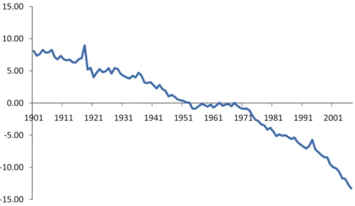
γ_tare shown in Figure 1.6 Based on the ages x = 0, 1, 2, . . ., and the time series of γ_twhere t = 1901, 1902, . . . , 2006, 2007, we obtain g = −0.20 and σ_γ= 0.63 for (28).

Now consider a cohort who joins the plan at age x₀ = 45 in year 2007. After setting year 2007 as the base year t = 0, we forecast the mortality rates q₄₅₊_t_,_tfor t = 1, . . . , T, T + 1, . . . . We first simulate the error term e_tand then add the constant g = −0.20 to each simulated e_tto get a γ_twhere t = 1, 2, . . . , T, T + 1, . . . . Given the estimated a₄₅₊_t’s and b₄₅₊_t’s and the simulated γ_t’s, we use model (27) to calculate simulated future mortality rates

˜

q₄₅₊_t_,_t= ea45+t + b45+t γt +ε45+t,t, t = 1, 2, . . . , T, T + 1, . . . .

The forecasted 1-year survival probability is

˜

p₄₅₊_t_,_t = 1 − q˜₄₅₊_t_,_t

5. Available at http://www.mortality.org or http://www.humanmortality.de (data downloaded on February 25, 2011).

(16)

This pension cohort will retire at time t = T = 20 when all pensioners reach age x = 45 + t = 65. Based on the simulated survival rates forecasted with the Lee–Carter model, we calculate the conditional expected value of the life annuity a(x(T)) using (2):

(31) where

After retirement T, we use (3) to determine the value of the life annuity a(y(t)) for y > x =

65 and t > T = 20,

(32) where

Figure 1. Estimated Time Series Common Risk Factor γ_t Shown in the Vertical Axis for Year t = 1901, 1902, . . . , 2006, 2007 in the Horizontal Axis.

(17)

With the values of a(x(T)) and a(y(t)), the value of the pension liability PBO_tat time t, t = 0, 1, … can be calculated from (9).

Optimization Results. We set year 2007 as the base year t = 0 and ran a Monte Carlo simulation with 1,000 iterations to generate returns for three financial assets A_i_,_t i = 1, 2, 3 and future liabilities PBO_tfor t = 1, 2, . . . .7_{Initially, we assume the plan invests equally} in the three assets, that is, w₁ = w₂ = w₃ = 1_/_{3 and makes an annual normal contribution}_C = 1. This strategy leads to an expected total pension cost E(TPC) = 15.01. As shown in the row labeled “Initial” in Table 2, the initial strategy has a 95 percent CVaR of TUL equal to CVaR_95%(TUL) = 69.66 and an expected TUL equal to E(TUL) = 3.79. The sum of all funding variations throughout the whole lives of the pension cohort equals J = 984.20.

Next we solve the optimization problem (15) to obtain the optimal asset allocation and normal contribution. Based on our experiments, given the same ζ = 15.01 as the E(TPC) of the initial case, we find that the lowest feasible upper limit of CVaR_95%(TUL) for (15) equals τ = 59.63. With the combination of ζ = 15.01 and τ = 59.63, the optimal solution for (15) is shown in the row labeled “Problem (15)” in Table 2. To achieve the lowest funding variation, on average, the plan should invest w₁ = 17.13 percent of the funds in the S&P 500 index, w₂ = 69.82 percent in the Merrill Lynch corporate bond index, and the remaining funds should be invested in the 3-month T-bill with w₃ = 13.06 percent. In addition, given E(TUL) = 0, the optimal normal contribution equalsC = $1.07 million per year.Our optimization problem (15) achieves E(TUL) = 0 and it has a lower funding downside risk CVaR_95%(TUL) = 59.63 and a lower total funding variation J = 935.63 than the initial case with CVaR_95%(TUL) = 69.66 and J = 984.20.

Our results show that problem (17) with different θs has the same optimal asset allocation and normal contribution as our proposed model (15) shown in Table 2. This is not surprising because when UL_t > 0, the supplementary contribution SC_t equals k · UL_tand when UL_t < 0, the plan has a withdrawal W_t= −k · UL_t. That is, UL_tdetermines the deviation of the actual periodic contribution C_tfrom the normal contribution C in (19). In fact, when the

Table 2. Model Comparison

C w₁ w₂ w₃ E(TPC) CVaR_95%(TUL) E(TUL) J Initial 1.00 33.33% 33.33% 33.33% 15.01 69.66 3.79 984.20 Problem (15) 1.07 17.13% 69.82% 13.06% 15.01 59.63 0.00 935.63 Problem (16) 1.06 21.16% 61.40% 17.45% 14.90 59.63 0.00 942.57

7. In our numerical example we only consider three assets but our model can handle a higher number of assets.

(18)

pension amortization factor k is specified at a given level, the objective function of problem (17) can be restated as:

(33) which is the same as the objective function of problem (15) scaled by a constant (θ + (1 −

θ)k2_{). This explains why problem (15) and problem (17) have the same solution and our} setting is equivalent to Haberman, Butt, and Megaloudi (2000) when k is a constant. Finally, we compare problem (16) with problem (15). To make comparison comparable, we set the constraints in (16),

E(TUL) =0 and CVaR_95%(TUL) ≤ 59.63,

which are the same as those in our example for (15). Table 2 shows that problem (16) has a little lower E(TPC) but a higher total funding variation J than problem (15). This can be explained by the fact that problem (16) aims at minimizing E(TPC) but does not manage the total funding variation. Since both funding variation and downside risk are the major concerns for pension risk management, in the following discussion, we focus on problem (15) that takes a more balanced view.

Longevity Risks

Mortality has improved over time. The example in the “Stochastic Mortality Model” section, which we call the base case, shows that on average the value of the common risk factor γ_tdecreases by 0.20 across all ages per year from 1901 to 2007 (i.e., g = −0.20). However, the tendency of pension participants to live longer than what the historical data suggest has been increasingly attracting the attention of plan sponsors, regulators, actuaries, academics, and others. This is so-called longevity risk, the risk that the mortality of pensioners improves at a higher rate than expectation. Accordingly, an interesting question for the pension plan is: if the mortality improves more than the base case with g =

−0.20, how will it change the optimal asset allocation and normal contribution?

In particular, we consider mortality dynamics under which the pension liability is an increasing function of survival probabilities, as higher survival probabilities will yield a longer lifetime and a longer duration of annuity payments. In a sensitivity analysis of the plan’s total pension cost to the longevity risk, we change the drift of the common risk

factor γ_tin the Lee and Carter (1992) model in an equal interval of 0.05 from the base case g = −0.20 to g = −0.40. A more negative g means a greater level of mortality improvement.

(19)

Next, given a level of funding downside risk, we investigate how the optimal normal contribution, asset allocation, and total pension cost will change with the life expectancy of pensioners. Specifically, we solve a problem that minimizes

_T₂ J = E

[

∑

(

ULt

)

]

t=1_{(1 +}_ρ₎t

subject to the constraint E(TUL) = 0 and a 95 percent CVaR constraint on total unfunded liability, CVaR95%(TUL). To make our comparison comparable, we specify this CVaR constraint as

CVaR_95%(TUL) = 59.63,

which ensures the unexpected mortality improvement cases with different gs have the same downside risk as the base case with g = −0.20.

Notice we do not impose the constraint E(TPC) = ζ when we examine longevity risk effects due to regulatory considerations. Theoretically, as pensioners live longer, to achieve a target expected total pension cost E(TPC), the pension plan has to make less normal contribution and invest a higher proportion of funds in risky assets (Josa-Fombellida and Rincón-Zapatero, 2004). However, in reality, regulators will not allow an underfunded plan to reduce its contribution and speculate on risky assets simply to realize a target E(TPC). Instead, E(TPC) has to be adjusted upward to reflect a higher longevity risk as shown in Table 3.

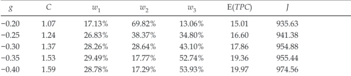
In Table 3, the adverse effect of an unexpected mortality improvement is captured by the change in E(TPC) paid by the plan. As g decreases from −0.20 to −0.40, E(TPC) significantly increases from 15.01 to 19.97, a 33 percent rise. In addition, we observe a higher life expectancy of the pensioners (with a more negative g) leads to a higher optimal normal contribution: C increases from 1.07 with g = −0.20 to 1.59 with g = −0.40. Also notice that as the mortality improves, the plan needs to invest more in the low-risk asset to satisfy the downside risk constraint CVaR_95%(TUL) = 59.63. The proportion of total funds invested in the 3-month T-bill dramatically increases from 13.06 percent with g = −0.20 to 53.93 percent with g = −0.40.

Table 3. Optimal Pension Normal Contribution and Asset Allocation Strategies With E(TUL) = 0 and CVaR_95%(TUL) = 59.63 and Different Assumptions on Mortality Improvement Parameter g in the Lee and Carter (1992) Model.

g C w₁ w₂ w₃ E(TPC) J −0.20 1.07 17.13% 69.82% 13.06% 15.01 935.63 −0.25 1.24 26.83% 38.37% 34.80% 16.60 941.38 −0.30 1.37 28.26% 28.64% 43.10% 17.86 954.88 −0.35 1.53 29.49% 17.77% 52.74% 19.36 955.44 −0.40 1.59 28.78% 17.29% 53.93% 19.97 974.56

(20)

It is difficult for a plan to predict future mortality rates. The resulting uncertainty can immediately affect the stability of the pension plan through, at least, wrong asset allocations and inappropriate normal contributions. However, if the pension plan can hedge its longevity risk, it will suffer much less from financial distress due to unexpected mortality improvement. Therefore, we turn our attention to analyzing optimal hedging decisions. In the next two sections, we discuss two pension longevity risk hedging strategies: the ground-up hedging strategy and the excess-risk hedging strategy.

Managing Pension Longevity Risks with the Ground-Up Hedging Strategy

In this section, we study the optimal hedging decision for a pension plan when it implements the ground-up hedging strategy. This strategy transfers a proportion hG_of

the pension liability, represented by the shaded area hG_Ba₍_x₍_T_{)) in Figure 2, to a hedge}

provider where 0 ≤ hG_{≤ 1. The hedge provider will pay a proportion}_hG_{of benefits due to}

retirees at time T + 1, T + 2, . . . .

Specifically, let E[Ba(x(T))] = B a¯(x(T)). At time t = 0, the pension plan starts with an accumulated fund M and cedes a portion hG_{of the plan liability}_Ba₍_x₍_T_{)) to a third party}

(e.g., longevity-security investors), who accepts the obligation for a price equal to8 HPG₌hG (1 + δG)B a¯(x(T))

(1 + ρ)T

where δG_{is the unit hedge cost. The unit hedge cost}_δG_{covers risk premium, issuance cost,}

and administrative expenses of the longevity risk taker as well as the time and resources

Figure 2. The Ground-Up Hedging Strategy; Ba(x(T ))max_{Stands for the Highest Possible Pension} Liability Ba(x(T )); This Strategy Hedges a Proportion hG_{(0 ≤ h}G_{≤ 1) of the Pension Liability Ba(x(T )),}

Represented by the Shaded Area hG_{Ba(x(T ))}

8. In our article, the price HPG_{for the ground-up strategy (or HP}E_{for the excess-risk strategy) is the}

market price determined by the capital market. We assume the plan takes the price HPG _{(or HP}E₎

as given for its optimal hedging decision. An example of HPG_{is the annuity premium General}

(21)

the plan spends to transfer its longevity risk. As a result, the pension plan retains a liability of (1 − hG₎_PBOG

tand its liability at time t becomes

(34) Meanwhile, the plan invests in the capital market to generate investment income. Given that the plan hedges a fraction hG_{of its pension liability by paying}_HPG_{, the total amount}

of pension assets available for investment at t = 0 is PAG₀ = MG₌_M₋_HPG

which is lower than that in the no-hedge case where PA₀ = M. The balance equation under the ground-up hedging strategy changes to:

(35) The underfunding liability equals

(36) where PAG_tis the value of pension assets before the plan makes contributions and pays survival benefits at time t.

Similar to (10), the total fund available for investment at time t ≤ T, ∑n_i₌₁AG_i_,_tin (35) for the ground-up strategy equals

(37) When t > T, ∑n_i₌₁AG_i_,_t becomes

(22)

Assume the plan sponsor invests a proportion wG_iof pension funds in asset i, i = 1, 2, . . . , n. The value of asset i at time t is

(39) When t = 0, AG_i_,0 = w_i MG_for_i_{= 1, 2,}_{. . .}_,_n_.

The optimal investment and contribution policy is subject to a total pension cost constraint. Compared to the no-hedge case, the ground-up hedging strategy has an additional cost component—the hedge cost. For each dollar hedged, the plan pays δG_{dollars to set up the}

contract. After hedging hG_Ba₍_x₍_T_{)) of the plan liability, the plan pays a total pension cost}

with the present value at time 0 equal to:

(40) where hG_δG_B_a_¯₍_x₍_T₎₎_/_{(1 +}_ρ₎T_{is the present value of the total hedge cost.}

How to Transfer Longevity Risk with the Ground-Up Hedging Strategy?

The optimization problem of the pension plan with respect to the asset weights wG_{= [}_w 1

G_, w₂G, …, w_nG], normal contribution CG_{, and hedge ratio}_hG_{is expressed as:}

Minimize

(23)

where TULG_{= ∑∞} t=1 ULG_t . The constraint (1 + ρ) t hG_{(1 +}_δG₎_B_¯_a₍_x₍_T₎₎ ≤ M (1 + ρ)T

ensures the hedge price does not exceed the pension fund at t = 0. That is, the plan does not borrow money to pay for the cost of risk transferred.

Example

Here we continue the example in the previous “Example” section, but now assume that the plan implements a ground-up hedging strategy.We set E(TPC) and the upper bound of CVaR_(TUL) at the same levels as those in the optimal case without hedging (see the row labeled “Problem (15)” in Table 2). The results are shown in Table 4. When hedging is costless (δG_{= 0), subject to the total pension cost constraint}_ζ_{= 15}_._{01 and the upper limit}

of the TUL 95 percent CVaR constraint τ = 59.63, the plan hedges 21 percent of the pension liability. This allows the plan to achieve a total funding variation

which is lower than that in the no-hedge case J G_{= 935}_._{63 when}_hG_{= 0.}

When the plan hedges, it incurs an explicit cost and an implicit cost. The explicit cost is the unit hedge cost δG_{. The implicit cost arises from the reduced fund available for investment}

since the fund available for investment decreases from M to MG_{. The plan sacrifices a}

higher expected return from the risky asset class in exchange for a lower longevity risk. However, longevity risk hedging is attractive only if its benefits exceed costs. Table 4 shows a negative relation between the hedge ratio hG_{and the unit hedge cost}_δG_{. The plan}

chooses to hedge less as hedging becomes more expensive. As δG_{increases from 0 to 0.03,}

the hedge ratio hG_{decreases from 21 to 1 percent. When}_δG_{goes above 0.03, no longevity} Table 4. Optimal Ground-Up Hedging Strategies with Different Assumptions on Hedge Cost Parameter δG_Given_ζ_{= 15.01,}_τ_{= 59.63, and g= −0.20}

δG _CG _w 1 G _w 2 G _w 3 G _h_G _CVaR 95%(TULG) J G 0.000 1.09 19.37% 77.87% 2.76% 21% 51.82 917.18 0.010 1.08 20.07% 76.89% 3.04% 21% 52.28 925.83 0.020 1.07 18.50% 74.80% 6.70% 13% 55.31 932.86 0.025 1.07 17.95% 72.33% 9.72% 7% 57.25 934.83 0.030 1.07 17.24% 69.96% 12.79% 1% 59.45 935.61 0.035 1.07 17.13% 69.82% 13.06% 0% 59.63 935.63

(24)

risk will be ceded. Moreover, as the hedge ratio hG_{goes down, the plan’s total funding}

variation J G_{increases due to, at least, higher longevity risk.}

Managing Pension Longevity Risks with the Excess-Risk Hedging Strategy

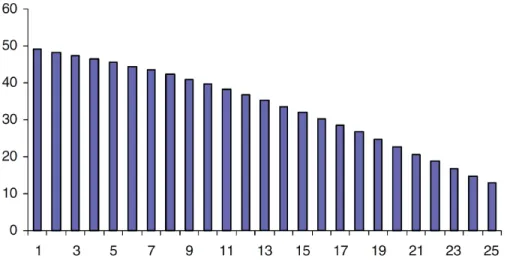
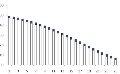
Although the ground-up hedging strategy in the “Managing Pension Longevity Risks with the Ground-Up Hedging Strategy” section reduces longevity risk, it has two major problems. First, it provides a protection that the plan may not need. The plan can predict its future payments to some extent and it is only uncertain about the amount exceeding its expectation. The cost of hedging is usually proportional to the amount of coverage. As such, the ground-up strategy is expensive. In addition, this strategy is capital intensive. It requires a large up-front premium, which the plan may not afford. The first longevity bond, the EIB bond issued in November 2004, is an example of the ground-up hedging strategy. It is a 25-year bond that provides a protection equal to the amount of a fixed annuity, £50 million, multiplied by the percentage of the reference population still alive at each anniversary. The coverage of this bond is illustrated as the solid filled bars in Figure 3. The EIB bond offered a hedge to pension plans but the EIB did not sell. The ground-up protection structure, at least partially, explains its failure (Lin and Cox, 2008). A more attractive structure is the one that only covers the annuity payment that exceeds a certain strike level. The modified EIB bond we suggest is shown in Figure 4. The unfilled area of each bar in Figure 4 represents the risk retained by the plan. The plan only cedes the longevity risk above the strike levels, which are represented as the solid filled bars. This illustrates the second strategy we examine in this section: the excess-risk hedging strategy.

Figure 3. Coverage of the EIB Longevity Bond. Note: The solid filled bars show the protection provided by the EIB longevity bond each year (millions in pounds); the horizontal axis represents time in years.

(25)

With the excess-risk strategy, the plan needs to determine a threshold level for each of the years T + 1, T + 2, … above which to transfer a proportion hE_{of risk. Recall that the}

conditional expected s-year survival rate, _spˆ_x_,_T, for age x at retirement T is defined as,

spˆx,T= E[sp˜x,T|p˜x,T, p˜x+1,T+1, … , p˜x+s–1,T+s–1],

which is random at time 0. Suppose at time 0, the plan transfers the risk that exceeds the plan’s expectation, _s¯p_x_,_T= E[_spˆ_x_,_T], after the plan participants reach the retirement age x at time T,

max[B _spˆ_x_,_T− B _s¯p_x_,_T, 0] s = 1, 2, …, (42) which can be viewed as a set of European call options written at time 0 and exercised

at T + 1, T + 2, …. In this example, the strike price equals the expected survival benefit, B_s¯p_x_,_T, s = 1, 2, …. Of course, the plan can set a different threshold given its risk tolerance, for example, one or two standard deviations above the mean B_s¯p_x_,_T, s = 1, 2, …. In the “Optimization with a Different Strike Level“ section, we investigate how a change in the strike level will change the optimal hedging strategies. Because the excess-risk strategy only cedes the high-end risk, in general, it has a much lower capital requirement for the protection than the ground-up strategy.

Figure 4. Coverage of the Modified EIB Longevity Bond Using the Excess-Risk Hedging Strategy. The solid filled bars show the protection provided by the excess-risk hedging strategy each year (millions in pounds) and time in years is on the horizontal axis.

(26)

If the plan hedges a proportion hE_{of (42), it needs to pay a price equal to}

HPE₌h

E_{(1 +}_δE_{) E}

[

_{∑ ∞}

s=1vsmax[Bspˆx,T − Bs ¯px,T, 0]

]

(1 + ρ)T

where δE_{is the hedge cost per dollar hedged in the excess-risk hedging strategy and}

E

[

∑ ∞_s₌₁vs_max[_B

spˆx,T − Bs ¯px,T, 0]

]

is the present value of expected payments from the longevity risk taker at time T. As such, the plan’s liability at the end of period t becomes

(43) After the plan buys the excess-risk longevity hedge, the fund ME_{it can invest in the capital}

market at t = 0 is

ME₌_M₋_HPE

The excess-risk hedging strategy should satisfy the following balance equation:

(44) In (44), the underfunding liability in the excess-risk strategy equals

(45) where PAE_tis the value of pension assets at time t before the plan makes contributions and pays survival benefits at time t.

(27)

From (44) and (45), the total fund available for investment at time t ≤ T, ∑n_i₌₁AE i,t can be written as (46) When t > T, ∑n_i₌₁AE i,t is calculated as: (47) Therefore, the value of asset i at time t given the weight wE_i is

(48) When t = 0, AE

i,0 = wi MEfor i = 1, 2, . . . , n.

The excess-risk strategy has a total pension cost TPCE_{as follows:}

(49) where hE_δE_E

[

_{∑ ∞}

s=1vsmax[Bspˆx,T − Bs ¯px,T, 0]

]

/(1 + ρ)T is the total hedge cost. Recall that TPCG_{in (40) is the total pension cost of the ground-up hedging strategy. Both}_TPCG_and TPCE _{have a hedge cost component. However, the hedge cost components of these two}

strategies are not equal due to different hedging structures and possibly different unit hedge costs (δG_vs._δE_{). This can lead to very different optimal hedging solutions for these}

(28)

How to Manage Longevity Risks With the Excess-Risk Hedging Strategy?

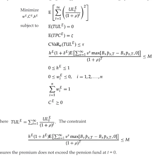
The optimal excess-risk hedging strategy is to solve the following optimization problem: Minimize

subject to

(50) where The constraint

ensures the premium does not exceed the pension fund at t = 0.

Example

Continue the example as in the section mentioned initially. This time the plan adopts the excess-risk hedging strategy with the strike level B_s¯p_x_,_T, s = 1, 2, . . . and T = 20. It solves problem (50) to obtain the optimal normal contributionCE , the asset allocations wE_i(i = 1, 2, 3), and hedge ratio hE_{that will minimize the total funding variation,}

subject to E(TULE_{) = 0, E(}_TPCE_{) =}_ζ_{= 15}_._{01, and CVaR}

95%(TULE) ≤ τ = 59.63.

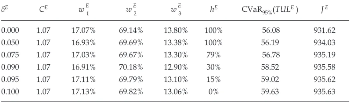
Table 5 summarizes the results with different unit hedge costs δE_{. As long as}_δE _{is not}

(29)

hE_>_{0. In these cases, the total funding variations}_J E_{are all lower than the case without}

hedging longevity risk. However, the hedging will not do anything good when δE_{≥ 0}_._{10 so}

the plan chooses to retain all risks (hE_{= 0 percent).}

The hedge ratios hE_{in Table 5 are much higher than}_hG_{for the ground-up hedging in Table}

4, which creates an apparent contrast between the excess-risk strategy and the ground-up strategy. This can be explained by the more attractive structure and the lower capital requirement of the excess-risk strategy. The excess risk strategy only covers the payment above the strike level. However, the ground-up strategy covers the entire risk, including the payment the plan can predict reasonably. As such, the ground-up strategy requires a higher price that reflects the higher future payments from the hedge provider. This means the plan has to give up a large proportion of the initial fund M and forgo possibly higher returns from the capital market. In this case the plan decides to hedge less. Moreover, the hedge cost increases with the amount of coverage. The unneeded coverage provided by the ground-up strategy increases the hedge cost. This further discourages the plan from hedging with the ground-up strategy. In contrast, the excess-risk strategy focuses on the protection the plan really needs. In our example, as long as the unit hedge cost is not too high (δE_{≤ 0}_._{05), the plan will hedge all of the excess longevity risk.}

One must use caution when comparing the total funding variation J G_{in Table 4 with}_J E_in

Table 5. One might find it striking that many values of J E in Table 5 are higher than those of J G_{in Table 4 and then might conclude that the excess-risk strategy retains a higher extreme}

longevity risk. This may not be true because this belief does not recognize that the total funding variation reflects not only longevity risk, but also investment risk. Actually, the higher variation J E_{in the excess-risk strategy arises from the higher amount available for}

asset investments (i.e., ME_{> M}G_{). In our example, the expected annuity payment}_B_¯_a₍_x₍_T₎₎

equals $110.13 million and the expected excess-risk payment is

= $1.34 million.

Table 5. Optimal Excess-Risk Hedging Strategies With Different Assumptions on Hedge Cost Parameter δE_Given_ζ_{= 15.01,}_τ_{= 59.63, g= −0.20, and the Strike Level B}

s¯px,T , s = 1, 2, . . . and T = 20 δE _CE _wE 1 w E 2 w E 3 hE CVaR95%(TULE ) J E 0.000 1.07 17.07% 69.14% 13.80% 100% 56.08 931.62 0.050 1.07 16.93% 69.69% 13.38% 100% 56.19 934.03 0.075 1.07 17.03% 69.67% 13.30% 79% 56.78 935.19 0.090 1.07 16.91% 70.18% 12.90% 30% 58.52 935.58 0.095 1.07 17.11% 69.79% 13.10% 15% 59.02 935.62 0.100 1.07 17.13% 69.82% 13.06% 0% 59.63 935.63

(30)

Assuming δG₌_δE_{= 0, the price of the ground-up hedging strategy paid to the risk taker}

at t = 0 is

$4.96 million, while the price of the excess-risk strategy is only

$0.29 million.

This implies that the initial fund available for asset investment in the ground-up strategy is

PAG₀ = MG_{= 5 − 4}_._{96 = $0}_._{04 million,}

which is much lower than that in the excess-risk strategy PAE₀ = ME_{= 5 − 0}_._{29 = $4}_._{71 million}_.

Since the risky assets’ volatility, in general, is much higher than that of longevity risk, we observe a higher funding variation of the excess-risk strategy. Nevertheless, the excess-risk strategy has a much lower high-end longevity risk than the ground-up strategy as hE_{> h}G

for all cases when δE = δG < 0.10 as illustrated in this example.

Discussion of Asset Allocations With and Without Hedging. In our article, we follow a common assumption in the pension literature that the stochastic processes for assets and mortality are independent.9_{With this setting, the main driver of the interaction between} investment risk and longevity risk is the hedge price paid to the longevity risk taker. After a plan sets its target expected total pension cost and downside risk level, the hedge price the plan pays for the ceded risk determines the amount available for asset investments that in turn affects asset allocation. In our example, to achieve the lowest funding variation without hedging, on average, the plan should invest 17.13 percent of the funds in the S&P 500 index, 69.82 percent in the Merrill Lynch corporate bond index, and the remaining funds should be invested in the 3-month T-bill with 13.06 percent as shown earlier in Table 2 and reproduced for comparison in Table 6.