Received November 15th, 2017, 1st Revision May 15th, 2018, 2nd Revision September 14th, 2018, Accepted for publication October 24th, 2018.
Copyright © 2018 Published by ITB Journal Publisher, ISSN: 2337-5787, DOI: 10.5614/itbj.ict.res.appl.2018.12.3.2
Performance Comparison of LEACH and LEACH-C
Protocols in Wireless Sensor Networks
Ala’a Al-Shaikh*, Hebatallah Khattab & Saleh Al-SharaehDepartment of Computer Science, King Abdulla II School for Information Technology, University of Jordan, Amman, Jordan
*E-mail: [email protected]
Abstract. Wireless Sensor Networks (WSNs) draw the attention of researchers due to the diversity of applications that use them. Basically, a WSN comprises many sensor nodes that are supplied with power by means of a small battery installed in the node itself; the node can also be self-charged by a solar cell. Sometimes it is impossible to change the power supply of battery-operated nodes. This dictates that sensor nodes must utilize the energy they have in an optimal manner. Data communication is the main cause of energy dissipation. In this context, designing protocols for WSNs demands more attention to the design of energy-efficient routing protocols that allow communications between sensor nodes and their base station (BS) with the least cost. LEACH is a prominent hierarchical cluster-based routing protocol. It groups sensor nodes into clusters to reduce energy dissipation. On the other hand, LEACH-C is a protocol based on LEACH that claims to improve energy dissipation over LEACH. In this paper, a successful attempt was made to compare these two protocols using MATLAB. The results show that LEACH-C has better performance than LEACH in terms of power dissipation.
Keywords: energy-efficient protocols; LEACH; LEACH-C; protocol comparison; routing protocols; wireless sensor networks.
1
Introduction
A wireless sensor network (WSN) comprises sensors that are spatially distributed [1] and deployed in an area called the sensor field [2]. Each sensor collects data and sends it to a central aggregation unit known as the base station (BS) or sink [3]. WSNs have a wide spectrum of applications, including environmental monitoring, target tracking, healthcare monitoring, and machine automation [1, 4, 5].
Sensor nodes are low-cost electronic devices equipped with sensors, microprocessors, memory, wireless transceivers, batteries, and low-power GPS devices [6]. The basic components of a sensor node are shown in Figure 1. The sensors are limited in power, storage, and range [3]. They can perform: (1)
computation, (2) communication, and (3) sensing [1]. Basically, they connect to each other via a wireless medium and collaborate to perform a certain task [7].
Figure 1 Basic components of a sensor node [8].
Mainly, sensors are not equipped with energy backup, which makes them one-time-use sensors [9]. In addition, WSNs have limited battery life, which makes energy-efficiency the most important factor [10] to consider when planning to extend network lifetime [11]. Depending on the type of application, WSNs are either operated for a given operation time, or they can be put into service until their sensor nodes totally die [12].
Low-energy adaptive clustering hierarchy (LEACH) is the most fundamental, energy-efficient cluster-based protocol for WSNs and is used to reduce power consumption [13,14]. Meanwhile, LEACH-C is a centralized cluster-based routing protocol [14].
In this paper, we consider some parameters to compare the LEACH and LEACH-C protocols. We used MATLAB to simulate two WSNs, one that uses LEACH and one that uses LEACH-C as their routing protocols. Based on the results obtained by running the simulation, a comparison was made. The remainder of this paper is organized as follows: in Section 2 related work is reviewed. Then the methodology used in this study is shown in Section 3. Some necessary background is presented in Section 4. Our work is presented in Section 5, which contains the experimental settings and results. Finally, the paper is concluded in Section 6.
2
Related Work
Nayak & Shree [13] used NetSim simulator to compare LEACH and LEACH-C to verify the properties of both. They used several performance metrics, such as total number of data signals delivered at the BS over time, average energy dissipation over time, location of BS vs average energy dissipation, and location
of the BS vs lifetime of network. According to the results they obtained, they concluded that LEACH-C performed better than LEACH.
Geetha, et al. compared the LEACH and LEACH-C protocols using NS-2 [14]. They chose different scenarios and measured several performance metrics; their main concern was latency and network lifetime. They concluded that LEACH-C provides increased network lifetime and the desired number of clusters.
In a similar work conducted by Xinhua & Sheng [15], the authors compared the performance of the LEACH and LEACH-C protocols using the NS-2 simulator. Their main concern was to find a method to find out the effective factor in the comparison between the two protocols. They focused on the location of the sink and tested whether location affects the performance of the protocols or not. According to the results obtained, the authors concluded that neither protocol is superior to the other and it is not possible to recommend one protocol for a specific scenario or application. Additionally, a proper selection between both protocols is key to extending WSN life.
An improved version of both LEACH and LEACH-C protocols was introduced by Zhao, et al. [16]. The new protocol not only improves the selection process of the cluster heads in response to the change of the amount of node energy. The proposed protocol also assigns a vice cluster head for each cluster in an attempt to reduce the energy consumed and extend WSN lifetime. A simulation of the proposed protocol was conducted using NS-2, comparing it to LEACH and LEACH-C using the following three parameters: (1) number of nodes alive over the time of the experiment, (2) amount of energy consumed over the time of the experiment, and (3) amount of messages created by each protocol. According to the authors, the proposed protocols, i.e. the improved protocols, showed better performance than both LEACH and LEACH-C in terms of energy consumption, which results in longer WSN lifetime.
In a more comprehensive work, Omari & Fateh [17] compared six protocols, three of them based on the LEACH protocol and the other three based on the HEED protocol. Using MATLAB, the protocols were implemented and evaluated based on the following parameters: (1) number of control packets, (2) number of rounds, (3) live nodes, (4) data delivery to the base station, and (5) the residual energy in each round. The authors concluded that the LEACH family of protocols offers better performance than the HEED family of protocols.
3
Methodology
The LEACH and LEACH-C algorithms were implemented in MATLAB. At the beginning of the simulation, some parameters were we set. Both protocols require a number of rounds; after the desired number of rounds is finished, the results are collected and analyzed. Charts are depicted according to the results and then illustrations and explanations of the results are made. Finally, our results were compared to some similar work in the literature.
4
Background
4.1
LEACH and LEACH-C
Nodes that are within the transmission range of each other can communicate directly without the need for a routing protocol. On the other hand, nodes that are not within the range of each other, e.g. nodes A and C in Figure 2, need to send data to an intermediate node, e.g. B in Figure 2, which will forward packet forward and backward since it overlaps the transmission ranges of both nodes A and C.
Figure 2 A number of nodes and their ranges in a WSN [18].
Direct communication between nodes can take place when: (1) the nodes are neighbors, and (2) when the nodes have large enough transmission power. Nevertheless, this could be a drawback because of the large amount of energy required to establish high transmission power [12]. Routing protocols can be classified into: (1) flat protocols in which there are no master or referential nodes, and (2) hierarchical protocols in which some nodes are assigned some superior tasks over others [19]. Figure 3 shows a cluster-based hierarchical model of a WSN. This network comprises several clusters, also known as clumps, where each has its own cluster head (CH), which is responsible for data
transmission to all sensors in that cluster [13]. Nodes that are not cluster heads are called cluster members (CMs) [2]. Intra-cluster and inter-cluster coordination are the responsibility of CHs [21]. By intra-cluster coordination we mean the coordination between nodes within the same cluster and the aggregation of their data. On the other hand, inter-cluster coordination is the communication between CHs themselves or communications between CHs and BSs [21]. In other words, CHs carry out communication between CMs, while BSs carry out communications between CHs [2].
Figure 3 Cluster-based hierarchical model [20].
The number of CHs has an influence on the energy consumption. If a WSN contains many CHs, the energy consumption generated by communications between the CHs and the BS will be increased. Also, if the WSN contains a small number of CHs, the energy consumption generated by data aggregation and communication between CMs and CHs will be increased [22]. Low energy adaptive clustering hierarchy (LEACH) is the most fundamental hierarchical protocol (cluster-based protocol), which is the base of most of the existing energy efficient protocols [23]. Clustering in LEACH is illustrated in Figure 3 [20]. LEACH performs a number of rounds, each consisting of two phases, the set-up phase and the steady-state phase [22, 23] as follows:
1. Set-up phase: in this phase, CHs are randomly selected to collect and
aggregate data from sensors in clusters and eventually transmit results to BSs [22]. A node becomes a CH by randomly selecting a number between 0 and 1 [23]. If this number is smaller than a predefined threshold, then this node becomes a CH for the current round. Afterwards, the CH is determined and advertises its status. Then, the remaining nodes select their CHs by sending join-request messages depending on the strength of the received signal of the advertisement signals [20,22]. Then, the selected CH applies a time division multiple access (TDMA) schedule to the cluster
group members to organize the sending of the messages to the CH and then to the base station [24]. Figure 4 illustrates this phase using a flowchart.
Figure 4 Flowchart of the set-up phase of the LEACH protocol [24].
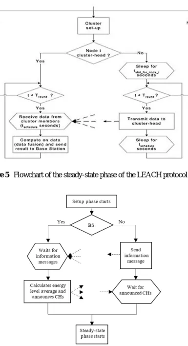
2. Steady-state phase: this is the phase in which the WSN performs its
intended tasks by aggregating data and transferring them to the BS (sink) [12,20]. When the clusters are established and the TDMA schedule is announced, the process of data transmission can be started. Each non-cluster-head node that has data to transfer, sends its data to the CH during its allocated transmission time. To save energy in the non-cluster-head nodes, their radio is turned off until their allocated transmission time starts. On the other hand, the CH must keep its receiver on to be always ready to receive any data from the cluster nodes. When CH receives all data, it executes signal processing functions to create a composite single signal and sends it to the base station [24]. The steady-state phase is illustrated in Figure 5.
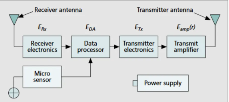
However, in order not to drain the battery of some nodes, especially those that are selected as CHs, LEACH randomly rotates CH positions and thus extends their lifetime [25]. LEACH-Centralized (LEACH-C) uses a centralized clustering algorithm to select CHs in the set-up phase. Instead of randomly selecting CHs, all nodes of WSN send their information, which are their current locations and energy levels, to the BS. After that, the BS computes the average level of the energy of all nodes. Any node that has energy more than the calculated average will have a chance to be a cluster head. When the BS
receives the information sent by the nodes and calculates the average energy, it decides which nodes will be CHs and advertises that to the whole WSN [27,28]. Figure 6 shows the flowchart of the LEACH-C set-up phase.
Figure 5 Flowchart of the steady-state phase of the LEACH protocol [26].
The steady-state phase is performed the same way as in the LEACH protocol. This modification of LEACH represented by the LEACH-C protocol is intended to prolong WSN lifetime and lower energy dissipation [13].The BS receives the location data from the nodes, decides which nodes to select as CHs, and advertises that to the whole WSN [27]. In LEACH-C, nodes with an energy level greater than a predetermined threshold, i.e. the average energy level calculated by the BS, are selected to be CH by the BS [29,14]. This modification of LEACH represented by the LEACH-C protocol prolongs WSN lifetime and lowers energy dissipation [13].
Unlike in LEACH, where each node has the chance to become a CH in different rounds, not all the nodes in LEACH-C will have the same chance [29]. One of the major drawbacks of LEACH-C when compared to LEACH is that it suffers increased energy dissipation during the set-up phase due to the initial communication between the BS and the nodes, which results in more data reception at the BS [13,27].
4.2
The Energy Model
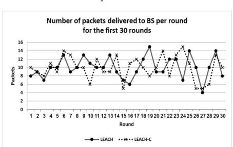
Figure 7 shows the energy dissipated in each component of the sensor node.
Figure 7 The energy cost associated with each component of the sensor node [29].
In Figure 7, only components that are incorporated in the communication process are shown. The communication device component of the sensor node shown in Figure 1 is further divided into receiver, transmitter, and amplifier to show the cost of energy incurred at each component. 𝐸𝑅𝑅 is the per-bit energy dissipated in reception and 𝐸𝑇𝑅 is the per-bit energy dissipated in transmission [29]. The data aggregation energy, which is defined as the energy dissipated in data processing (aggregation) is denoted by 𝐸𝐷𝐷 [29, 30]. The amplifier energy
𝐸𝑎𝑎𝑎(𝑟) is the energy required by the transmit amplifier to maintain an
acceptable signal-to-noise ratio in order to transfer data messages reliably [29]. For a message of length k bits, to travel from source to destination passing a distance d, the following two equations hold [29]:
𝐸𝑇(𝑘,𝑑) =𝑘 × (𝐸𝑇𝑅+𝐸𝑎𝑎𝑎(𝑑)) (1)
𝐸𝑅(𝑘) =𝑘×𝐸𝑅𝑅 (2)
Such that 𝐸𝑇(𝑘,𝑑) is the total energy dissipated in the transmitter of the source node to transmit a message of length 𝑘bits over a distance 𝑑, and 𝐸𝑅(𝑘) is the total energy dissipated in the receiver of the destination node to receive a message of length 𝑘 bits [29].
Amplification is calculated based on the channel model: a threshold value 𝑑𝑜 is calculated; if the distance is less than the threshold value then the free-space model is used, otherwise the multipath-fading model is used [26]. The amplifier incorporates the free space and multipath fading channel models each with a parameter, i.e. 𝜀𝑓𝑓 and 𝜀𝑎𝑎 respectively [26,29]. Based on these two parameters,
𝑑𝑜 can be calculated as follows: 𝑑𝑜 =�𝜀𝑓𝑓/𝜀𝑎𝑎 [23]. Accordingly, 𝐸𝑎𝑎𝑎(𝑑) is
given by Eq. (3) [26]: 𝐸𝑎𝑎𝑎(𝑑) =�𝜀𝑓𝑓𝑑 2, 𝑑 ≤ 𝑑 𝑜 𝜀𝑎𝑎𝑑4, 𝑑>𝑑𝑜 (3)
4.3
Simulation Tool
Many tools are available to simulate WSNs, each with different features, limitations, environments, and written in different programming languages. Some well-known tools are: (1) Network Simulator 2 (NS-2) [31], (2) Network Simulator 3 (NS-3) [32], (3) Matrix Laboratory (MATLAB) [33], and (4) Objective Modular Network Testbed in C++ (OMNeT++) [34].
In our work, we chose MATLAB to simulate the protocols under comparison depending on our review of the literature. For example, in [35] a survey was conducted to show the popularity of the tools mentioned above. The metric for the popularity of these tools was the number of papers published in international conferences and journals that used these tools. The results showed that NS-2 was the most used, followed by MATLAB. The advantages of MATLAB listed in [36] overcame those of NS-2. Besides, [37] points out the main drawbacks of NS-2 as a simulator of WSNs. One of them is the lack of a sensing model. Also, the used parameters of simulating the nodes in WSN as energy model, packet formats, and MAC protocols are totally different as they are used in real-world
sensor network scenarios. On the other hand, MATLAB is considered the base language for several simulators, such as PROWLER [38]. In addition, it is required for other tools to be installed such as PiccSIM [39]. Moreover, MATLAB is included as a toolbox in other simulators, for example LabVIEW [40]. Regarding the features of MATLAB, some of the most significant ones are the ease of programming capability and its possession of an easy platform that attracts users to develop their own functions. Furthermore, MATLAB has numerous toolboxes, such as Control System Design, Aerospace, Fuzzy Logic, Statistics, Symbolic Computations, Communication and several others, which encouraged us to use it in our work [36].
5
Experimental Settings and Results
5.1
Experimental Settings
In this paper, an attempt was done to compare between the aforementioned two hierarchical cluster-based protocols, LEACH and LEACH-C. MATLAB 7.6 R2008 A was used in the experiments. Table 1 summarizes the experimental settings used in this paper. These values were selected based on some tuning that was done until values were reached that could be read, recorded, and analyzed.
We assume a number of 100 nodes distributed in a 100x100 meters sensor area. Nodes were placed at random points, each had (x, y) coordinates. The BS (sink) was located at the center of the sensor field, i.e. at (50, 50).
Table 1 Summary of parameter settings.
Parameter Value
Number of nodes (N) 100 + 1 BS
Sensor field area 100x100
Node distribution Random
Number of rounds (𝑅𝑎𝑎𝑅) 500
Channel type Wireless
Communication channel Bidirectional
BS coordinates (50, 50)
Initial node energy (𝐸𝑜) 0.2J
CH probability (p) 0.1
Energy dissipation in reception (𝐸𝑅𝑅) 50 nJ/bit Energy dissipation in transmission (𝐸𝑇𝑅) 50 nJ/bit
Radio propagation model Free Space and Multipath Free-space amplifier parameter (𝜀𝑓𝑓) 10 pJ/bit/m2 Multipath amplifier parameter (𝜀𝑎𝑎) 0.0013 pJ/bit/m4
Basic operation of both protocols assumes having CHs and CMs; these are sometimes referred to as advanced and normal nodes respectively. The total number of nodes in the WSN is equal to the number of sensor nodes plus one sink (BS); this equals 101 nodes. The initial energy in each node was 0.2 J. As basic operation of LEACH selects a node to be CH based on a value between 0 and 1, this value was set to 0.1 in the experiment.
Furthermore, for the purposes of the experiment the following values were set:
𝐸𝑇𝑅 = 𝐸𝑅𝑅 = 50 𝑛𝑛/𝑏𝑏𝑏,ε𝑓𝑓 = 10 𝑝𝑛/𝑏𝑏𝑏/𝑚2, ε𝑎𝑎 = 0.0013 𝑝𝑛/𝑏𝑏𝑏/
𝑚4,𝑎𝑛𝑑𝐸
𝐷𝐷 = 5 𝑛𝑛/𝑏𝑏𝑏/𝑚𝑚𝑚𝑚𝑎𝑚𝑚. The simulation ran for 500 rounds
(𝑅𝑎𝑎𝑅 = 500).
It should be noted that although the number of rounds in the simulation was 500, only the first 30 rounds were included in most of the charts so they can be easily read and analyzed.
5.2
Results and Discussion
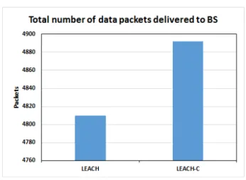
We start our discussions with the number of data packets delivered to the BS. Actually, this is a very important metric that can be used as evidence that supports our discussions of the lifetime of the WSN using both protocols. Figure 8 shows the number of data packets sent to the BS in the first 30 rounds.
Figure 8 Number of data packets sent to the BS.
Figure 9 shows the total number of data packets delivered to the BS for both the LEACH and C protocols. It is obvious from Figure 9 that the LEACH-C protocol could deliver more data packets to the BS compared to LEALEACH-CH.
Figure 9 Summary of the total number of data packets delivered to the BS.
In an attempt to give a more precise interpretation of the operations of the protocols, the rounds were grouped into chunks of 50 rounds each, as shown in Figure 10, so that we can gain a better understanding of the operations of the two protocols in terms of data packets.
Figure 10 Number of data packets sent to the BS grouped into 10 50-round chunks.
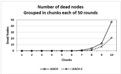
The chart in Figure 11 shows the total number of dead nodes in each round. The importance of Figure 11 is to illustrate the behavior of the nodes obtained in Figure 8. In Figure 8, the number of data packets delivered to the BS decreases over time. Figure 11 illustrates the reason in terms of dead nodes. In other words, the number of packets decreases due to the increase in the number of dead nodes, as shown in Figure 11.
Figure 11 Number of dead nodes grouped in chunks of 50 rounds each.
Starting from the 7th chunk, i.e. between the 301st to the 350th round, nodes in our configuration started to die. As the simulation makes more rounds, the number of dead nodes increases proportionally. Furthermore, in networks that use the LEACH protocol, nodes start dying earlier than the nodes of the networks that use the LEACH-C protocol, as is obvious from Figure 11. This supports the theoretical foundation that LEACH-C is an enhancement of the LEACH protocol to prolong lifetime of WSNs. Eventually, the number of dead nodes at the end of the 500 rounds was greater when using the LEACH protocol.
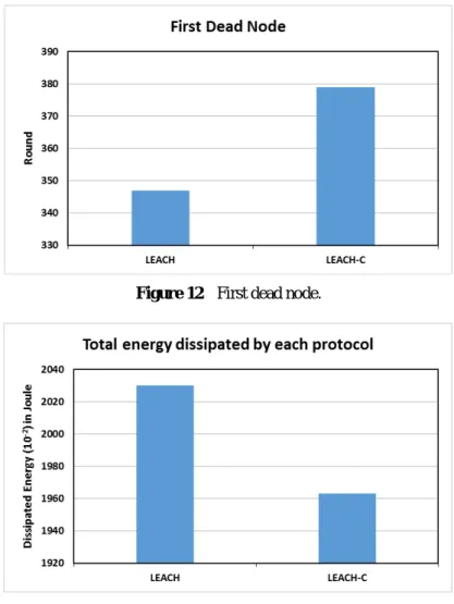
Back to Figure 9, which shows that the LEACH-C protocol could deliver more data packets to the BS than LEACH. The explanation for this is that using the LEACH from the 7th group of rounds, i.e. starting from round 350, nodes started to die due to the dissipation of their energy, as we saw already in Figure 11. Comparing that to the LEACH-C protocol, also starting from the 7th chunk of rounds, there were less dying nodes. Another metric we looked at in our results was the first dead node, which is shown in Figure 12. The first node dying took place earlier in LEACH than in LEACH-C. This is another important factor that supports the purpose of LEACH-C, which is designed to extend the lifetime of the network.
The most important factor any research has to look at in the study of WSN protocols is energy dissipation. Figure 13 shows the total energy dissipated by each protocol. Prolonging network lifetime could be done by consuming less energy at the sensing nodes that used the LEACH-C protocol than the nodes that used the LEACH protocol, as shown in Figure 13.
Figure 12 First dead node.
Figure 13 Total energy dissipated by each protocol.
Looking at Figure 14, it can be seen that starting from the 7th chunk, LEACH-C shows less energy dissipation than LEACH. Looking back at Figure 12, the first node died in LEACH in round 347, which is part of the 7th chunk. After more rounds, more nodes died, as we saw in Figure 11. This can be read in two directions: the more rounds we have, the more dead nodes we have due to more energy dissipation. Reversely, it can also be read as: the more rounds we have, the more energy dissipation we have and thus the more dead nodes exist. An important observation found in our exploration of the LEACH-C protocol is that there are some rounds when no nodes are selected to be CHs, i.e. CH count in a particular round is zero. Based on the operation of LEACH-C, CHs are
selected by the BS based on a threshold value: candidate nodes must have energy greater than that predetermined value. As the nodes’ energy dissipates during rounds of operation, there may be some rounds in which none of the nodes have remaining energy greater than the threshold value. The threshold value is adjusted to a level lower than the previous threshold value so that LEACH-C operation can continue.
Figure 14 Total energy dissipated grouped in chunks of 50 rounds each.
6
Conclusion
In this paper, an experiment was conducted based on a MATLAB simulation of a WSN to compare between two prominent energy-efficient protocols, LEACH and LEACH-C. Several performance metrics were observed. The most important among them is the energy dissipation metric due to the fact that the energy dissipation is crucial to the design of WSN protocols. Our findings fully comply with the theory: it was found that LEACH dissipated more energy than LEACH-C, which gives LEACH-C an advantage over LEACH in that it prolongs WSN lifetime. The results obtained in this paper converge with other results obtained in the literature. This work can be used as a basis to compare more protocols with the LEACH protocol as long as LEACH is the fundamental protocol for hierarchical cluster-based WSN protocols.
References
[1] Gautam, G. & Sen, B., Design and Simulation of Wireless Sensor
Network in NS2, International Journal of Computer Applications,
[2] Ganeshkumar, P., Vijayakumar, K.P. & Anandaraj, M., A Novel Jammer
Detection Framework for Cluster-Based Wireless Sensor Networks,
EURASIP Journal on Wireless Communications and Networking, 2016
(1), Article No.35, 2016.
[3] Fahim, H., Javaid, N., Khan, Z.A., Qasim, U., Javed, S., Hayat, A., Iqbal, Z. & Rehman, G., Bio-inspired Routing in Wireless Sensor Networks, in 2015 9th International Conference on Innovative Mobile and Internet Services in Ubiquitous Computing (IMIS), 2015 .
[4] Bhalla, M., Pandey, N. & Kumar, B., Security Protocols for Wireless
Sensor Networks, in 2015 International Conference on Green Computing
and Internet of Things (ICGCIoT), 2015.
[5] Ferng, H-W., Tendean, R. & Kurniawan, A., Energy-Efficient Routing Protocol for Wireless Sensor Networks with Static Clustering and
Dynamic Structure, Wireless Personal Communications, 65(2), pp.
347-367, 2012.
[6] Mann, R.P., Namuduri, K.R. & Pendse, R., Energy-Aware Routing
Protocol for Ad Hoc Wireless Sensor Networks, EURASIP Journal on
Wireless Communications and Networking, 2005(5), pp. 635-644, 2005. [7] Mondal, R.K. & Sarddar, D., Data-Centric Routing Protocols in Wireless
Sensor Networks: A Survey, COMPUSOFT, An International Journal of
Advanced Computer Technology, 3(2), pp. 593-598, 2014.
[8] Manap, Z., Ali, B.M., Ng, C.K., Noordin, N.K. & Sali, A., A Review on
Hierarchical Routing Protocols for Wireless Sensor Networks, Wireless
Personal Communications, 72(2), pp. 1077-1104, 2013 .
[9] Cho,Y. & Jung, J., Virtual Protocol Stack for WSN Simulators, ACM SIGAPP Applied Computing Review, 11(1), pp. 7-13, 2010.
[10] Abrardo., Balucanti, L. & Mecocci, A., A Game Theory Distributed
Approach for Energy Optimization in WSNs, ACM Transactions on
Sensor Networks (TOSN), 9(4,) pp. 1-22, 2013.
[11] Singh, S.K., Singh, M.P. & Singh, D.K., Routing Protocols in Wireless
Sensor Networks – A Survey, International Journal of Computer Science
& Engineering Survey (IJCSES), 1(2), pp. 63-83, 2010.
[12] Saad, E., Awadalla, M. & Darwish, R., Adaptive and Energy-Efficient
Clustering Architecture for Dynamic Sensor Networks, International
Journal of Computers and Applications, 31(4), pp. 282-289, 2011.
[13] Nayak, P. & Shree, P., Comparison of Routing Protocols in WSN Using
NetSim Simulator: LEACH Vs LEACH-C, International Journal of
Computer Applications, 106(11), pp. 1-6, 2014 .
[14] Geetha, V., Kallapur, P. & Tellajeera, S., Clustering in Wireless Sensor Networks: Performance Comparison of LEACH & LEACH-C Protocols
Using NS2, in 2nd International Conference on Computer,
Communication, Control and Information Technology (C3IT-2012), 2012.
[15] Xinhua, W. & Sheng, W., Performance Comparison of LEACH and
LEACH-C Protocols by NS2, 2010 Ninth International Symposium on
Distributed Computing and Applications to Business, Engineering and Science, pp. 254-258, 2010.
[16] Zhao, F., Xu, Y. & Li, R., Improved LEACH Routing Communication
Protocol for a Wireless Sensor Network, International Journal of
Distributed Sensor Networks, 8(12), 2012.
[17] Omari, M. & Laroui, S., Simulation, Comparison and Analysis of Wireless Sensor Networks Protocols: LEACH, LEACH-C, LEACH-1R,
and HEED, 2015 4th International Conference on Electrical Engineering
(ICEE), 2015.
[18] Johnson, D.B. & Maltz, D.A., Dynamic Source Routing in Ad Hoc
Wireless Networks, in Mobile Computing, Kluwer Academic Publishers,
pp. 153-181, 1996.
[19] Biradar, R.V., Patil, V.C, Sawant, S.R. & Mudholkar, R.R., Classification and Comparison of Routing Protocols in Wireless Sensor
Networks, Special Issue on Ubiquitous Computing Security Systems, 4,
pp. 704-711, 2009.
[20] Sharma, N. & Verma, V., Heterogeneous LEACH Protocol for Wireless
Sensor Networks, Int. J. Advanced Networking and Applications, 5(1),
pp. 1825-1829, 2013.
[21] Younis, O. & Fahmy, S., HEED: A Hybrid, Energy-Efficient, Distributed
Clustering Approach for Ad Hoc Sensor Networks, IEEE Transactions on
Mobile Computing, 3(4), pp. 366-379, 2004.
[22] Kao, C.C., Yeh, C.N. & Lai, Y.T., Low-Energy Cluster Head Selection
for Clustering Communication Protocols in Wireless Sensor Network,
International Journal of Computers and Applications, 33(1), pp. 9-14, 2011.
[23] Pramanick, M., Chowdhury, C., Basak, P., Al-Mamun, M.A. & Neogy,
S., An Energy-Efficient Routing Protocol for Wireless Sensor Networks,
in 2015 Applications and Innovations in Mobile Computing (AIMoC), 2015.
[24] Panchal, S., Raval, G. & Pradhan, S.N., Optimization of Hierarchical
Routing Protocol for Wireless Sensor Networks with Identical Clustering,
International Conference on Advances in Communication, Network, and Computing, 2010.
[25] Heinzelman, W.R., Chandrakasan, A. & Balakrishnan, H.,
Energy-Efficient Communication Protocol for Wireless Microsensor Networks, in
2014 47th Hawaii International Conference on System Sciences, 2000. [26] Heinzelman, W.B., Chandrakasan, A. & Balakrishnan, H., An
Application-Specific Protocol Architecture for Wireless Microsensor
Networks, IEEE Transactions on Wireless Communications, 1(4), pp.
[27] Khediri, S.E., Nasria, N., Weic, A. & Kachourid, A., A New Approach for
Clustering in Wireless Sensors Networks Based on LEACH, Procedia
Computer Science, 32, pp. 1180-1185, 2014.
[28] Peng, Z.R., Yin, H., Dong, H.T. & Li, H., LEACH Protocol Based
Two-Level Clustering Algorithm, International Journal of Hybrid Information
Technology, 8(10), pp.15-26, 2015.
[29] Muruganathan, S.D., Ma, D.C.F., Bhasin, R.I. & Fapojuwo, A.O., A Centralized Energy-Efficient Routing Protocol for Wireless Sensor
Networks, IEEE Communications Magazine, 43(4), pp. S8-S13, 2005 .
[30] Sindhwani, N. & Vaid, R., V Leach: An Energy Efficient Communication
Protocol for WSN, Mechanica Confab, 2(2), pp. 79-84, 2013.
[31] Information Sciences Institute, The Network Simulator-ns2. Available from: http://www.isi.edu/nsnam/ns, retrieved on September 10th, 2018. [32] NSNAM Team, The Network Simulator-ns3. Available from:
http://www.nsnam.org/docs/release/3.14/tutorial/singlehtml/index.html, Retrieved on September 10th, 2018.
[33] MATLAB website www.mathworks.co, Retrieved on September 10th, 2018.
[34] Varga, A. & Hornig, R., An Overview of the Omnet++ Simulation
Environment, in Proceedings of the 1st International Conference On
Simulation Tools and Techniques for Communications, Networks and Systems & Workshops, ICST (Institute for Computer Sciences, Social-Informatics and Telecommunications Engineering), Article No. 60, 2008. [35] Tran, O., Kim, T., Nguyen, V.D. & Hong, C.S., Which Network
Simulation Tool is Better for Simulating Vehicular Ad-Hoc Network,
Proceedings of the Korean Information Science Society, 41, pp. 930-932, 2014.
[36] Nayyar, A. & Singh, R., A Comprehensive Review of Simulation Tools
for Wireless Sensor Networks (WSNs), Journal of Wireless Networking
and Communications, p-ISSN: 2167-7328 e-ISSN: 2167-7336, 5(1), pp.19-47, 2015.
[37] Singh, C.P., Vyas, O.P., & Tiwari, M.K., A Survey of Simulation in
Sensor Networks, in CIMCA '08 Proceedings of the 2008 IEEE
International Conference on Computational Intelligence for Modelling Control & Automation, pp. 867-872, 2008.
[38] Prowler Website http://www.isis.vanderbilt.edu/projects/nest/prowler/ , Retrieved on September 10th, 2018.Piccsim Website http://wsn.aalto.fi/ en/tools/piccsim/, Retrieved on September 10th, 2018.
[39] Labview Website: www.ni.com/labview/, Retrieved on September 10th, 2018.
![Figure 1 Basic components of a sensor node [8].](https://thumb-us.123doks.com/thumbv2/123dok_us/1697492.2735251/2.892.259.611.217.376/figure-basic-components-sensor-node.webp)
![Figure 2 A number of nodes and their ranges in a WSN [18].](https://thumb-us.123doks.com/thumbv2/123dok_us/1697492.2735251/4.892.273.596.555.750/figure-number-nodes-ranges-wsn.webp)
![Figure 3 Cluster-based hierarchical model [20].](https://thumb-us.123doks.com/thumbv2/123dok_us/1697492.2735251/5.892.256.626.341.562/figure-cluster-based-hierarchical-model.webp)
![Figure 4 Flowchart of the set-up phase of the LEACH protocol [24].](https://thumb-us.123doks.com/thumbv2/123dok_us/1697492.2735251/6.892.302.549.240.524/figure-flowchart-set-phase-leach-protocol.webp)