Cornell University School of Hotel Administration Cornell University School of Hotel Administration
The Scholarly Commons
The Scholarly Commons
Working Papers School of Hotel Administration Collection
11-2017
Option-Implied Systematic Disaster Concern
Option-Implied Systematic Disaster Concern
Fang Liu Ph.DCornell University School of Hotel Administration, [email protected]
Follow this and additional works at: https://scholarship.sha.cornell.edu/workingpapers Part of the Finance and Financial Management Commons
Recommended Citation Recommended Citation
Liu, F. (2017). Option-implied systematic disaster concern [Electronic version]. Retrieved [insert date], from Cornell University, School of Hotel Administration site: http://scholarship.sha.cornell.edu/ workingpapers/38
This Working Paper is brought to you for free and open access by the School of Hotel Administration Collection at The Scholarly Commons. It has been accepted for inclusion in Working Papers by an authorized administrator of The Scholarly Commons. For more information, please contact [email protected].
Option-Implied Systematic Disaster Concern
Option-Implied Systematic Disaster Concern
AbstractAbstract
The covariation of option-implied disaster concern of the market index and individual stocks allows me to estimate the conditional and systematic disaster concern of stocks with respect to the market. The estimated conditional and systematic disaster concern variables can be interpreted in terms of the risk-neutral conditional disaster probabilities, and they strongly predict future realizations of stock-level disasters and stock returns in different market states. This suggests that the comovement of option prices between stocks and the market index carries forward-looking information on their joint tail distributions.
Keywords Keywords
stock market, disaster risk, market index, option prices Disciplines
Disciplines
Finance and Financial Management Comments
Comments
Required Publisher Statement Required Publisher Statement Copyright held by the author.
Option-Implied Systematic Disaster Concern
Fang Liuy
November 2017
Abstract
The covariation of option-implied disaster concern of the market index and indi-vidual stocks allows me to estimate the conditional and systematic disaster concern of stocks with respect to the market. The estimated conditional and systematic disaster concern variables can be interpreted in terms of the risk-neutral conditional disaster probabilities, and they strongly predict future realizations of stock-level disasters and stock returns in di¤erent market states. This suggests that the comovement of option prices between stocks and the market index carries forward-looking information on their joint tail distributions.
This paper is based on my job market paper “Recovering Conditional Return Distributions by Regres-sion: Estimation and Applications”. I thank Phil Dybvig, Ohad Kadan, Andrew Karolyi, Bryan Kelly, Asaf Manela, Guofu Zhou, as well as seminar participants at Arizona State University, Cornell Univer-sity, Fordham UniverUniver-sity, Georgia State UniverUniver-sity, Harvard UniverUniver-sity, Institute of Financial Studies at Southwestern University of Finance and Economics (China), Johns Hopkins University, Tulane University, University of Arkansas, University of California, Irvine, University of Nebraska-Lincoln, University of Ore-gon, University of Rochester, and Washington University in St. Louis for helpful comments and discussions on both my job market paper and the current paper. All errors are my own.
1
Introduction
Rare disasters occur with very small probabilities, but they can cause extremely negative outcomes conditional upon occurrence. Given the low frequency and severe impact of rare disasters, researchers have spent considerable e¤orts in quantifying disaster risk. A recent strand of literature proposes using option prices to estimate investors’ perception of the future disaster risk, namely, the “disaster concern” (e.g., Bollerslev and Todorov (2011, 2014), Bollerslev, Todorov, and Xu (2015), Gao, Lu, and Song (2017), and Gao, Gao, and Song (2017)). Compared to estimating disaster risk from realized equity returns, inferring disaster concern from option prices has two advantages. First, it gives rise to forward-looking measures of disaster risk, re‡ecting investors’expectations on the future likelihood of rare disasters. Second, the availability of option prices at a broad range of strike prices allows for the estimation of disaster concern without the actual realization of disastrous events. Despite these advantages, the investigation of option-implied disaster concern is mostly restricted to the aggregate market. Little attention is paid to the disaster concern of individual assets and the systematic variations of individual asset disaster concern with that of the market.
This paper studies the joint behavior of the option-implied disaster concern of individual stocks and the market index. I exploit the covariation of stock and market disaster concern to estimate the conditional and systematic disaster concern of stocks with respect to the market, which can be intuitively interpreted in terms of the risk-neutral conditional disaster probabilities. The estimated conditional and systematic disaster concern variables exhibit substantial ‡uctuations both in the time series and in the cross section. They strongly predict the future realization of stock-level disasters and stock returns in di¤erent states of the market and can be used to construct pro…table trading strategies. These …ndings support that the comovement of option prices between stocks and the market index contains forward-looking information on their joint tail distributions.
I consider an individual asset and a market index in a one-period setting. Both the market and the asset can fall in either of two states, disaster or non-disaster, depending on their returns over the period. For both the market and the asset, I de…ne disaster concern as the ex-ante risk-neutral probability that the corresponding return falls in the
disaster state. Measuring disaster concern as the risk-neutral disaster probability implies that it increases with both the physical probability of disasters and investors’risk aversion. I next de…ne the conditional disaster concern of the asset given disaster and non-disaster markets as the ex-ante risk-neutral conditional disaster probability of the asset given that the market index will fall in the disaster and non-disaster states, respectively. Then, I de…ne the asset’s systematic disaster concern as the di¤erence in its conditional disaster concern given disaster versus non-disaster markets. Intuitively, the systematic disaster concern measure describes how much more likely an asset is expected to experience a disaster if a market-wide disaster occurs over the coming period relative to if the market performs normally. Using the total probability formula, I show that my systematic disaster concern measure captures the sensitivity of the asset disaster concern to the market disaster concern.
The empirical estimation of the conditional and systematic disaster concern variables requires that both the individual asset and the market index have traded options. The estimation consists of two steps. In the …rst step, I estimate the market disaster concern and the asset disaster concern from prices of options written on the market index and the asset, respectively, using the method of Ross (1976) and Breeden and Litzenberger (1978). In the second step, motivated by the total probability formula I conduct a time-series linear regression to estimate the conditional and systematic disaster concern of the asset using the market and asset disaster concern obtained from the …rst step. In particular, I impose as constraints on the regression that the conditional disaster concern variables must lie between zero and one to ensure that the resulting estimates can be interpreted as risk-neutral conditional probabilities.
Existing papers often measure the systematic disaster risk of an individual asset as the sensitivity of the realized asset return to the market disaster risk (e.g., Kelly and Jiang (2014) and Gao, Lu, and Song (2017)). This approach in essence focuses only on the market disaster risk. In contrast, my approach emphasizes the joint disaster risk of the asset and the market. By using option prices, my measures are able to answer “what if” questions that depend on hypothetical future states of the market. For example, what would be the perceived disaster risk of an asset if the market performs well in the coming period. What would be the expected incremental likelihood of an asset disaster if the market switches
from the non-disaster state to the disaster state. These questions are di¢ cult to answer by looking at realize returns, but the comovement of option prices between the asset and the market index allows me to conveniently address them.
I next turn to estimating the conditional and systematic disaster concern for a large set of stocks. I choose the S&P 500 index as the proxy for the market index, which has actively traded options at a broad range of strike prices. I use all common stocks with active option trading as candidates for the individual asset. For both the market and the stocks, I de…ne the disaster and non-disaster states based on monthly equity returns, and hence the corresponding disaster concern variables can be estimated using prices of options maturing in one month. In particular, I de…ne that the market index is in the disaster or non-disaster state if its monthly return is below or above -10%, respectively. Similarly, a stock is de…ned to be in the disaster or non-disaster state if its monthly return is below or above -25%, respectively. These disaster thresholds are chosen based on historical equity return distributions.
The estimated conditional disaster concern is on average much higher given disaster markets than given non-disaster markets, resulting in positive systematic disaster concern estimates. This re‡ects that investors expect higher stock-level disaster risk if the market overall will experience a disaster than if it will not. The conditional and systematic disaster concern variables exhibit wide ‡uctuations both in the time series and in the cross section. For example, the systematic disaster concern of Microsoft peaks around the Internet Bub-ble, whereas that of Bank of America (BOA) peaks around the …nancial crisis. This is consistent with economic intuitions. In addition, the systematic disaster concern variable has a weak correlation with the market disaster concern beta (sensitivity of stock returns to the market disaster concern, which is the common approach in the literature to measure the systematic disaster risk of individual assets). This suggests that these two approaches capture di¤erent aspects of individual assets’exposure to systematic disaster risk.
I then ask whether the estimated conditional and systematic disaster concern variables are informative on the future realization of stock-level disasters and stock returns. My results show that the conditional disaster concern strongly predicts the occurrence of stock disasters in the corresponding market state. In particular, increasing the conditional dis-aster concern given disdis-aster (non-disdis-aster) markets from zero to one increases the future
probability of stock disasters by 31% (58%) in the realized disaster (non-disaster) state of the market. The relation between systematic disaster concern and future stock returns also depends on the market performance. Speci…cally, stocks with higher systematic disaster concern on average earn higher (lower) future returns if the future market return is pos-itive (negative), and these results cannot be explained by the CAPM beta or the market disaster concern beta. Unconditionally, there is a hump-shaped relation between system-atic disaster concern and future stock returns, and hence pro…table trading strategies can be constructed by going long in stocks with middle levels of systematic disaster concern and shorting a combination of stocks with the lowest and the highest systematic disaster concern. All of these …ndings provide evidence that the comovement of option-implied disaster concern between the stocks and the market index indeed carries forward-looking information on their joint return distributions, especially at the tails.
Finally, I examine the relation between systematic disaster concern and a variety of stock and …rm characteristics. In general, systematic disaster concern is higher for stocks with larger CAPM betas, more negative market disaster concern betas, higher idiosyncratic volatility and illiquidity, smaller market capitalization, lower returns on equity and lever-age, and higher book-to-market ratios and investment. However, stocks with the lowest systematic disaster concern tend to be very illiquid with small market capitalization and below-average CAPM betas.
This paper is related to the growing literature on disaster risk. A large body of re-search has shown that the economy is subject to rare disasters and that disaster risk has important implications on asset prices and the equity and variance risk premia (e.g., Rietz (1988), Barro (2006, 2009), Barro and Ursúa (2008), Gabaix (2008, 2012), Chen, Joslin, and Tran (2012), Gourio (2012), Nakamura et al. (2013), Wachter (2013), and Seo and Wachter (2017)). Various measures of disaster risk have been proposed to examine its relation with equity returns both in the time series and in the cross section (e.g., Bollerslev and Todorov (2011, 2014), Bali, Cakici, and Whitelaw (2014), Kelly and Jiang (2014), Bollerslev, Todorov, and Xu (2015), van Oordt and Zhou (2016), Chabi-Yo, Ruenzi, and Weigert (2017), Gao, Gao, and Song (2017), and Gao, Lu, and Song (2017)). In particular, Bollerslev and Todorov (2011, 2014), Bollerslev, Todorov, and Xu (2015), Gao, Gao, and Song (2017), and Gao, Lu, and Song (2017) focus on the option-implied disaster concern of
the market index that capture investors’perception of the future disaster risk of the overall economy. To the best of my knowledge, my paper is the …rst to explore individual assets’ option-implied disaster concern and its systematic variations with respect to the market.
The paper also contributes to the extensive research on the comovement of individual assets with the market. It is widely acknowledged that individual asset returns comove with the market return. Plenty of empirical evidence suggests that this return comove-ment increases during market downturns (e.g., Roll (1988), Jorion (2000), and Longin and Solnik (2001)), and various methods have been developed to test this asymmetric re-turn comovement (e.g., Ang and Chen (2002), Hong, Tu, and Zhou (2007), and Jiang, Wu, and Zhou (2017)). Another strand of research documents liquidity commonality of individual stocks with the market (e.g., Chordia, Roll and Subrahmanyam (2000), Has-brouck and Seppi (2001), and Huberman and Halka (2001)), and many papers examine both supply-side and demand-side explanations for this liquidity commonality (e.g., Chor-dia, Roll, and Subrahmanyam (2000), Hasbrouck and Seppi (2001), Coughenour and Saad (2004), Hameed, Kang, and Viswanathan (2010), and Karolyi, Lee, and van Dijk (2012)). Recently, Christo¤ersen, Fournier, and Jacobs (2017) shows that the market is a common factor driving the variations in equity option prices. My paper provides further evidence that the option prices of individual stocks comove with those of the market index and that this comovement is informative on the joint tail distributions of stock and market returns. My paper also adds to the literature on estimating the risk-neutral return distributions from option prices. Ross (1976) and Breeden and Litzenberger (1978) …rst show that one can extract the risk-neutral probability distribution of security returns from prices of European options written on the security of interest. Since then, many parametric and nonparametric methods have been proposed to re…ne the estimation. (See Jackwerth (1999) for a review.) Overall, the literature has restricted attention to estimating the risk-neutral marginal return distributions. My paper extends this literature by providing an approach of estimating the risk-neutral conditional return distribution of an individual asset given the market return.
The rest of the paper proceeds as follows. Section 2 de…nes the conditional and sys-tematic disaster concern measures. Section 3 explains how to estimate these measures from option prices. Section 4 empirically estimates the conditional and systematic
disas-ter concern variables and investigates their performance in predicting stock-level disasdisas-ters and stock returns in di¤erent states of the market. Section 5 concludes. Some technical discussions are delegated to the Appendix.
2
A Measure of Systematic Disaster Concern
Consider a market index M and an individual asset i in a one-period setting. Suppose that the return of the market over the period can fall in either a disaster state (DM) or a non-disaster state (NM): Similarly, the return of asset ican also be in a disaster state (Di) or a non-disaster state (Ni):
For both the market index and the individual asset, de…ne the disaster concern as the risk-neutral probability evaluated at the beginning of the period that the corresponding return will fall in the disaster state, i.e.,
DisM =Q rM 2DM ; Disi =Q ri 2Di ;
whereDisM andDisirepresent the market disaster concern and the asset disaster concern,
rM andri are the market return and the asset return over the period, andQstands for the risk-neutral probability. Intuitively, the risk-neutral probability is equal to the associated physical probability adjusted for risk aversion. The idea of de…ning disaster concern as the risk-neutral disaster probability is that it depends on both the physical probability of disaster and investors’aversion towards risk. Given the same level of risk aversion, disaster concern increases with the physical probability of disaster. Given the same physical disaster probability, the more risk averse investors are, the higher disaster concern they have.
I de…ne the conditional disaster concern of the asset given disaster and non-disaster mar-kets,ConDisi DM andConDisi NM ;as the risk-neutral conditional disaster
probabil-ity of the asset return given that the market return will be in the disaster and non-disaster states, respectively, i.e.,
ConDisi DM =Q ri2DijrM 2DM ; ConDisi NM =Q ri2DijrM 2NM :
I further de…ne the systematic disaster concern of the asset,SysDisi;as the di¤erence
in its conditional disaster concern given disaster versus non-disaster markets, i.e.,
SysDisi=ConDisi DM ConDisi NM : (1)
Intuitively, the systematic disaster concern describes by how much an asset is perceived to be more likely to experience a disaster if the market overall will have a disaster relative to if the market performs normally.
To better understand the economic meaning of the systematic disaster concern mea-sure, it is useful to consider the total probability formula under the risk-neutral measure. According to the total probability formula, the disaster probability of an asset is equal to the weighted average of its conditional disaster probabilities given the market state, with the associated weights being the probabilities of the corresponding market states, i.e.,
Q ri2Di =Q rM 2DM Q ri2DijrM 2DM +Q rM 2NM Q ri2DijrM 2NM :
Equivalently, this can be rewritten as
Disi = DisM ConDisi DM + 1 DisM ConDisi NM (2) = ConDisi NM + ConDisi DM ConDisi NM DisM (3)
= ConDisi NM +SysDisi DisM: (4)
This implies that Disi is linearly related to DisM; with SysDisi being the slope and
ConDisi NM being the intercept. Hence, the systematic disaster concern of an asset
measures the sensitivity of the asset disaster concern to the market disaster concern. This is comparable to the CAPM beta, which captures the sensitivity of the asset return to the market return and is used as the standard measure of systematic risk.
SinceConDisi DM andConDisi NM are risk-neutral conditional probabilities which take values from 0 to 1, SysDisi ranges from -1 to 1. In particular, a positive value of
SysDisi means that the asset disaster concern becomes higher when the market disaster concern rises. In other words, the asset is perceived to be more prone to disasters if the market will be in the disaster state relative to the non-disaster state. In contrast, a nega-tive value of SysDisi indicates that the asset disaster concern decreases when the market
disaster concern rises, or equivalently, the asset is considered less likely to experience a disaster if the market will be in the disaster state relative to the non-disaster state. While theoreticallySysDisican be either positive or negative, in practice I expect it to be positive more often, re‡ecting that investors tend to become more concerned about asset disasters when the market disaster concern is higher.
Notice that the systematic disaster concern measure de…ned here is di¤erent from the existing approach used in the literature to gauge the disaster risk of individual assets with respect to the market. A number of papers, including Kelly and Jiang (2014) and Gao, Lu, and Song (2017), use the sensitivity of individual asset returns to the market disaster risk to measure the systematic disaster risk of an asset. By doing this, they still focus on the disaster risk of the market index. My systematic disaster concern measure, in comparison, focuses on the joint behavior of the asset disaster concern and the market disaster concern. I will show in Section 4 that these two approaches lead to di¤erent measures that are likely to capture di¤erent aspects of individual assets’exposure to systematic disaster risk.
3
Estimation Methodology
Ross (1976) and Breeden and Litzenberger (1978) show that the risk-neutral return distri-bution of any asset with traded options can be estimated from prices of European options written on that asset. The conditional and systematic disaster concern measures intro-duced above are de…ned in terms of the risk-neutral conditional distribution of the asset return given the state of the market. Intuitively, estimation of these measures would re-quire options written on the joint values of both the asset and the market index. This poses an empirical challenge, since such options are not traded in the market.
This section shows that one can actually estimate the conditional and systematic dis-aster concern measures from prices of options written on the individual asset together with prices of options written on the market index. The covariations in the prices of these op-tions allow one to estimate the required risk-neutral conditional probabilities without the need for options written on the joint values of the asset and the market.
The estimation procedure consists of two steps. The …rst step estimates the asset disaster concern and the market disaster concern from the asset and market option prices,
respectively, based on Ross (1976) and Breeden and Litzenberger (1978). In the second step, I then estimate the conditional disaster concern of the asset given di¤erent market states using the asset and market disaster concern estimates obtained in the …rst step by a constrained linear regression over time. Below I discuss each of these two steps in turn.
3.1 Estimating Disaster Concern
I start with the estimation of the asset disaster concern Dis and the market disaster concern DisM from option prices based on Ross (1976) and Breeden and Litzenberger
(1978), assuming that both the asset and the market index are traded in the options market. Since the asset and market disaster concern can be estimated in the same manner, below I drop the superscript for brevity.
Ross (1976) and Breeden and Litzenberger (1978) show that given the prices of Eu-ropean options with a continuous range of strike prices covering all possible values of the underlying asset at maturity, the risk-neutral probability distribution of the asset’s value at maturity can be estimated in a model-free manner. At any timet, consider a European put option that matures at time T: Let St represent the current price of the underlying
asset, and letST be the price of the asset at maturity. Denote the strike price of the option
by K and the risk-free rate by rf:The price of the put option can then be expressed as a
function of the strike price:
P ut(K) = e rf(T t) Z 1 ST=0 (K ST)+dF(ST) (5) = e rf(T t) Z K ST=0 (K ST)dF(ST); (6)
whereF( ) is the risk-neutral cumulative distribution function (CDF) of ST evaluated at
timet: Di¤erentiating (6) with respect to the strike price obtains
@P ut(K)
@K =e
rf(T t)F(K):
Solving forF(K) leads to
F(K) =erf(T t)@P ut(K)
EvaluatingF(K) at all possible values ofK thus yields the risk-neutral distribution of the asset price at maturity.1
Assume that an asset is in the disaster state whenever its return over a period of length
T tfalls below some disaster thresholdr:Then, the disaster concern of the asset is given by
Dis=Q(r r): (7)
Fixing the current price of the assetStand assuming that the expected dividend yield paid
by the asset from t to T is equal to d; there is a one-to-one mapping between the asset return and the asset price at maturity through
ST =St(1 +r d):
As a result, (7) is equivalent to
Dis=Q ST ST =F ST ; (8)
where
ST =St(1 +r d): (9)
Evaluating (8) then yields the disaster concern of the asset.
Two technical issues entail further discussions. First, evaluating (8) requires di¤erenti-ating the option price with respect to the strike price at the disaster threshold. Given the di¢ culty of obtaining a closed-form expression for this derivative, I estimate it by linear approximation as
F ST erf(T t)
P ut ST+ P ut ST ST+ ST ;
whereST =ST $0:01 and ST+=ST + $0:01:
The second issue has to do with obtaining European option prices with the required time to maturityT tand strike prices around the disaster threshold. In practice, option prices are available only at discrete maturities and strikes. Additionally, while most indices are
1
One could alternatively estimateF( )based on European call option prices. By the put-call parity, theoretically the estimation results based on call and put options should be identical. Empirically, however, out-of-the-money options are more liquid than in-the-money options and hence have more accurate prices. To estimate disaster concern, I need to focus on options with very low strike prices. I thus rely on put options for my estimation, which are out of the money around the disaster thresholds.
represented by European options, individual stock options are generally American options. To obtain the European option prices with the required time to maturity and strike prices, I adopt a simple and commonly used approach of …rst …tting the implied volatility surface by kernel smoothing and then recovering the European option prices based on the BS model (Black and Scholes (1973) and Merton (1973)) using …tted implied volatilities. (See the Appendix for detailed discussions.)
It is important to note that using the BS model here does not rely on the BS model being the correct option pricing model. The OptionMetrics database provides the BS implied volatility for all European options. For American options, OptionMetrics computes the implied volatility based on the Cox-Ross-Rubinstein (CRR) model (Cox, Ross, and Rubinstein (1979)), which converges to the BS implied volatility in the absence of early exercise. For the deep-out-of-the-money put options examined in this paper, early exercise is very unlikely, and hence the European prices should be very close to the American prices. Because of these reasons, recovering European prices using the BS model simply inverts the calculation of the BS implied volatility from observed option prices and hence does not relying on the validity of the BS model. I choose to conduct kernel smoothing in the implied volatility space rather than in the option price space, since it is more robust this way and hence has become standard in the literature.
3.2 Estimating Conditional and Systematic Disaster Concern
I then proceed to estimate the conditional and systematic disaster concern of an asset with respect to the market index. The essence here is to estimate the risk-neutral conditional disaster probabilities of the asset given the disaster and non-disaster states of the market. This might seem impossible without options written on the joint values of the asset and market index. I now show that the time variations of the asset disaster concern and the market disaster concern together make the estimation possible.
The key of this estimation lies with the total probability formula (2). Rearranging (2) yields (4), which shows that the systematic disaster concern SysDisi measures the sensitivity of the asset disaster concern Disi to the market disaster concernDisM. Thus, a natural idea is to estimate SysDisi using a time-series regression. Speci…cally, if the time series of Disi and DisM are available, one could estimate SysDisi as the slope
coe¢ cient from regressing Disi on DisM over time. While this idea might be simple, an
implicit restriction is that SysDisi is a bounded variable. In fact, the boundedness of
SysDisi stems from the boundedness ofConDisi DM andConDisi NM ;which are by de…nition risk-neutral conditional probabilities and hence must take values between zero and one. Unfortunately, running an unconstrained regression of Disi on DisM cannot guarantee that this boundedness condition is satis…ed.
To …x this problem, I use a constrained linear regression. Since the boundedness con-straint is on ConDisi DM and ConDisi NM ; I need to estimate ConDisi DM and
ConDisi NM …rst instead of estimating SysDisi directly. By (2),Disi is linear inDisM
and1 DisM through coe¢ cientsConDisi DM andConDisi NM :Therefore, if I run a time-series regression of Disi on DisM and 1 DisM without the constant term, the
resulting slope coe¢ cients would be estimates ofConDisi DM and ConDisi NM : To
make sure that these estimates are valid risk-neutral conditional probabilities, I require that they must be bounded between zero and one. Formally, I conduct the following constrained linear regression over time:
Disit=bi1DisMt +bi2 1 DisMt +"it; (10)
s:t:
0 bi1; bi2 1:
The estimatedbi
1 andbi2 will be the conditional disaster concern variablesConDisi DM and ConDisi NM ; respectively, and their di¤erence immediately gives the systematic
disaster concernSysDisi.
It is worth mentioning that an implicit assumption needed in the above estimation is that the conditional and systematic disaster concern measures stay …xed throughout the estimation period. This assumption is indeed not as restrictive as it appears. In practice, one can always allow time variations in these measures using a rolling-window approach, which is similar to how the CAPM beta is estimated in the literature. I will discuss this in greater detail in the following section.
4
Empirical Estimation and Results
In this section, I estimate the conditional and systematic disaster concern variables for a large set of stocks and explore their empirical properties. I investigate their performance in predicting stock-level disasters and stock returns in di¤erent market states. I then construct a trading strategy based on the systematic disaster concern measure and explore the source of the trading pro…t. I also examine the relation between systematic disaster concern and a variety of stock and …rm characteristics.
Since most variables in this paper are stock-speci…c, below I will often drop the asset superscript i when no confusion is caused, but I will keep the market superscript for clarity. For example,Dis without a superscript represents the disaster concern of a stock, and DisM represents the market disaster concern.
4.1 Data and Estimation
The sample period is from January 1996 to December 2015. My main source of data is the OptionMetrics database, which contains option prices along with information on prices and dividend payments of the underlying securities. I choose the S&P 500 index as the proxy for the market index. This index has actively traded options covering a wide range of moneyness and time to maturity levels. I take all common stocks in OptionMetrics as candidates for the individual asset with further …ltering criteria to be described below. In addition, I also collect stock return data from CRSP and …rm fundamentals information from Compustat.
In order to estimate the disaster concern variables, I need to de…ne appropriate disaster thresholds for the market index and individual stocks. I focus on monthly returns of the S&P 500 index and all stocks, and thus the associated disaster concern variables can be inferred from prices of options maturing in one month (30 days). I de…ne the disaster threshold as a monthly return of -0.1 for the S&P 500 index and -0.25 for all individual stocks. In other words, the market is considered to be in the disaster state if it loses more than 10% of its value within one month, and an individual stock is considered to be in the disaster state if it loses more than 25% of its value within one month. Given these disaster thresholds, the correspondingly de…ned disaster events occurred with historical frequencies
around 2% for both the S&P 500 index and the group of sample stocks. The fact that the market index has a higher (less negative) disaster threshold than the stocks re‡ects that the market is less volatile than individual assets.
For the S&P 500 index and the stocks, I estimate their disaster concern on a daily basis according to (8). To maintain the accuracy of my estimation, I focus on stocks actively traded on the option market using the following …ltering criteria. For each date, I compute the disaster concern of a stock only if (1) there are at least twenty di¤erent option contracts written on the stock with implied volatility available, (2) the lowest moneyness level (ratio of strike price to current stock price) of available option contracts written on the stock is no higher than 0.9, and (3) the shortest (longest) time to maturity of available option contracts written on the stock is no longer (shorter) than one month.
When estimating the disaster concern, I also need the expected dividend yield over the upcoming one-month period (see (9)). The expected dividend yield paid by the S&P 500 index is directly provided in OptionMetrics. For the individual stocks, I assume that investors accurately predict future regular dividend payments and thus estimate the ex-pected dividend yield as the ratio of the total regular dividends paid by the stock over the next month to the current stock price.
Having the disaster concern of the S&P 500 index and all stocks, I then estimate the conditional and systematic disaster concern of each stock by the constrained linear regression (10). At the end of each month, I perform estimation for each stock based on daily disaster concern estimates from the most recent twelve-month window (250 trading days), provided that the disaster concern estimate is available for the stock on at least 200 days during the estimation window. This allows for considerable time variations in the conditional and systematic disaster concern variables, as will be shown below. Since twelve months are needed for each estimation, I obtain monthly estimates of the conditional and systematic disaster concern variables from December 1996 through December 2015. The number of stocks left in my sample in each month ranges from 287 to 2770, with nearly 70% of all months having more than 1000 stocks.
4.2 Descriptive Statistics
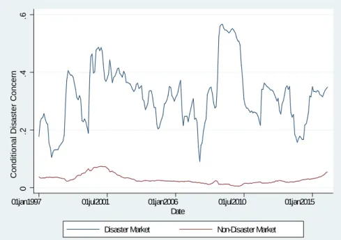
Figure 1 plots the market disaster concern along with the cross-sectional average stock disaster concern. The two variables tend to move in tandem with each other, and both exhibit wide ‡uctuations over time. In particular, there are two periods of substantial increase in the disaster concern of both the market index and individual stocks. The …rst one is the 1998–2002 period, corresponding to the Internet bubble and the subsequent bubble bursting, and the second one is the 2008–2011 period, corresponding to the recent …nancial crisis and the subsequent recession.
Figure 2 plots the cross-section average conditional disaster concern of stocks given the disaster and non-disaster market states, respectively. The average conditional disaster concern is always higher given disaster markets relative to non-disaster markets, meaning that investors are on average more concerned about future stock disasters if the market will have a disaster in the future than if not. Furthermore, while the average conditional disaster concern given non-disaster markets does not vary much over time, the average conditional disaster concern given disaster markets exhibits signi…cant time variations, with peaks around the crisis periods.
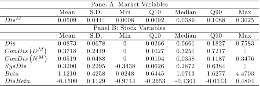
Table 1 reports summary statistics for the disaster concern variables. Panel A shows that the market disaster concern (DisM), estimated based on option prices of the S&P 500 index, has a mean value of 0.0509, indicating that investors expect a market-wide disaster to happen with a risk-neutral probability of 5% on average. The median ofDisM is 0.0389, and the standard deviation is 0.0444. The minimum and maximum are 0.0008 and 0.3025, respectively, meaning that the market disaster concern is considered close to zero during the safest time but as high as 30% during the riskiest time.
Panel B reports summary statistics for stock-level variables. For each of these variables, I …rst compute the average value for each stock over time, and then report the cross-sectional summary statistics of these stock averages. The cross-cross-sectional mean of the stock disaster concern (Dis) is 0.0873, indicating that an average …rm is expected to experience a disaster with a risk-neutral probability of around 9%. The median is 0.0661, and the standard deviation is 0.0678. The minimum and maximum are 0 and 0.7583, respectively, highlighting the wide cross-sectional variations in the disaster concern of di¤erent stocks.
The conditional disaster concern variables have very di¤erent statistics depending on the state of the market. Given disaster markets, the conditional disaster concern (ConDis DM )
has a mean value of 0.3718, implying that if the market will be in the disaster state, an average …rm is expected to experience a disaster with a risk-neutral probability of 37%. The median is 0.3251, and the standard deviation is 0.2419. The minimum and maximum are 0 and 1, respectively. This means that some …rms are considered to have a zero prob-ability of disaster even if the market itself will experience a disaster, whereas some other …rms are expected to have a disaster for sure if a market-wide occurs.
In comparison, given non-disaster markets, the conditional disaster concernConDis NM
has a much lower cross-sectional mean of 0.0519. This implies that …rms are considered much less likely to have a disaster if the market will not have a disaster than if it will. The median value is 0.0358. The standard deviation is 0.0488, also much lower than that ofConDis DM ;meaning that conditional on future non-disaster markets, …rms are con-sidered less heterogeneous in terms of how likely a disaster would happen. The minimum ofConDis NM is 0, and the maximum is 0.3476.
The systematic disaster concern (SysDis) has a mean of 0.3200, indicating that an average …rm is considered more likely to experience a disaster in disaster markets than in non-disaster markets by a risk-neutral probability of 32%. The standard deviation is 0.2295, which is mostly driven by the cross-sectional heterogeneity in ConDis DM :
Over 90% of all stocks have positiveSysDisestimates on average, as suggested by a 10th quantile of 0.0626. The cross-sectional minimum ofSysDisis a negative value of -0.3438, meaning that some …rms are considered more likely to experience a disaster if the market will perform normally relative to if the market will have a disaster. The cross-sectional maximum ofSysDisis 1, which can only happen when the conditional disaster concern is 1 given disaster markets and 0 given non-disaster markets.
Panel B of Table 1 also reports summary statistics for the CAPM beta (Beta) of the stocks. At the end of each month, I estimateBetafor each stock by regressing daily excess stock returns on daily excess market returns over the preceding twelve-month window. For consistency, I continue to use the S&P 500 as the market index for the estimation of Beta. Across my sample stocks, Beta has a mean of 1.1210, a median of 1.0713, and a standard deviation of 0.4258. All stocks have positive betas on average, with a
cross-sectional minimum of 0.0248 and a cross-cross-sectional maximum of 4.4703.
At the end of each month, I also estimate the market disaster concern beta (DisBeta) for each stock, which is obtained by regressing daily stock returns on daily estimates of DisM over the preceding twelve-month window. Intuitively, DisBeta measures the sensitivity of the stock return to the market disaster concern, which is similar to the approach commonly used in the literature to gauge the systematic disaster risk of individual stocks. Panel B of Table 1 shows that most stocks have negative DisBeta on average, suggesting that stocks tend to have lower returns as the market disaster concern rises. In fact, a more negative value of DisBeta indicates a larger decrease in the stock return when the market disaster concern rises, representing higher systematic disaster risk. The cross-sectional mean and median ofDisBetaare -0.1509 and -0.1301, respectively, and the cross-sectional standard deviation is 0.1129.
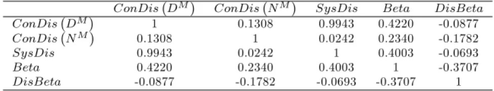
Table 2 reports the pairwise correlations across the stock-level variables. It shows that
ConDis DM andConDis NM have a mild positive correlation of 0.1308. Also,SysDis
has a very high correlation of 0.9943 with ConDis DM and only a weak correlation of 0.0242 withConDis NM :This suggests that the variations inSysDisare mostly driven byConDis DM :In addition,SysDisis positively correlated withBetawith a correlation coe¢ cient of 0.4003. Somewhat surprisingly, SysDis and DisBeta have a very small negative correlation of -0.0693. This suggests that these two measures are likely to capture di¤erent aspects of individual stocks’ exposure to systematic disaster risk. Furthermore,
DisBetais negatively correlated with Beta with a correlation coe¢ cient of -0.3707. The constrained regression estimation approach introduced in Section 3.2 implies that the market disaster concern is a factor driving the time variations in the disaster concern of individual stocks. It is then curious to ask what proportions of the time variations in individual stock disaster concern can be explained by variations in the market disaster concern. To answer this question, I compute the R-squared from the constrained linear regression (10) as
R2 = 1 V ar(")
V ar(Dis);
where V ar(Dis) is the variance of the disaster concern of a stock over the estimation window, and V ar(") is the variance of the regression residuals. Intuitively, R2 measures
the proportion of the total time variations in the stock disaster concern that is attributable to changes in the market disaster concern.
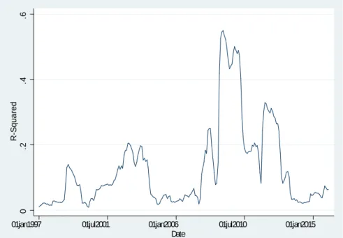
Figure 3 plots the cross-sectional average R-squared over time. The …gure shows that the average R-squared varies dramatically over the sample period. It tends to increase during crises. In particular, during the 2008–2009 …nancial crisis, the average R-squared rises sharply above 0.5, indicating that more than half of the time variations in individual stock disaster concern over this period is driven by changes in the market disaster concern.
4.3 Two Examples: Microsoft and Bank of America
To provide more intuitions about the systematic disaster concern of di¤erent stocks, I ex-amine Microsoft and BOA as two examples. We have seen in Figure 1 that there are two periods of substantial increases in the market disaster concern throughout my sample, with the 1998–2002 period driven by the Internet bubble and the 2008–2011 period correspond-ing to the …nancial crisis. Since Microsoft is a technology …rm and BOA is a …nancial …rm, one would wonder if these two …rms respond di¤erently over these two periods.
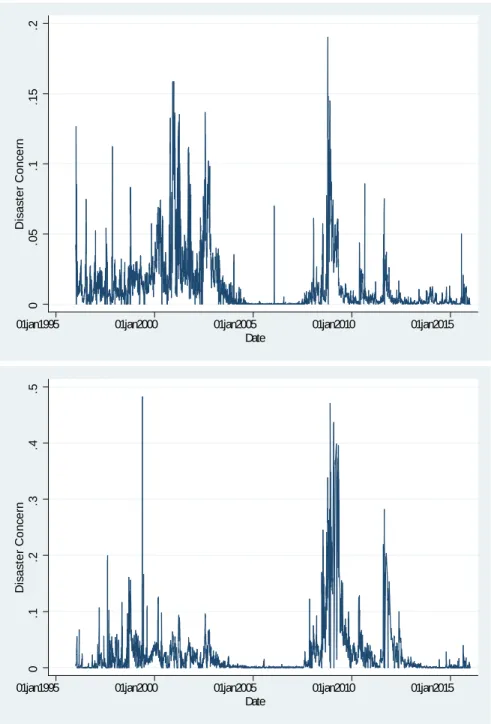
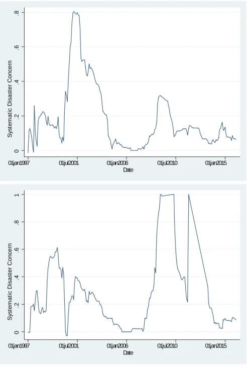
To address this question, I …rst plot the disaster concern of Microsoft and BOA over time in Figure 4. Both stocks exhibit dramatic increases in the disaster concern during both the 1998–2002 and the 2008–2011 periods, re‡ecting that the disaster concern of both stocks responds positively to increases in the market disaster concern. Interestingly, in the top …gure the increase in the disaster concern of Microsoft is more pronounced during the …rst period. In contrast, the bottom …gure shows that the increase in the disaster concern of BOA is more pronounced during the second period. This suggests that the disaster concern of Microsoft appears to be more sensitive to the increase in the market disaster concern driven by the Internet bubble, whereas the disaster concern of BOA appears to be more sensitive to the increase in the market disaster concern driven by the …nancial crisis. I further plot the systematic disaster concern of these two stocks over time in Figure 5, which directly measures the sensitivity of individual stock disaster concern to the market disaster concern. As expected, in the top …gure the systematic disaster concern of Microsoft rises sharply to around 0.8 during the Internet bubble, compared to a much milder rise during the …nancial crisis. In contrast, the bottom …gure shows that the systematic disaster concern of BOA shoots up to 1 during the …nancial crisis, much higher than its peak level
during the Internet bubble. These …ndings are consistent with intuitions and serve as supportive evidence for the validity of my estimation.
4.4 Condition Disaster Concern and Future Stock Disasters
The conditional disaster concern re‡ects investors’expectation on how likely a stock-level disaster is to happen in di¤erent market states. It is interesting to ask whether the esti-mated conditional disaster concern variables provide information on the future occurrence of stock disasters in the corresponding state of the market.
At any timet, two conditional disaster concern variables,ConDisit DM andConDisit NM ;
can be estimated for each stockicorresponding to future disaster and non-disaster markets, respectively. Eventually, only one of these two market states realizes, and the conditional disaster concern given the subsequently realized market state should be more relevant to the prediction of future stock disasters. Based on this idea, I denote byConDisit rMt+1 the conditional disaster concern of stocki estimated at the end of montht given the realized state of the market in month t+ 1;i.e.,
ConDisit rtM+1 = ConDis
i
t DM ; ifrMt+1 0:1
ConDisit NM ; ifrMt+1> 0:1 :
I further de…ne a dummy variable DisDti for a realized disaster of stock iin month t; i.e.,
DisDti= 1; ifr
i
t 0:25
0; ifrit> 0:25 :
If my conditional disaster concern estimates are informative,ConDisit rtM+1 should posi-tively predicts DisDti+1:
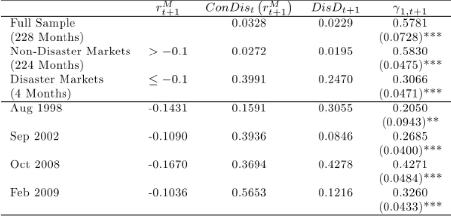
Table 3 comparesConDisit rtM+1 with DisDti+1:The average value ofConDisit rtM+1
across all stocks over the entire sample is 0.0328, meaning that on average investors ex-pect a stock-level disaster to occur with a risk-neutral probability of 3% conditional on the subsequently realized state of the market. The average value of DisDi
t+1 is 0.0229, indicating that the frequency of a realized stock disaster is about 2% in my sample. The table also reports results for subsamples with realized disaster and non-disaster markets separately. For the 224 months without market disasters (rMt+1> 0:1), the average value ofConDisit rtM+1 is 0.0272, and the average value ofDisDti+1is 0.0195. For the remaining
4 months with realized market disasters (rM
t+1 0:1), the average of ConDisit rMt+1 is 0.3391, and the average of DisDi
t+1 is 0.2470. This indicates that both the conditional disaster concern and the realized disaster frequency of stocks are higher given disaster markets relative to non-disaster markets. Notice that since ConDisit rMt+1 is de…ned un-der the risk-neutral measure and DisDit+1 re‡ects the frequency of stock disasters under the physical measure, the di¤erence in the average value between these two variables may result from both biased expectation and risk aversion of investors.
To see if stocks with higher ConDisit rMt+1 are more likely to experience disasters, for each montht; I run a cross-sectional regression of DisDit+1 onConDisit rtM+1 ;i.e.,
DisDit+1 = 0;t+1+ 1;t+1ConDist rtM+1 + t+1:
IfConDisi
t rtM+1 contains information on the realization of stock disasters, 1;t+1 should be positive.
The last column of Table 3 reports the time average of the estimated 1;t+1. For the entire sample, 1;t+1has a positive mean value of 0.5781, which is signi…cant at the 1% level based on the Newey-West standard error.2 This means that on average, ifConDisit rtM+1
increases from 0 to 1, the probability of a stock disaster increases by 58%. For the sub-samples with realized disaster and non-disaster markets, the average values of 1;t+1 are 0.3066 and 0.5830, respectively, both strongly signi…cant. This implies that increasing
ConDisit rMt+1 from 0 to 1 raises the probability of a stock disaster by 31% and 58% given realized disaster and non-disaster markets, respectively.
It is worth taking a closer look at each of the 4 months with realized market disasters. These 4 months are August 1998, September 2002, October 2008 and February 2009, with the monthly market return being -0.1431, -0.1090, -0.1670, and -0.1036, respectively. The lower panel of Table 3 shows that the estimated 1;t+1 is signi…cantly positive in each of these months, with values ranging from 0.2050 to 0.4271.
2
The Newey-West standard error is used to account for potential autocorrelation of the error term. Following Stock and Watson (2011) page 599, I choose the number of lags using the rule of thumb:
L= 0:75T1=3;
whereLis the number of lags andT is the number of observations in the time series. There are 228 months in my sample, which leads to the use of 5 lags.
Overall, these results show that my estimated conditional disaster concern variables indeed provide useful information on the future occurrence of stock disasters in the corre-sponding state of the market.
4.5 Systematic Disaster Concern and Expected Stock Returns
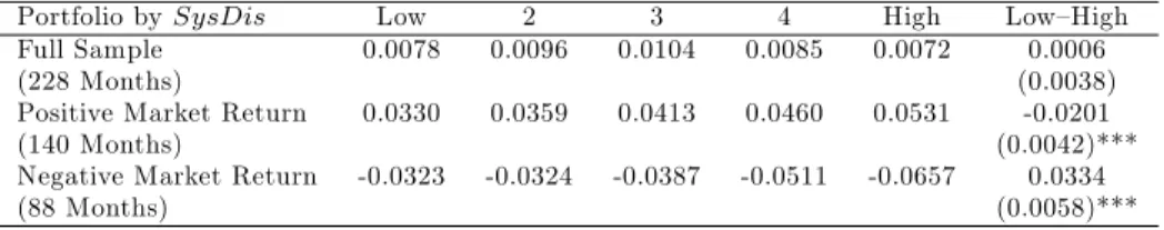
I now explore the relation between systematic disaster concern and the expected stock return. I start with a portfolio sorting approach. At the end of each month, I sort all stocks into …ve quintile portfolios by their systematic disaster concern estimates, and then calculate the equal-weighted return of each portfolio over the next month. Table 4 reports the average returns of the …veSysDis-sorted portfolios over time. From the lowest-SysDis
portfolio to the highest-SysDisportfolio, the average returns of the …ve portfolios over the entire sample are 0.0078, 0.0096, 0.0104, 0.0085 and 0.0072, respectively, which exhibit a hump shape. Portfolios with the lowest and highest systematic disaster concern tend to have lower returns on average than portfolios in the middle. The return di¤erence between the bottom and top portfolios is not signi…cantly di¤erent from zero.
To …nd out what drives the hump-shaped relation, I then calculate the average returns of the …veSysDis-sorted portfolios over months with positive and negative market returns separately. For the 140 months with positive market returns, the average returns of the …ve portfolios from the lowestSysDisto the highestSysDisare 0.0330, 0.0359, 0.0413, 0.0460, and 0.0531, respectively, which are monotonically increasing. The average return di¤erence between the bottom and the top portfolios is -0.0201, and this di¤erence is signi…cant at the 1% level. This suggests that stocks with high systematic disaster concern outperform stocks with low systematic disaster concern on average when the market overall performs well. In particular, going long in stocks with the highestSysDisand shorting stocks with the lowestSysDisresults in an average monthly return of 2.01% conditional on the market delivering positive returns.
I then repeat the analysis for the 88 months with negative market returns. The average returns of the …ve portfolios from the lowest SysDis to the highest SysDis are -0.0323, -0.0324, -0.0387, -0.0511, and -0.0657, respectively, which are monotonically decreasing. The average return di¤erence between the bottom and the top portfolios is 0.0334, also signi…cant at the 1% level. This shows that stocks with high systematic disaster concern
underperform stocks with low systematic disaster concern on average when the market overall performs poorly. In particular, going long in stocks with the lowest SysDis and shorting stocks with the highest SysDis results in an average monthly return of 3.34% conditional on the market return being negative.
The opposite relations between the systematic disaster concern and the expected portfo-lio return in good and bad markets are intuitive. The systematic disaster concern describes investors’expectations on the incremental likelihood of future stock disasters if there will be a market-wide disaster relative to if there will not. It has been shown in Section 4.4 that these expectations are indeed informative on the future occurrence of stock disasters in di¤erent states of the market. Given this, if a market-wide disaster happens in the future, one would expect stocks with high systematic disaster concern to be more heavily a¤ected and hence deliver lower returns than other stocks. In addition, given the continuous na-ture of equity returns, negative market returns above the disaster threshold, despite being de…ned as in the non-disaster state, also represent poor performance of the market. As a result, stocks with high systematic disaster concern may underperform in this situation as well. In contrast, when the market performs well, stocks with high systematic disaster concern should outperform other stocks. Otherwise, they would be dominated by stocks with low systematic disaster concern in all market states, and thus no investors would be willing to hold them. This explains the positive relation between systematic disaster concern and the expected portfolio return conditional on the future market return being positive. Overall, the opposite patterns in good and bad markets together give rise to the hump-shaped relation between systematic disaster concern and expected portfolio returns in the full sample.
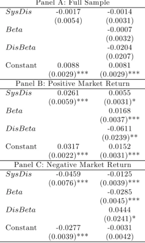
The analysis so far is at the portfolio level. To further examine the relation between systematic disaster concern and the expected stock return in di¤erent market states, I use a regression approach at the stock level. In each month, I cross-sectionally regress the monthly stock return on the systematic disaster concern estimated as of the end of the previous month, controlling for lagged values of the CAPM beta (Beta) and the market disaster concern beta (DisBeta), i.e.,
The reason for includingBeta in the regression is because it is positively correlated with
SysDis:Stocks with largeBetaare cyclical in the sense that they tend to outperform other stocks in good markets and underperform other stocks in bad markets. I thus wonder if the relation between the systematic disaster concern and the expected stock return in di¤erent market states is driven byBeta. I also control forDisBetain the regression to disentangle the e¤ects ofSysDisand DisBetaon the expected stock return.
Table 5 shows the average values of the regression coe¢ cients over time. I start by running the regression without controlling for Beta and DisBeta: Over the full sample, the average slope coe¢ cient on SysDis is not signi…cantly di¤erent from zero, which is expected given the hump-shaped relation found with the portfolio sorting approach. I then split the full sample into subsamples with positive and negative monthly market returns. For the months with positive market returns, the average coe¢ cient on SysDis
is signi…cant positive at the 1% level, implying that stocks with higher systematic disaster concern tend to deliver higher returns in good markets. On the other hand, for the months with negative market returns, the average coe¢ cient onSysDisis negative and signi…cant at the 1% level, implying that stocks with higher systematic disaster concern tend to deliver lower returns in bad markets. These …nding are consistent with the results from portfolios sorting
I then include Beta and DisBeta in the regression. For the full sample, including the controls does not change the result much. The average coe¢ cient on SysDisremains insigni…cant. In fact, neither Beta nor DisBeta seems to have a signi…cant e¤ect on the expected stock return over the entire sample. For the months with positive market returns,
Beta has a positive coe¢ cient and DisBetahas a negative coe¢ cient, and both variables are statistically signi…cant. This means that stocks with higher Beta and lower DisBeta
tend to deliver higher returns if the market performs well. With these variables being controlled for,SysDisis still positive and signi…cant at the 10% level. This indicates that the positive relation between SysDis and the expected stock return in good markets is not fully driven by Beta and DisBeta: When I focus on months with negative market returns, I now …nd a negative coe¢ cient on Beta and a positive coe¢ cient on DisBeta;
meaning that stocks with lower Beta and higher DisBeta tend to perform better in bad markets. Interestingly, the coe¢ cient on SysDis remain negative and signi…cant at the
1% level. This shows that the negative relation between SysDis and the expected stock return remains strong even whenBeta and DisBetaare controlled for.
Overall, my results show that the relation between systematic disaster concern and the expected stock return depends on the market state. Higher systematic disaster concern predicts higher stock returns in good markets and lower stock returns in bad markets. These e¤ects are not driven by the CAPM beta or the market disaster concern beta.
4.6 A Trading Strategy
Section 4.5 shows that stocks with the lowest and the highest systematic disaster concern have lower expected returns than stocks in the middle. This allows me to construct a trading strategy by going long in stocks with middle levels of systematic disaster concern and shorting a combination of stocks with the lowest and the highest systematic disaster concern.
Let rpj
t+1 represent the equal-weighted return of the jth quintile portfolio sorted by
SysDist over montht+ 1;wherej= 1;2; : : :5:The trading return from going long in the
middle quintile and shorting a combination of x in the bottom quintile and 1 x in the top quintile is rtT rade+1 =rp3 t+1 xr p1 t+1 (1 x)r p5 t+1; (11)
where x takes values from 0 to 1.3 In particular, x = 0corresponds to going long in the mid-SysDisportfolio and shorting the highest-SysDisportfolio, andx= 1corresponds to going long in the mid-SysDisportfolio and shorting the lowest-SysDisportfolio. A larger
x represents shorting a larger proportion of stocks with the lowest systematic disaster concern.
Table 6 reports the average returns from the trading strategy withxvarying from 0 to 1. The average monthly trading return is positive for all values of x: It slowly decreases from 0.32% whenx= 0 to 0.26% whenx= 1;which is a result of the fact that the
lowest-SysDis portfolio has a slightly higher average return than the highest-SysDis portfolio during the sample period. Statistically,x = 0:7 gives rise to the most signi…cant average
3
The trading strategy proposed here is a long-short strategy that requires zero net investment. The trading return (11) represents the pro…t earned for each one dollar engaged in the long-short strategy. One can easily scale up or down the trading pro…t while maintaining zero net investment.
trading return of 0.28%, corresponding to a long position in the mid-SysDisportfolio and a short position consisting of 70% in the lowest-SysDis portfolio and 30% in the
highest-SysDisportfolio. The statistical signi…cance results from reduced trading volatility from shorting a non-zero proportion of both the lowest-SysDisand the highest-SysDisstocks, since these two groups of stocks tend to have o¤setting returns.
To understand the source of the positive average trading returns, I calculate the abnor-mal returns (i.e., risk-adjusted alphas) with respect to a number of popular factor models. I start with the CAPM model, in which the market factor is the only source of systematic risk. The CAPM alpha ranges from 0.65% when x = 0 to 0.15% when x = 1; and it is signi…cantly positive at the 5% level for values ofxbetween 0 and 0.7. This indicates that the positive average trading returns are not attributable to the exposure of my trading strategy to the market risk. I next estimate the alpha using the Fama and French (1993) three factors (market, size, and value) plus a fourth momentum factor (Carhart (1997)). The four-factor alpha ranges from 0.41% when x = 0 to 0.25% when x = 1: Indeed, for almost all values ofx;the four-factor alpha is weakly higher than the corresponding average trading return and statistically signi…cant. Again, my trading strategy generates positive abnormal returns that cannot be explained by the market, size, value, and momentum factors. Finally, I estimate the risk-adjusted alpha using the Fama and French (2016) …ve factors (market, size, value, pro…tability, and investment) plus the momentum factor. Now the abnormal return disappears for all values ofx:This suggests that the positive average trading returns are mostly driven by the pro…tability and investment factors.4
Finally, Table 7 reports the slope coe¢ cients and the adjusted R-squared from re-gressing the trading returns on the Fama-French …ve factors and the momentum factor for di¤erent values of x: Each factor has a signi…cant coe¢ cient for at least some values of x: The adjusted R-squared ranges from 0.6991 when x = 0 to 0.3309 when x = 1:
Hence, the six factors together explain 33%–70% of the variations in the returns from the
SysDis-based trading strategy. 4
Including the Pástor and Stambaugh (2003) liquidity factor does not change the results. I thus omit it for brevity.
4.7 Systematic Disaster Concern and Firm Characteristics
This section examines the relation between systematic disaster concern and various stock and …rm characteristics. I focus on the following characteristics:
CAPM beta (Beta): the sensitivity of the stock return to the market return (proxied by the S&P 500 return);
Market disaster concern beta (DisBeta): the sensitivity of the stock return to the market disaster concern (DisM);
Idiosyncratic volatility (Idio): the annualized standard deviation of the residuals from the CAPM regression;
Illiquidity (Illiq): the average of daily ratios of the absolute stock return to the dollar trading volume, scaled by the cross-sectional mean (following Amihud (2002)); Firm size (Size): the log market capitalization;
Book-to-market ratio (B2M): the ratio of the book value of equity to the market value of equity;
Return on equity (ROE): the ratio of income before extraordinary items to the book value of equity;
Investment (Inv): the proportional quarterly change in total assets; Leverage (Lever): the ratio of total liabilities to total assets.
At the end of each month, I estimateBeta; DisBeta; IdioandIlliqusing stock returns and other information at the daily frequency from the most recent twelve-month window. This is consistent with the window period used to estimate the systematic disaster concern
SysDis. For Size; B2M; ROE; Inv and Lever; I use the most recent values of these variables available as of the end of each month. To examine the relation between system-atic disaster concern and the characteristics, in each month I again sort stocks into …ve quintile portfolios based on SysDis, and I compute the equal-weighted average value of
each characteristic for the …ve portfolios. I use values of SysDis and the characteristics in the same month instead of looking at the lead-lag relation, since the focus here is not about prediction.
Table 8 reports the time averages of SysDis and the characteristics for the SysDis -sorted portfolios. The average values ofSysDisfor the …ve portfolios are -0.0103, 0.0917, 0.2121, 0.4016 and 0.7433, respectively. The average portfolio characteristics exhibit some nonlinearity with respect toSysDis, and a closer look reveals that the nonlinearity comes solely from the lowest-SysDisportfolio. Ignoring the lowest-SysDisportfolio, I …nd that portfolios with higher SysDis are associated with larger CAPM betas, more negative market disaster concern betas, higher idiosyncratic volatility and illiquidity, smaller market capitalization, lower returns on equity and leverage, and higher book-to-market ratios and investment. On the other hand, the lowest-SysDis portfolio has the highest level of illiquidity of all …ve portfolios, and it also tends to contain stocks with small market capitalization and below-average CAPM betas. Such stocks may be less likely to draw attention from investors and hence less actively traded. This in turn may cause the stock disaster concern to be less sensitive to the market disaster concern, thus giving rise to very low levels of systematic disaster concern.
5
Conclusion
The existing literature on the option-implied disaster concern is restricted to the aggregate market. This paper extends the literature by studying individual assets’disaster concern and its systematic variations with the market. I propose new measures of the conditional and systematic disaster concern of an asset with respect to the market index, which can be estimated based on the comovement of the option-implied disaster concern between the asset and the market index. These measures have intuitive interpretations in terms of the risk-neutral conditional disaster probabilities, re‡ecting investors’expectations on the asset disaster risk given di¤erent future states of the market. Using the S&P 500 index as the proxy for the market index, I empirically estimate the conditional and systematic disaster concern measures for a large set of common stocks. I show that the estimated conditional and systematic disaster concern variables vary widely both in the time series
and in the cross section and that they strongly predict stock-level disasters and stock returns in di¤erent market states. These …ndings indicate that the comovement of option prices between stocks and the market index contains forward-looking information on their joint tail distributions.
The idea of using the covariations in the option prices of di¤erent securities to infer their joint return behavior extends far beyond the study of disaster risk. By de…ning richer state spaces, one could potentially estimate the entire risk-neutral joint return distrib-utions of di¤erent securities from option prices. In addition, the constrained regression approach motivated by the total probability formula is nonparametric and does not rely on an assumed functional form of the generating process of asset returns. Hence, it may help uncover potential nonlinearity in the structure of asset returns with respect to systematic factors. All of these could have important implications on theoretical and empirical work in asset pricing, which I leave for future research.
Appendix: Estimating European Option Prices
As discussed in Section 3.1, in order to estimate the disaster concern of an asset, one needs European put option prices for some speci…c time to maturity and strike prices around the disaster threshold, which are usually not directly observed in the market. To obtain these option prices, I adopt the following approach from the literature (e.g., Shimko (1993), Malz (1997), and Figlewski (2010)). On any given date, I start with the implied volatilities provided in OptionMetrics of all traded options written on the asset of interest, and …t the implied volatility surface across di¤erent strike prices and maturities. Then, I plug the …tted implied volatilities at the required maturity and strike prices into the BS pricing formula to estimate the corresponding European option prices.
I …t the implied volatility surface by kernel smoothing, following the procedure used by OptionMetrics. For each date, I index all traded option contracts written on the asset by h = 1;2; : : : ; H: For each option contract h, let h represent the implied volatility, and let Vh be the option vega (which measures the sensitivity of the option price to the volatility). Denote by mnh = Xh=St the moneyness of the option, by mth the time to
put options. Then, for any arbitrary moneyness mn (within the range of moneyness for traded options), time to maturitymt (within the range of maturity for traded options), and call-put indicator cp (cp = 1 for all my analyses since I use put option prices for disaster concern estimation), the …tted volatility can be computed as
^ (mn ; mt ; cp ) = PH h=1Vh h mn mnh; mt mth; cp cph PH h=1Vh (mn mnh; mt mth; cp cph) ; (12) where the kernel function is given by
(x; y; z) = p1 2 exp x2 2c1 y2 2c2 z2 2c3 :
I naively choose c1 = c2 =c3 = 0:001: I check to make sure that these parameter values yield reasonable …tting.
The idea of the kernel smoothing procedure is intuitive. For any (mn ; mt ; cp ), I estimate the associated implied volatility as the weighted average of the implied volatilities of all traded options, where those with moneyness, time to maturity, and call-put indicator close to(mn ; mt ; cp )are assigned higher weights than those far away. In addition, since I eventually need to compute the European option prices from the …tted implied volatilities, I also assign higher weights to traded options whose prices have higher sensitivity to the volatility (higher vega).
It is worth mentioning that the kernel smoothing formula (12) applies only for values of mn and mt within the observed ranges of the corresponding parameters for traded options. In order to estimate the disaster concern, I need European put option prices (and hence the volatilities) around the disaster thresholds, and thus mn may lie below the observed moneyness range of traded options. In this case, I assume that the implied volatility outside the observed range is ‡at and hence setmn equal to the lowest observed moneyness of traded options.
References
[1] Amihud, Yakov, 2002. Illiquidity and stock returns: cross-section and time-series ef-fects. Journal of …nancial markets 5, 31–56.